3D Tiled Code Generation for Nussinov’s Algorithm

Abstract

Current state-of-the-art parallel codes used to calculate the maximum number of pairs for a given RNA sequence by means of Nussinov’s algorithm do not allow for achieving speedup close up to the number of the processors used for execution of those codes on multi-core computers. This is due to the fact that known codes do not make full use of and derive benefit from cache memory of such computers. There is a need to develop new approaches allowing for increasing cache exploitation in multi-core computers. One of such possibilities is increasing the dimension of tiles in generated target tiled code and assuring a similar size of generated tiles. The article presents an approach allowing us to produce 3D parallel code with tiling calculating Nussinov’s RNA folding, i.e., code with the maximal tile dimension possible for the loop nest, executing Nussinov’s algorithm. The approach guarantees that generated tiles are of a similar size. The code generated with the presented approach is characterized by increased code locality and outperforms all closely related ones examined by us. This allows us to considerably reduce execution time required for computing the maximum number of pairs of any nested structure for larger RNA sequences by means of Nussinov’s algorithm.

1. Introduction

The goal of this article is to show a way to create 3D parallel tiled code from serial dynamic programming code executing Nussinov’s RNA folding algorithm. There exist different serial implementations of that algorithm, but the main drawbacks of those programs are poor performance and cache efficiency for a large problem size. Parallelization and loop tiling transformations are used to enhance serial code performance. Loop tiling is often applied to optimize both serial and parallel programs. It increases parallel code granularity and data locality for multi-core architectures. Our goal is to generate code enumerating tiles whose dimension is maximal because the greater the tile dimension is, the more tiled code locality is reached. On the other hand, we aim to generate tiles of a similar size because such tiles allow us to better balance thread load, which improves parallel code performance. The maximal tile dimension of a loop nest is defined with the number of loops in that nest. Nussinov’s algorithm is implemented with a nest including three loops, so for that nest, the maximal tile dimensions are 3D. There are known codes implementing 2D tiling for Nussinov’s algorithm, for example [1,2]. The articles [3,4] introduce 3D tiling for Nussinov’s algorithm, but generated tiles are of different sizes and some tiles are parametric, i.e., their size is unlimited. This makes it very difficult to balance thread load and as a consequence reaching the maximal performance of those parallel tiled codes is impossible. In this article, we present a method of creating the 3D parallel tiled program with tiles of a similar bounded size, implementing Nussinov’s algorithm and showing the advantages of that code. The major contributions of the article are the following.

• Proposition of a modification of Nussinov’s algorithm to a form allowing us to produce 3D parallel tiled code with tiles of a similar bounded size.
• Presentation of a way to produce 3D parallel tiled code implementing Nussinov’s algorithm.
• Demonstration of the generated 3D parallel tiled code performance on different platforms and the comparison of its performance with that of known implementations of Nussinov’s algorithm.

The rest of this article is organized as follows. Section 2 introduces background and notations. Section 3 shows a method of generation of 3D parallel tiled code. Section 4 presents related work. Section 5 discusses experimental results. Section 6 includes conclusions.

2. Background

The algorithm by Nussinov et al. [5] aims at computing the maximal number of base pairs for any nested structure or a given RNA sequence. For this purpose, dynamic programming is applied. Recursions are used to fill table S, where an entry $S(i,j)$ holds the maximal number of base pairs for the subsequence from position i to j. The entry $S(0,n-1)$ (adapted to an implementation in the C language) provides the overall maximal number of base pairs for the whole sequence of length n. Let S be an $n\times n$ Nussinov matrix and $sigma(i,j)$ be a function which returns 1 if $(x_i,x_j)$ match and $i<j$, or 0 otherwise; then, the following recursion $S(i,j)$ (the maximum number of base-pair matches of $x_i,\dots ,x_j$) is defined over the region $0\le i<j<n,i\le k<j$ as follows [5].

$$S(i,j)=\underset{0\le i<j<n}{max}\{\begin{array}{c}S(i,j-1)\hfill \\ \underset{i\le k<j}{max}\left(S\right(i,k-1)+S(k+1,j-1)+\sigma (i,j\left)\right)\hfill \end{array}$$

(1)

There are different semantically identical codes implementing Nussinov’s recurrence. In this article, we use the popular C code introduced in article [1] and presented in Listing 1. Despite the fact that the code does not use the same statements as those in the original Nussinov recurrence, it carries out the same calculations as the original recurrence; therefore, it produces the same output that the original recurrence does. The reason for the usage of that code is its property relying on decrementing the value of index i; this allows us to build a calculation model used for deriving the proposed approach for the generation of 3D tiles.

Listing 1. Nussinov’s loop nest.

1	for ( i = n−1; i >= 0; i −−) {
2	for (j = i + 1; j < n; j ++) {
3	for (k = i; k < j ; k ++) {
4	S[ i ][ j ]=max(S[ i ][ k ] + S[k + 1][j], S[ i ][ j ]); // s1
5	}
6	S[ i ][ j ]=max(S[ i ][ j ], S[i + 1][j − 1] + sigma( i , j )); // s2
7	}
8	}

Listing 1. Nussinov’s loop nest.

1	for ( i = n−1; i >= 0; i −−) {
2	for (j = i + 1; j < n; j ++) {
3	for (k = i; k < j ; k ++) {
4	S[ i ][ j ]=max(S[ i ][ k ] + S[k + 1][j], S[ i ][ j ]); // s1
5	}
6	S[ i ][ j ]=max(S[ i ][ j ], S[i + 1][j − 1] + sigma( i , j )); // s2
7	}
8	}

Program code can expose dependences among instances of loop statements. A dependence takes place when two statement instances access the same memory cell and at least one of these accesses is write. Each dependence available in an original code should be respected in the code generated from the original one.

To transform the code implementing original Nussinov’s algorithm, we use the iscc calculator [6], which implements operations on polyhedral sets and relations according to the article [7].

To transform the code implementing original Nussinov’s algorithm, we form a set of the form $\left\{\right[\mathit{input\; list}]\mid \mathit{formula}\}$, where input list is the list of expressions used to describe a set tuple; formula describes the constraints imposed upon the set tuple. It is a Presburger formula including constraints represented by affine expressions connected with logical and existential operators.

3. Materials and Methods, 3D Tiled Code Generation

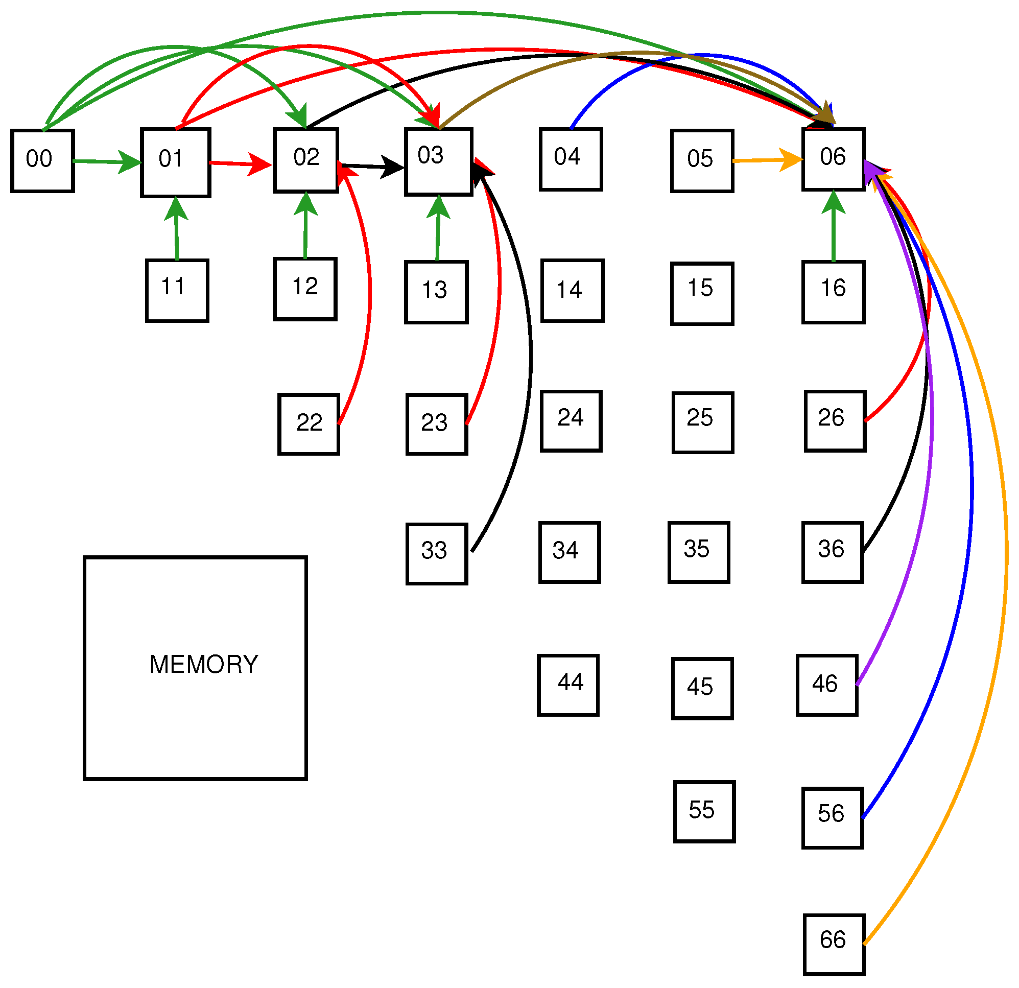
To implement the calculations represented with Listing 1, we use a calculation model based on a network of computational cells suggested by Figure 1 for $n=7$, that is, a triangle of cells. Each cell runs instances of statement S1 and statement S2. Cells use shared memory for reading and writing results produced with them. So, results calculated by cells are held in shared memory. At a particular time unit, cell $(i,j)$ updates the value of $S(i,j)$ running an instance of statement S1 when the values produced with instances of S1 by means of cells $(i,k)$ and $(k+1,j)$, which we call the horizontal and vertical mates of cell $(i,j)$, respectively, are ready (already updated). In Figure 1, the mates of cells 01, 02, 03, and 06 are connected with those cells with the arrows in the same color. The rest of the arrows connecting a cell with its mates are skipped in order to not clutter the drawing.

Taking into account that before calculation, i.e., in time unit 0, for a given $i,i=1,2,\dots ,n-1$, $S(i,i)=0$ and supposing that each cell requires one time unit to complete the execution of an instance of statement S1, from Figure 1, we conclude that for a cell ($i,j)$ and a given k, the time unit of completing the calculation of a horizontal mate is the following $t1=k-i$, whereas the time unit of completing the calculation of a vertical mate is as follows: $t2=j-k-1$. For example, for cell 01 its mates 00 and 11 are ready at time 0 because for cell 01, $k=0$.

As far as statement S2 is concerned, it is to be executed at the time unit when the value of $S(i,j)$ produced with statement S1 by means of loop k has already been completed (completing the execution of loop k for given values of i and j).

From Figure 1, it is clear that for cell ($i,j)$, the time unit of completing the calculation of S1 with loop k is equal to $j-i$, for example, for cell 01 that time unit is 1, for cell 02 that time unit is 2, and so on.

To guarantee that statement S2 is executed at the time unit when loop k completes the calculation of S1, but after statement S1, we introduce the second time unit dimension whose value is 0 for statement S1 and 1 for statement S2, i.e., the time of completing S1 for cell 01 is (1,0), whereas the time of completing S2 for cell 01 is (1,1).

Table 1. Time units $t1,t2$ and the time units of completing S1, S2 for cells 01 to 06; $i\le k<j$.

Cell	k/Horizontal Mate/ $\mathit{t}1=\mathit{k}-\mathit{i}$	k/Vertical Mate/ $\mathit{t}2=\mathit{j}-\mathit{k}-1$	$\mathit{j}-\mathit{i}$	Time of S1	Time of S2
01	0/00/0	0/11/0	1	1, 0	1, 1
02	0/00/0 1/01/1	0/12/1 1/22/0	2	2, 0 2, 0	2, 1 2, 1
03	0/00/0 1/01/1 2/02/2	0/13/2 1/23/1 2/33/0	3	3, 0 2, 0 3, 0	3, 1 - 3, 1
04	0/00/0 1/01/1 2/02/2 3/03/3	0/14/3 1/24/2 2/34/1 3/44/0	4	4, 0 3, 0 3, 0 4, 0	4, 1 - - 4, 1
05	0/00/0 1/01/1 2/02/2 3/03/3 4/04/4	0/15/4 1/25/3 2/35/2 3/45/1 4/55/0	5	5, 0 4, 0 3, 0 4, 0 5, 0	5, 1 - - - 5, 1
06	0/00/0 1/01/1 2/02/2 3/03/3 4/04/4 5/05/5	0/16/5 1/26/4 2/36/3 3/46/2 4/56/1 5/66/0	6	6, 0 5, 0 4, 0 4, 0 5, 0 6, 0	6, 1 - - - - 6, 1

presents time units $t1$, $t2$ of completing the calculations of $S1(i,k)$ with statement S1 (a horizontal mate) and $S1(k+1,j)$ (a vertical mate) with statement S1 as well as the time units of completing the execution of statements S1 and S2 for cells 01 to 06. The time of the execution of statement $S1$ for given $i,j$ and k is calculated as $max(t1,t2)+1$, where $t1$ and $t2$ state for the completing time of the horizontal and vertical mates, respectively, i.e., next time after all the operands of statement $S1$ are ready. It is worth noting that statement $S2$ is executed only when all the iterations of loop k are already finished.

It is worth mentioning that at the same time unit, a cell can combine two or more pairs of values produced with mates for statement S1. For example, at time unit (2,0), cell 02 updates two times; at that time unit, it combines values generated with mates 00 and 12 as well as 01 and 22 because at time unit (2,0) all those mates complete their updating. In such a case, output dependences arise, which we will respect due to serial updates performed with the corresponding cell as described below in this section.

Table 2. Time units of the completion of all cells—the completion of S2.

Cell	Time Unit of Completing Cell $(\mathit{i},\mathit{j})$-Completing S2
01, 12, 23, 34, 45, 56	1, 1
02, 13, 24, 35, 46	2, 1
03, 14, 25, 36	3, 1
04, 15, 26	4, 1
05, 16	5, 1
06	6, 1

presents the time units of the completion of all cells shown in Figure 1—the time units of the completion of statement S2.

To generate code, we form the following set $CODE$ whose constraints take into account the consideration mentioned above.

$$\begin{array}{cc}\hfill CODE& :=\left[n\right]\to \left\{\right[t,i,j,k,s]\mid \exists t1,t2s.t.(\hfill \\ \hfill & 0\le i\le k<j<n\&t1=k-i\&t2=j-k-1\hfill \\ \hfill & \&t=max(t1,t2)+1\&(s=1\&t=j-i\vee s=0\&t\le j-i)\left)\right\}.\hfill \end{array}$$

In the set above, $\left[n\right]$ means that n is the parameter; $[t,i,j,k,s]$ is the set tuple where variable $t=max(t1,t2)+1$ defines a time unit when cell $(i,j)$ completing the execution of all instances of statement S1 using the values produced with cells $(i,k)$ and $(k+1,j)$, the value 0 of variable s ($s=0$) means that statement S1 should be executed, whereas the value 1 of variable s ($s=1$) means that statement S2 should be executed; variables $t1=k-i$ and $t2=j-k-1$ hold the time units of completing the calculations of horizontal and vertical mates, respectively; $0\le i\le k<j<n$ is the constraint of Nussinov’s recursion; the constraint $s=1\&t=j-i$ means that statement S2 $(s=1)$ is to be executed when $t=j-i$ whereas the constraint $s=0\&t\le j-i$ defines the condition when statement $S1(s=0)$ should be executed; & and ∨ denote the operators AND and OR, respectively.

Set $CODE$ allows us to generate target code that executes statement instances in the lexicographic order of vector ${(t,i,j,k,s)}^T$, i.e., the outermost loop is to enumerate the values of variable t; the next two loops are to enumerate the values of variables i and j. Because iterator k is dependent from variables $t,i$ and j, a code generator will skip a loop for enumerating k. The value of variable s points out what statement (S1 or S2) is to be executed.

Applying the iscc codegen operator [7] to $CODE$ set, we acquire the pseudo-code shown in Listing 2. It is worth noting that the value of variable s (0 or 1) implements also two-dimensional time units presented in Table 1 and Table 2. Because the code generator produces code that enumerates statement instances in lexicographic order, in the generated code, at the same time the unit defined with iterator $c0$ statement S2 is executed after statement S1.

Listing 2. Pseudo-code implementing tranformed Nussinov’s algorithm.

1	for (int c0 = 1; c0 < n; c0 += 1)
2	for (int c1 = 0; c1 < n − c0; c1 += 1)
3	for (int c2 = c0 + c1; c2 < min(n, 2 ∗ c0 + c1); c2 += 1)         {
4	if (2 ∗ c0 + c1 >= c2 + 2) {
5	(c0, c1, c2, −c0 + c2, 0);  //pseudo-statement
6	if (c2 == c0 + c1)
7	(c0, c1, c0 + c1, c1, 1);  //pseudo-statement
8	}
9	(c0, c1, c2, c0 + c1 − 1, 0);  //pseudo-statement
10	if (c2 == c0 + c1)
11	(c0, c1, c0 + c1, c0 + c1 − 1, 1); //pseudo-statement
12	}

Listing 2. Pseudo-code implementing tranformed Nussinov’s algorithm.

1	for (int c0 = 1; c0 < n; c0 += 1)
2	for (int c1 = 0; c1 < n − c0; c1 += 1)
3	for (int c2 = c0 + c1; c2 < min(n, 2 ∗ c0 + c1); c2 += 1)         {
4	if (2 ∗ c0 + c1 >= c2 + 2) {
5	(c0, c1, c2, −c0 + c2, 0);  //pseudo-statement
6	if (c2 == c0 + c1)
7	(c0, c1, c0 + c1, c1, 1);  //pseudo-statement
8	}
9	(c0, c1, c2, c0 + c1 − 1, 0);  //pseudo-statement
10	if (c2 == c0 + c1)
11	(c0, c1, c0 + c1, c0 + c1 − 1, 1); //pseudo-statement
12	}

We transform that pseudo-code to C code, taking into account that in the pseudo-code c0 and c1 correspond to t and i, respectively, in the tuple of set $CODE$; the third expression in each pseudo-statement relates to j, whereas the fourth one corresponds to k in the tuple of set $CODE$; the fifth element in each pseudo-statement defines the statement: 0 denotes statement S1 whereas 1 denotes statement S2. In the pseudo-code above, depending of the value of the fifth element of the corresponding pseudo-statement, we replace each pseudo-statement with the statement

S[i][j] = max(S[i][k] + S[k+1][j], S[i][j]); // S1

or the statement

S[i][j] = max(S[i][j], S[i+1][j−1] + sigma(i, j)); // S2

(S1 and S2 are the statements of the code in Listing 1) replacing variables $i,j$, and k with the second, third, and fourth expressions of the corresponding pseudo-statement and insert the definitions of the functions used in generated C code. The implementation of function $sigma$ is presented at: https://github.com/piotrbla/nuss3d (last accessed on 7 June 2022).

The target C code is presented in Listing 3.

Listing 3. Transformed Nussinov loop nest.

1	#define min(x,y)  ((x) < (y) ? (x) : (y))
2	#define max(x,y)  ((x) > (y) ? (x) : (y))
3	#define floord(n,d) (((n) < 0) ? −((−(n)+(d)−1)/(d)) : (n)/(d))
4	int sigma(int, int);
5
6	for (int c0 = 1; c0 < n; c0 += 1){
7	for (int c1 = 0; c1 < n − c0; c1 += 1){
8	for (int c2 = c0 + c1; c2 < min(n, 2 ∗ c0 + c1); c2 += 1)         {
9	if (2 ∗ c0 + c1 >= c2 + 2){
10	S[c1][c2] = max(S[c1][−c0 + c2] + S[−c0 + c2+1][c2],           S[c1][c2]); // s1
11	if (c2 == c0 + c1)
12	{
13	S[c1][c2] = max(S[c1][c2], S[c1+1][c2−1] + sigma(c1          , c2)); // s2
14	}
15	}
16	S[c1][c2] = max(S[c1][c0 + c1 − 1] + S[c0 + c1][c2], S          [c1][c2]); // s1
17	if (c2 == c0 + c1){
18	S[c1][c2] = max(S[c1][c2], S[c1+1][c2−1] + sigma(c1,           c2)); // s2
19	}
20	}
21	}
22	}

Listing 3. Transformed Nussinov loop nest.

1	#define min(x,y)  ((x) < (y) ? (x) : (y))
2	#define max(x,y)  ((x) > (y) ? (x) : (y))
3	#define floord(n,d) (((n) < 0) ? −((−(n)+(d)−1)/(d)) : (n)/(d))
4	int sigma(int, int);
5
6	for (int c0 = 1; c0 < n; c0 += 1){
7	for (int c1 = 0; c1 < n − c0; c1 += 1){
8	for (int c2 = c0 + c1; c2 < min(n, 2 ∗ c0 + c1); c2 += 1)         {
9	if (2 ∗ c0 + c1 >= c2 + 2){
10	S[c1][c2] = max(S[c1][−c0 + c2] + S[−c0 + c2+1][c2],           S[c1][c2]); // s1
11	if (c2 == c0 + c1)
12	{
13	S[c1][c2] = max(S[c1][c2], S[c1+1][c2−1] + sigma(c1          , c2)); // s2
14	}
15	}
16	S[c1][c2] = max(S[c1][c0 + c1 − 1] + S[c0 + c1][c2], S          [c1][c2]); // s1
17	if (c2 == c0 + c1){
18	S[c1][c2] = max(S[c1][c2], S[c1+1][c2−1] + sigma(c1,           c2)); // s2
19	}
20	}
21	}
22	}

The transformed Nussinov’s code is within re-ordered transformations. It runs the same calculations as those performed with Nussinov’s algorithm whose code is presented in Listing 1; but in a different order. A re-ordered transformation of an algorithm is legal if it runs the same calculations as those ran with the original one and honors all the dependences of that algorithm. The transformed Nussinov’s code is legal because (i) it runs the same calculations as those ran with the original one and (ii) honors all the dependences available of the original Nussinov’s algorithm as we explain below. There exists two classes of dependences in the program in Listing 3: data flow dependences (some statement instance first produces a result, then that result is consumed with another statement instance; those instances are included in different time units defined with iterator c0) and output dependences (two or more statement instances write results to the same memory cell). Data flow dependences are honored because the execution of a statement instance that is the target of a data dependence begins only when all its operands are already calculated, i.e., the execution of all the statement instances producing those operands has already terminated; the source of each data dependence is ran after its destination. Output dependences are respected due to the lexicographical order of their running within each time partition defined with of iterator c0. In the generated code, at the same time unit, statement S2 is executed after statement S1 due to the fact that S1 is associated with the value 0 of variable s whereas S1 is associated with the value 1 of that variable. When a cell updates, running S1 two or more times, and those updates belong to the same time unit defined with variable $c0$, instances of S1 are executed serially in lexicographical order of the value of iterator k—the fourth element in the tuple of set $CODE$. We also experimentally confirmed that both loop nests (Listing 1 and Listing 3) produce the same results for the same input data generated in deterministic and non-deterministic ways. The code in Listing 3; can be parallelized and tiled automatically by means of affine transformations; details can be found in the article [8]. To generate tiled code, we applied the optimizing compiler DAPT available at https://sourceforge.net/projects/dapt/files/ (last accesed on 07/06/22) to the code presented in Listing 3. The tile size 116 × 42 × 54 was chosen from many different tile sizes, examined by us, as the one exposing the highest code performance. That compiler automatically generates parallel tiled code from a serial source code by means of finding and applying affine transformations. The target parallel tiled code is presented in Listing 4.

Listing 4. Tiled transformed Nussinov loop nest.

1	for (int c0 = floord(−31 ∗ n + 115, 3132) + 2; c0 <= floord   (79 ∗ n − 158, 2436) + 2; c0 += 1) {
2	#pragma omp parallel for
3	for (int c1 = max(−c0 − (n + 52) / 54 + 2, −((n + 114) /      116)); c1 <= min(min(−c0 + (n − 2) / 42 + 1, c0 + ((−4 ∗       c0 + 3)/31) − 1), (−21 ∗ c0 + 20)/79); c1 += 1) {
4	for (int c2 = max(−c0 + c1 + floord(21 ∗ c0 − 17 ∗ c1 −       21, 48) + 1, −c0 − c1 − (n − 42 ∗ c0 − 42 ∗ c1 + 136)       / 96 + 1); c2 <= min(min(−1, −c0 − c1), −((27 ∗ c0 −       31 ∗ c1 + 54) / 69) + 1); c2 += 1) {
5	for (int c5 = max(27 ∗ c0 − 31 ∗ c1 + 27 ∗ c2 − 83, −42 ∗         c2 − 41); c5 <= min(min(n + 54 ∗ c0 + 54 ∗ c1 +         54 ∗ c2 − 1, −42 ∗ c2), 54 ∗ c0 − 62 ∗ c1 + 54 ∗ c2);         c5 += 1) {
6	for (int c6 = max(−54 ∗ c0 − 54 ∗ c1 − 54 ∗ c2, −116           ∗ c1 − 2 ∗ c5 − 114); c6 <= min(min(−54 ∗ c0 − 54           ∗ c1 − 54 ∗ c2 + 53, n − c5 − 1), −116 ∗ c1 − c5);           c6 += 1) {
7	for (int c7 = max(−116 ∗ c1 − 115, c5 + c6); c7 <=             min(min(n − 1, −116 ∗ c1), 2 ∗ c5 + c6 − 1); c7             += 1) {
8	if (2 ∗ c5 + c6 >= c7 + 2) {
9	S[c6][c7] =MAX(S[c6][−c5 + c7] + S[−c5 + c7 +                        1][c7], S[c6][c7]);
10	if (c7 == c5 + c6) {
11	S[c6][c5 + c6] = MAX(S[c6][c5 + c6], S[c6 +                    1][c5 + c6 − 1] +  sigma(c6, c5 + c6));
12	}
13	}
14	S[c6][c7] = MAX(S[c6][c5 + c6 − 1] + S[c5 + c6][                 c7], S[c6][c7]);
15	if (c7 == c5 + c6) {
16	S[c6][c5 + c6] = MAX(S[c6][c5 + c6], S[c6 + 1][                c5 + c6 − 1] + sigma(c6, c5 + c6));
17	}
18	}
19	}
20	}
21	}
22	}
23	}

Listing 4. Tiled transformed Nussinov loop nest.

1	for (int c0 = floord(−31 ∗ n + 115, 3132) + 2; c0 <= floord   (79 ∗ n − 158, 2436) + 2; c0 += 1) {
2	#pragma omp parallel for
3	for (int c1 = max(−c0 − (n + 52) / 54 + 2, −((n + 114) /      116)); c1 <= min(min(−c0 + (n − 2) / 42 + 1, c0 + ((−4 ∗       c0 + 3)/31) − 1), (−21 ∗ c0 + 20)/79); c1 += 1) {
4	for (int c2 = max(−c0 + c1 + floord(21 ∗ c0 − 17 ∗ c1 −       21, 48) + 1, −c0 − c1 − (n − 42 ∗ c0 − 42 ∗ c1 + 136)       / 96 + 1); c2 <= min(min(−1, −c0 − c1), −((27 ∗ c0 −       31 ∗ c1 + 54) / 69) + 1); c2 += 1) {
5	for (int c5 = max(27 ∗ c0 − 31 ∗ c1 + 27 ∗ c2 − 83, −42 ∗         c2 − 41); c5 <= min(min(n + 54 ∗ c0 + 54 ∗ c1 +         54 ∗ c2 − 1, −42 ∗ c2), 54 ∗ c0 − 62 ∗ c1 + 54 ∗ c2);         c5 += 1) {
6	for (int c6 = max(−54 ∗ c0 − 54 ∗ c1 − 54 ∗ c2, −116           ∗ c1 − 2 ∗ c5 − 114); c6 <= min(min(−54 ∗ c0 − 54           ∗ c1 − 54 ∗ c2 + 53, n − c5 − 1), −116 ∗ c1 − c5);           c6 += 1) {
7	for (int c7 = max(−116 ∗ c1 − 115, c5 + c6); c7 <=             min(min(n − 1, −116 ∗ c1), 2 ∗ c5 + c6 − 1); c7             += 1) {
8	if (2 ∗ c5 + c6 >= c7 + 2) {
9	S[c6][c7] =MAX(S[c6][−c5 + c7] + S[−c5 + c7 +                        1][c7], S[c6][c7]);
10	if (c7 == c5 + c6) {
11	S[c6][c5 + c6] = MAX(S[c6][c5 + c6], S[c6 +                    1][c5 + c6 − 1] +  sigma(c6, c5 + c6));
12	}
13	}
14	S[c6][c7] = MAX(S[c6][c5 + c6 − 1] + S[c5 + c6][                 c7], S[c6][c7]);
15	if (c7 == c5 + c6) {
16	S[c6][c5 + c6] = MAX(S[c6][c5 + c6], S[c6 + 1][                c5 + c6 − 1] + sigma(c6, c5 + c6));
17	}
18	}
19	}
20	}
21	}
22	}
23	}

In that code, the first three outer loops enumerate tiles while the next three inner loops scan statement instances within a tile defined with the iterators of the first three outer loops. The parallelism of that code is represented by means of the OpenMP API [9]. The second loop is parallel: before it, the directive #pragma omp parallel for is inserted.

4. Related Work

There are many parallel implementations of Nussinov’s RNA folding to be run on CPUs, GPUs, co-processors, and FPGA platforms [2,3,10,11,12,13,14,15]. However, increasing the performance of code implementing Nussinov’s algorithm is still a challenging task, most of all for optimizing compilers, which automatically generate target parallel code. Code implementing Nussinov’s folding exposes non-uniform data dependence, which is more difficult for optimization [3].

In this article, we focus mainly on related works that automatically parallelize the Nussinov code and which can be adapted to similar codes such as Zuker’s RNA folding [16] or Smith–Waterman’s [17] sequence alignment algorithms without manual corrections.

Li and et al. [18] introduced a manual implementation of Nussinov’s algorithm. They suggested using the lower and unused part of Nussinov’s matrix and changing the column reading to the more cache efficient row one. In the target code, scanning diagonal elements is possible in parallel—see Listing 5.

Listing 5. Li’s implementation (transpose) of the Nussinov loop nest.

1	#pragma omp parallel for
2	for(i=0; i<=N−1; i++)
3	S[i][i] = 0;
4
5	#pragma omp parallel for
6	for(i=0; i<=N−2; i++)
7	S[i][i+1] = 0;
8
9	for(diag=1; diag<=N−1; diag++){
10	#pragma omp parallel for private(row, col, _max, t, k)     shared(diag, RNA)
11	for(row=0; row<=N−diag−1; row++){
12	col = diag + row;
13	_max = S[row+1][col−1] + bond(RNA, row, col);
14	for(k=row; k <=col−1; k++){
15	t = S[row][k] + S[col][k+1];
16	_max = max(_max, t);
17	}
18	S[row][col] = S[col][row] =  _max;
19	}
20	}

Listing 5. Li’s implementation (transpose) of the Nussinov loop nest.

1	#pragma omp parallel for
2	for(i=0; i<=N−1; i++)
3	S[i][i] = 0;
4
5	#pragma omp parallel for
6	for(i=0; i<=N−2; i++)
7	S[i][i+1] = 0;
8
9	for(diag=1; diag<=N−1; diag++){
10	#pragma omp parallel for private(row, col, _max, t, k)     shared(diag, RNA)
11	for(row=0; row<=N−diag−1; row++){
12	col = diag + row;
13	_max = S[row+1][col−1] + bond(RNA, row, col);
14	for(k=row; k <=col−1; k++){
15	t = S[row][k] + S[col][k+1];
16	_max = max(_max, t);
17	}
18	S[row][col] = S[col][row] =  _max;
19	}
20	}

   Zhao et al. [19] revised the transpose method discussed above, derived the energy-efficient code, and carried out experiments with that code demonstrating higher performance in comparison with that based on Li’s transpose. Their code requires about half as much memory as does Li’s transpose. However, the authors do not present any parallel code. We observed that the ByRow strategy can be multi-threaded. The innermost loop does not carry any dependence, hence it can be parallelized, see Listing 6.

Pluto [8] is one of most popular state-of-the-art source-to-source optimizing compilers. It converts serial C programs to parallel code. Unfortunately, Pluto is not able to tile the innermost loop of the code implementing Nussinov’s algorithm. This loop is crucial for improving code locality [1,2]. As a result, Pluto fails to produce 3D tiles that make the target tiles unbounded along axis k. This does not allow us to reach maximal code locality and performance.

The PPCG optimizing compiler generates code for GPUs; it applies Boungduhla’s and Feauture’s time partition schedules [20]. Mullapudi and Boungduhla introduces dynamic tiling for Zuker’s optimal prediction for the RNA secondary structure [1]. Their implementation is based on 3D iterative dynamic tiling technique, which eliminates cycles in the inter-tile dependence graph.

Listing 6. Zhao’s implementation (parallel version of ByRow) of the Nussinov loop nest.

1	#pragma omp parallel for
2	for(i=0; i<=N−2; i++){
3	S[i][i] = 0;
4	S[i][i+1] = 0;
5	}
6	S[N−1][N−1] = 0;
7
8	for(i=N−3; i>=0; i−−){
9	for(j=i+2; j<=N−1; j++)
10	S[i][j] = S[i+1][j−1] + bond(RNA, i, j);
11	for(k=i; k <=N−2; k++)
12	#pragma omp parallel for private(j)
13	for(j=k+1; j <=N−1; j++)
14	S[i][j] = max(S[i][j], S[i][k] + S[k+1][j]);
15	}

Listing 6. Zhao’s implementation (parallel version of ByRow) of the Nussinov loop nest.

1	#pragma omp parallel for
2	for(i=0; i<=N−2; i++){
3	S[i][i] = 0;
4	S[i][i+1] = 0;
5	}
6	S[N−1][N−1] = 0;
7
8	for(i=N−3; i>=0; i−−){
9	for(j=i+2; j<=N−1; j++)
10	S[i][j] = S[i+1][j−1] + bond(RNA, i, j);
11	for(k=i; k <=N−2; k++)
12	#pragma omp parallel for private(j)
13	for(j=k+1; j <=N−1; j++)
14	S[i][j] = max(S[i][j], S[i][k] + S[k+1][j]);
15	}

Wonnacott et al. proposed 3D tiling of “mostly-tileable” code for RNA secondary-structure prediction [2]. Their technique forms non-problematic statement instances in source code. Such instances can be directly tiled. The reminding statement instances are not tiled and should be run serially. Their serial execution honors all the dependences that present in the source code. However, the authors do not propose any parallel code to implement their technique.

In the past, we developed two techniques able to automatically tile all Nussinov loop nests based on the polyhedral model. Those techniques are implemented in the TRACO compiler. The first technique is discussed in the article [3]. It forms original rectangular tiles and then if original tiles are not valid (there exist cycles in the inter-tile dependence graph), corrects them into valid target ones. Tile correction is fulfilled, applying the transitive closure of dependence graphs. The wave-fronting technique is used to extract code parallelism. Experimental results demonstrate higher speedup of produced tiled code in comparison with that achieved for code generated with well-known techniques. However, the discussed technique can generate irregular tiles; this complicates thread work balancing and does not allow us to gain maximal code performance [4]. The second technique is space-time loop tiling [4]. It is based on the observation that dependences along both i and j axes spread in the forward direction, i.e., the elements of all distance vectors corresponding to those axes are non-negative. In such a case, the loop nest iteration space is split into two types of sub-spaces of fixed widths. They are placed in parallel with the planes along axes (j, k) and (i, k), respectively. The intersection of those sub-spaces results in valid target space tiles. The next time, slices are formed. Each such slice is the set of a particular number of time partitions obtained by means of applying any valid time schedule. Target tiles are formed as the intersection of space tiles and time slices.

5. Results

To carry out experiments, we used two machines with a processor Intel i7-8700 (3.2 GHz, 6 cores, 12 threads, 12 MB Cache) and a processor Intel Xeon E5-2699 v3, 2.3 GHz (3.6 GHz turbo), 18 cores, 36 threads, 45 MB Cache. All examined codes were compiled by means of the Intel C++ compiler version 19 with the -O3 flag.

Experiments were carried out for ten RNA randomly generated sequence lengths of the problem defined with parameter N from 1000 to 10,000. The results presented in the articles [18,19] show that cache efficient code performance does not change based on strings themselves, but it depends on the size of a string.

We compared the performance of 3D tiled code generated with the presented approach with that of:

• Pluto parallel tiled code (based on affine transformations) [8].
• Tiled code based on the space-time technique [4].
• Tiled code based on the correction technique [3].
• Li manual cache efficient implementation of Nussinov’s RNA folding (transpose) [18].
• Zhao manual cache efficient implementation ByRow (parallel version) [19].

All source codes used for carrying out experiments as well as a program allowing us to run each parallel program for a random or real RNA strand in the FASTA format and obtain a target Nussinov table can be found at the address https://github.com/piotrbla/nuss3d (last accessed on 7 June 2022).

For the Pluto code [8], the tile size 16 × 16 × 1 was chosen empirically (Pluto does not tile the most inner loop) as the best among many sizes examined. For the tile correction technique, the tile 1 × 128 × 16 was chosen as the best according to the article [21]. For the space-time tiled code, we chose the tile size 16 × 16 × 16 used in the experimental study whose results are presented in the article [4]. For the code generated with the presented approach, the tile size 116 × 42 × 54 was chosen from many different tile sizes, examined by us, as the one exposing the highest code performance.

Table 3. Time in seconds for Intel i7-8700 and 12 threads (ST, TC, and TP denote the codes generated on the basis of the space-time, tile correction, and transpose approaches, respectively); best results of each row in bold.

N	Serial	Pluto	ST	TC	TP	ByRow	3D Tiled
1000	0.26	0.08	0.09	0.14	0.11	0.56	0.13
2000	3.66	0.91	0.71	0.88	1.19	2.62	0.82
3000	16.92	4.23	3.11	2,93	4.65	7.29	2.57
4000	49.31	15.87	9.56	7,34	12.11	14.76	5.83
5000	113.73	43.12	22.08	14.36	22.94	26.17	10.44
6000	226.44	73.61	39.74	24.63	41.03	40.45	18.51
7000	388.72	133.29	65.86	40.36	63.94	59.06	30.54
8000	610.64	224.13	102.57	58.66	95.38	82.83	45.68
9000	1142.03	501.54	191.91	106.05	134.94	114.11	64.51
10,000	1521.17	628.74	244.81	133.33	182.67	149.88	96.26

presets examined code execution times in seconds for ten sizes of an RNA sequence on Intel i7-8700. Output codes are executed for 12 threads. We can see that the presented approach allows for obtaining cache efficient tiled code, which outperforms significantly the other examined implementations for each RNA strand with a length greater than 2000. For longer RNA strands, only the 3D tiled code speedup is super-linear (greater than 12).

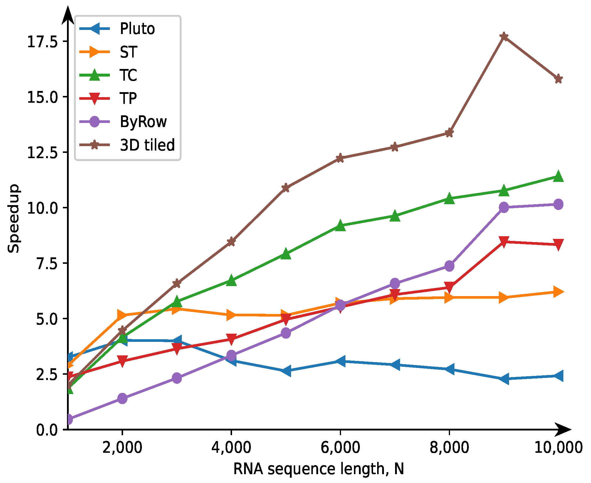
For shorter problem sizes, data are moved only among the different levels of cache, not to RAM, hence neither tiling approach allows for significant speedup of generated code [2]. Figure 2 depicts the speedup calculated on the basis of the times presented in Table 3. Under speedup we mean the ratio of the serial code execution time to the corresponding parallel code execution time. The second in terms of efficiency is the code generated with the correction approach implemented within the TRACO compiler. The ByRow code outperforms the codes generated with transpose and space-time tiling; the worst results are achieved for the code generated with Pluto, which is unable to tile the innermost loop nest.

Table 4. Time in seconds for Intel i7-8700 and N = 10,000 (ST, TC, and TP denote the codes generated on the basis of the space-time, tile correction, and transpose approaches, respectively).

Threads	Serial	Pluto	ST	TC	TP	ByRow	3D Tiled
1	1521.17	1564.28	796.16	437.59	584.25	486.25	312.38
2		902.88	453.24	236.73	310.54	271.70	217.58
4		657.66	307.04	165.55	206.75	160.11	119.01
8		643.33	255.08	155.50	198.03	160.13	100.71
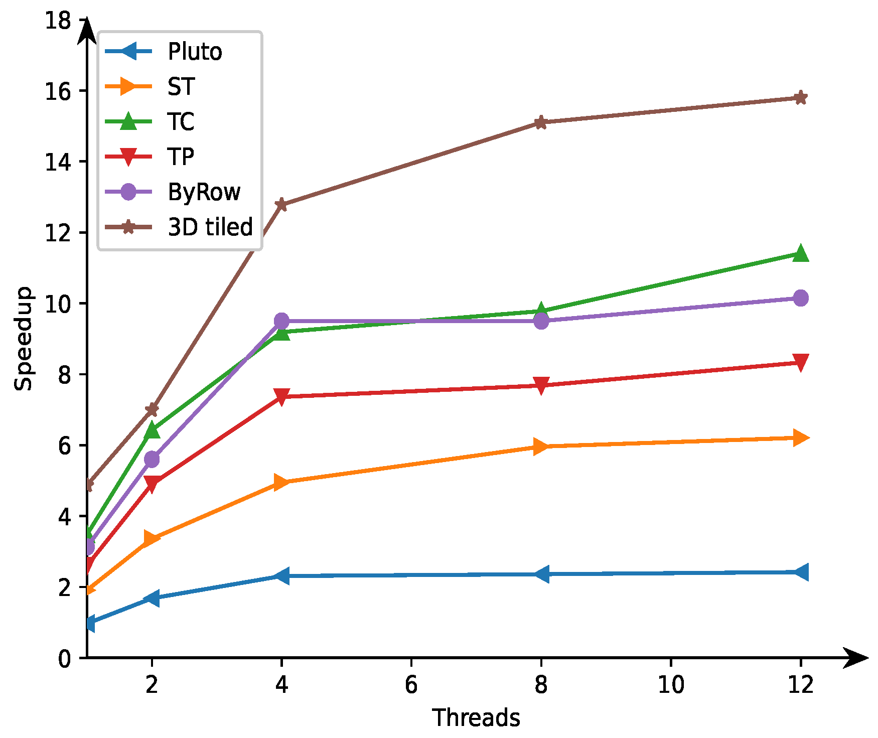
12		628.74	244.81	133.33	182.67	149.88	96.26

shows how the code execution times depend on the number of threads (1, 2, 4, 8, and 12) for N = 10,000 on the Intel i7-8700 processor. We can observe that the presented approach allows for (i) generation of scalable code (execution time decreases with the increasing number of treads) and (ii) achieving the highest code performance for each number of threads in comparison with that of the reminding examined codes. The second in terms of performance is the code obtained with the tile correction strategy. Figure 3 depicts how code speedup depends on the number of treads for N = 10,000; speedup is calculated on the basis of the data presented in Table 4.

Table 5. Time in seconds for Intel Xeon E5-2699 v3 and 36 threads (ST, TC, and TP denote the codes generated on the basis of the space-time, tile correction, and transpose approaches, respectively).

N	Serial	Pluto	ST	TC	TP	ByRow	3D tiled
1000	0.97	0.11	0.11	0.14	0.08	2.48	0.16
2000	14.15	1.16	0.70	0.69	0.42	3,33	0.63
3000	41.94	3.43	2.28	1.45	1.30	12.04	1.39
4000	142.88	6.61	5.66	3.61	4.59	27.46	2.54
5000	231.11	16.28	10.14	7.89	11.99	54.38	5.07
6000	383.21	29.17	17.98	15.51	23.83	106.89	6.97
7000	591.93	45.31	27.29	22.19	38.44	144.69	10.48
8000	885.61	65.32	41.33	35.51	56.41	213.79	14.65
9000	1646.16	91.22	58.77	48.72	80.49	329.83	21.77
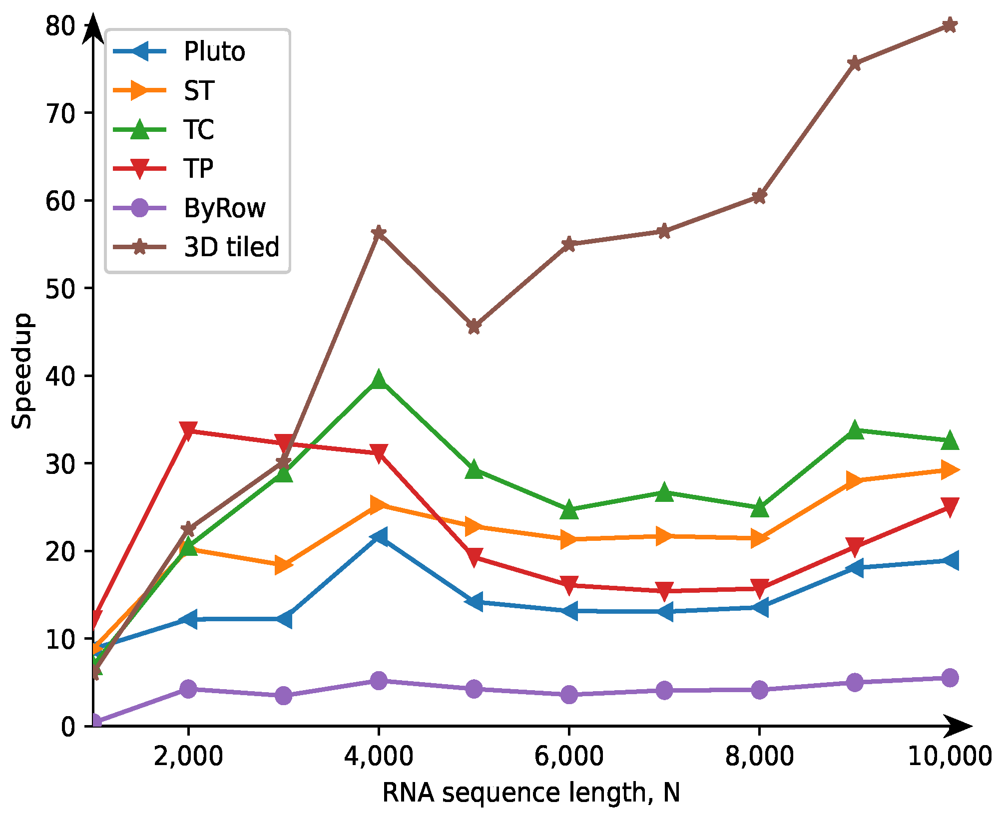
10,000	2447.72	129.41	83.64	75.11	97.91	443.29	30.41

presets execution times in seconds on Intel Xeon E5-2699 v3 and 36 threads used for code execution. The code generated with the approach presented in this article outperforms strongly the other examined codes starting from the problem size $N=3000$. For shorter RNA strands, the transpose code demonstrates better performance because, in such a case, there is no data moving between cache and RAM. For longer sequences, the 3D tiled code accelerates over eighty times the serial code and allows us to achieve super-linear speedup (greater than 36).

It is worth noting that for longer sequences, space-time tiling allows achieving higher performance on Intel Xeon than that achieved on i7-8700. On the other side, the ByRow code is not so efficient on Intel Xeon as on i7-8700. It is worth noting that for 36 threads, the parallel ByRow code does not outperform the serial ByRow code.

Code speedup calculated on the basis of the data in Table 5 are presented in Figure 4.

Table 6. Time in seconds for Intel Xeon E5-2699 v3 and RNA sequence length, N = 10,000 (ST is space time, TC is tile correction, TP is transpose).

threads	Serial	Pluto	ST	TC	TP	ByRow	3D Tiled
1	2447.7	2294.3	1069.2	561.97	947.87	1006.99	385.60
2		1318.1	493.1	466.67	444.11	807.20	262.86
4		783.8	240.3	274.29	242.85	685.91	144.41
8		445.5	131.4	148.34	134.46	518.30	86.46
16		250.7	95.1	93.50	119.52	466.54	53.18
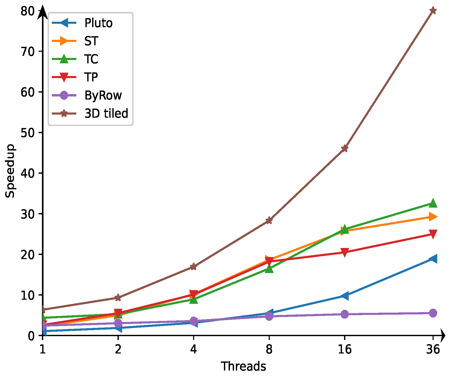
36		129.4	83.6	75.11	97.91	443.29	30.41

and Figure 5 present times and speedup on 1, 2, 4, 8, 16, and 36 threads, respectively, for the longest RNA length, $N=$ 10,000 under our experiments. As we can see, the performances of the serial and parallel 3D tiled codes are much greater than those achieved for the codes generated with the related approaches. The low speedup of the Byrow code is due to the fact that this code is not tiled and that the innermost loop is only parallelized.

6. Discussion

Two-dimensional tiles generated by means of well-known techniques implementing Nussinov’s algorithm and mentioned in Section 4 are unbounded along axis k. For such tiles, it is very difficult to choose a proper tile size, allowing for holding all data associated with a single 2D tile in cache. This reduces code locality. Whereas, 3D tiles generated by means of the approach proposed in this article are bounded along each axis, so, there is a possibility to choose a proper size for the 3D tile that allows us to hold all data associated with each tile in cache. This increases code locality that improves code performance. Summing up, we may conclude that the 3D serial and parallel tiled codes presented in this article allow us to achieve outstanding performance on the both computers used by us for experiments Intel i7-8700 (3.2 GHz, 6 cores, 12 threads, 12 MB cache, and Intel Xeon E5-2699 v3, 2.3 GHz (3.6 GHz turbo), 18 cores, 36 threads, 45 MB cache) for each number of threads (1 to 36) for larger problem sizes causing data moving between cache and RAM. Those codes outperform all of the examined, closely related codes.

7. Conclusions

This article introduces a new approach to generate 3D static parallel tiled code implementing Nussinov’s RNA folding. Increasing tile dimension from 2D to 3D allows us to considerably increase target code locality that leads to improving this code performance. Experiments carried out by us demonstrate that the generated 3D parallel tiled code outperforms all implementations known to us of Nussinov’s RNA folding and allows for obtaining super-linear code speedup for a larger RNA sequence length, i.e., the ratio of the serial code execution time to that of the parallel one exceeds the number of threads used for the parallel code execution. In the future, we intend to adapt the presented approach to other bioinformatics codes to generate tiled code of the enlarged tile dimension in comparison with state-of-the-art applications.