
Environment Classification Using Machine Learning Methods for Eco-Driving Strategies in Intelligent Vehicles

 ,
,  , , and
Abstract
:1. Introduction
2. Previous Works
2.1. Synergy Opportunities of New Technologies
2.2. Road Perception
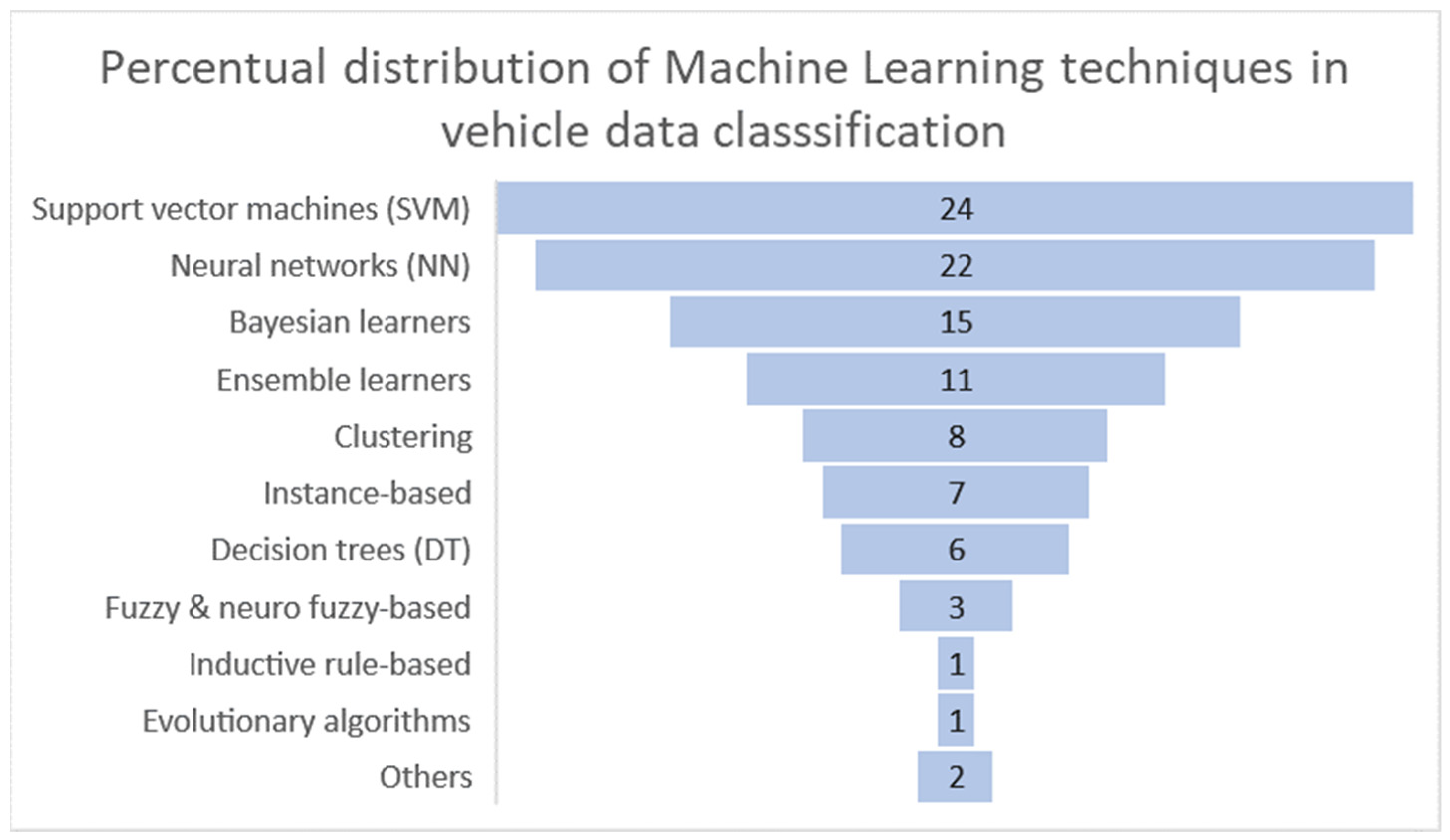
3. State of the Art
4. Methodology
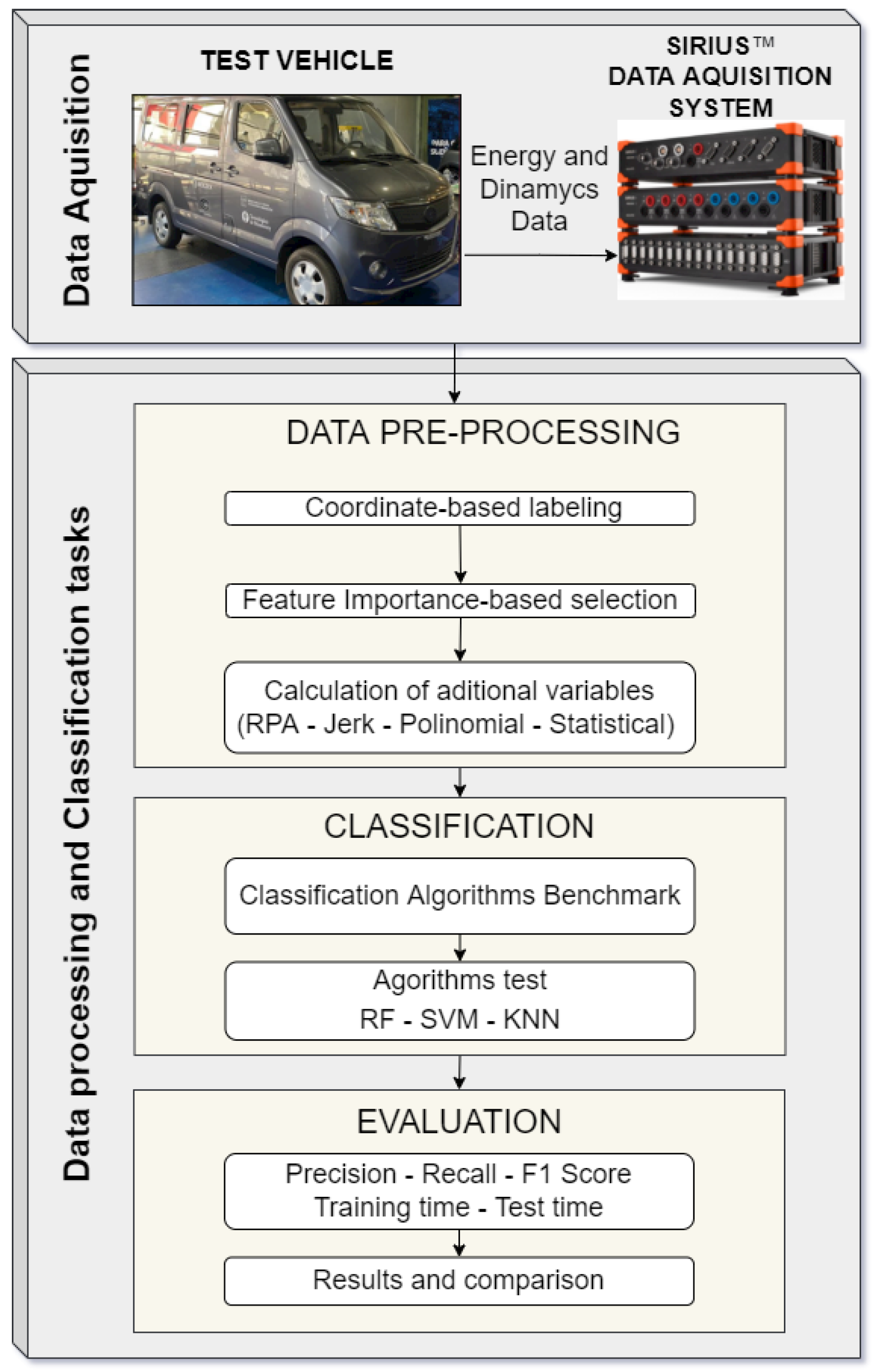
4.1. Work Process Overview
4.2. Experimentation and Test Route
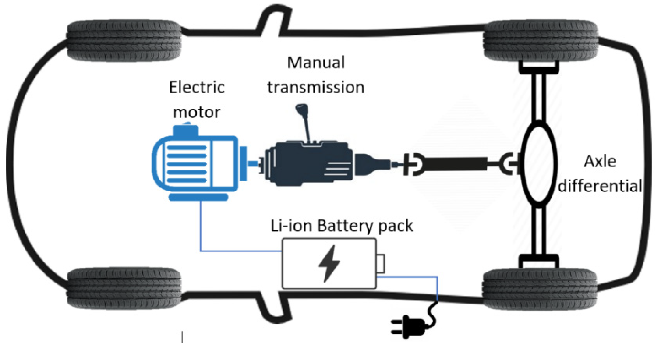
4.3. Test Vehicle
5. Features and Data Preparation
5.1. Data Pre-Processing
5.2. Variable’s Information and Features Analysis
5.2.1. Driver Effect in the Driving Environment Classification
5.2.2. Electric Power Variables
5.3. Data Processing and Environment Parameters
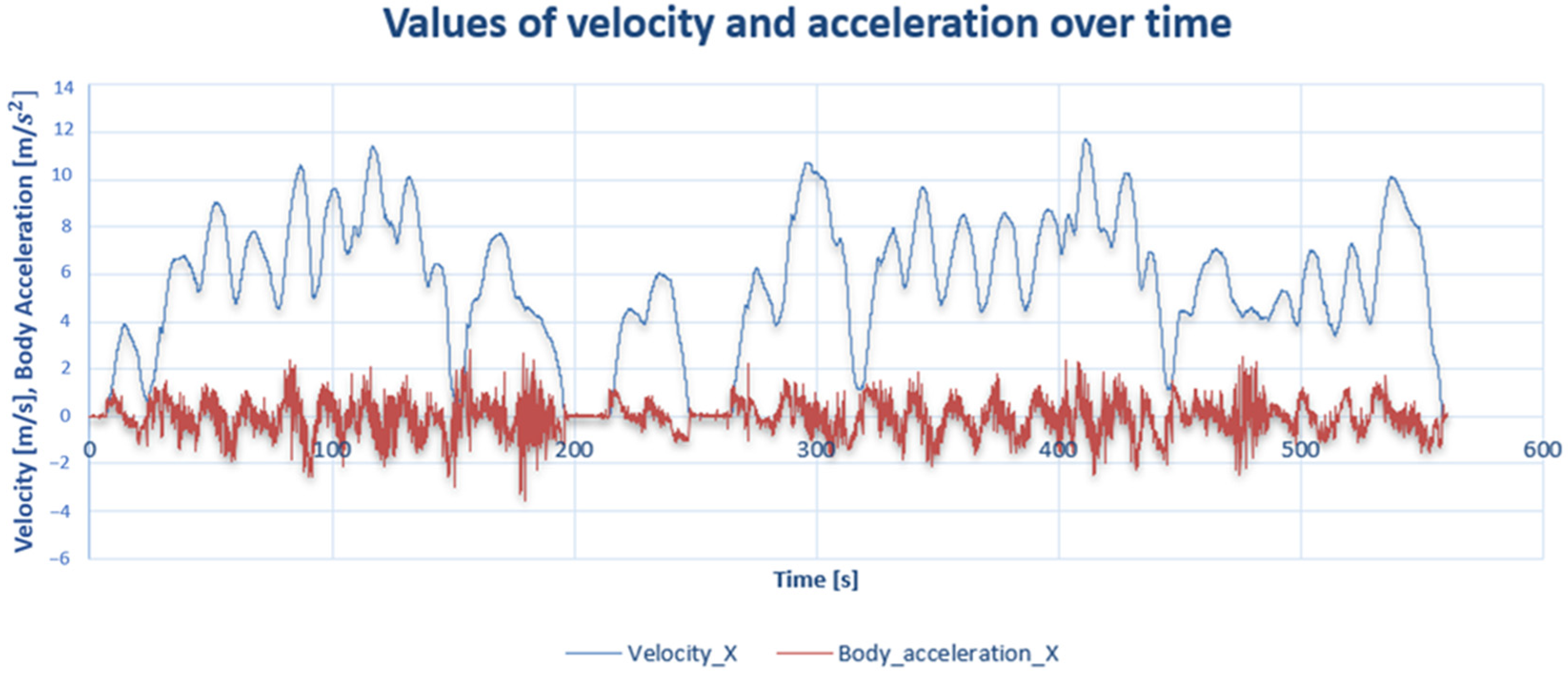
6. Data Analysis
6.1. Analysis of Samples from Pure Datasets
6.2. Data Segmentation into Subsamples
7. Results and Discussion
7.1. Feature Importance Results based on Mean Decrease in Impurity
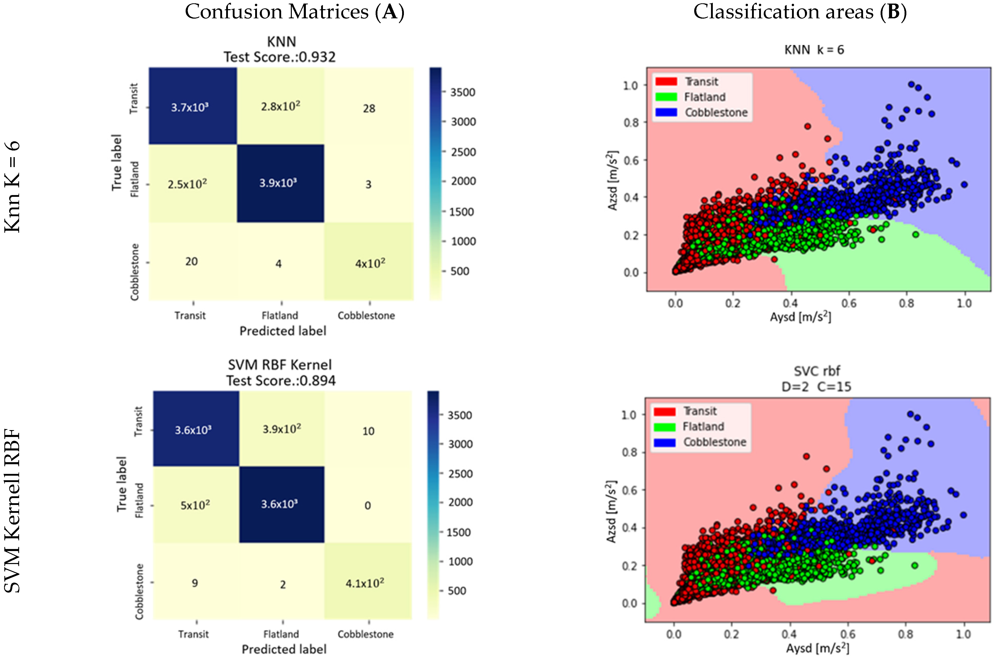
7.2. Classifiers Benchmark
7.3. Processing and Analysis of Samples in 2-s Windows
8. Conclusions
9. Future Work
- The integration of ML classifiers into intelligent driving systems for real-time awareness in pre-defined scenarios and the use of this information for calculating optimal energy-use strategies (Figure 15).
- The automatic classification of new scenarios, using ML strategies such as unsupervised learning for the clustering of classes with common characteristics in terms of drivability and energetic-related driving-style requirements.
- The same methodology exposed in this work can be tested again and improved by including more driving scenarios and routes with more complex characteristics and interactions with other players of the driving environment.
Author Contributions
Funding
Institutional Review Board Statement
Informed Consent Statement
Data Availability Statement
Acknowledgments
Conflicts of Interest
Appendix A

| Acronym | Definition |
|---|---|
| ML | Machine Learning |
| KNN | k-nearest neighbors |
| RF | Random Forest |
| SVC | Support Vector Classifier |
| SVM | Support Vector Machine |
| RBF | Radial Base Function |
| IMU | Inertial Measurement Unit |
| Feature Name | Description |
|---|---|
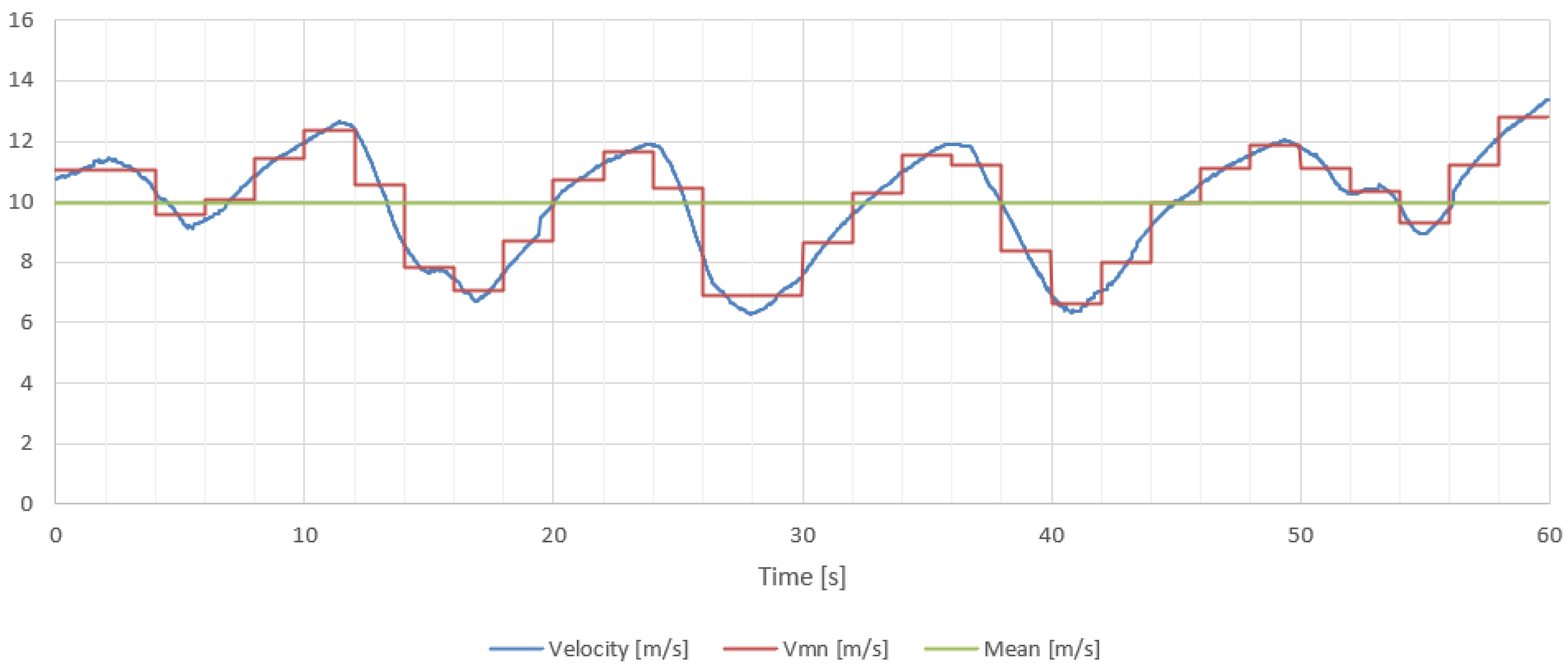
| Vmn [m/s] | Mean Longitudinal Velocity [44] |
| Vsd [m/s] | Standard deviation of longitudinal velocity [44] |
| Amn(+) [m/s2] | Mean of the positive acceleration in X. It is related to the use of the throttle [44] |
| Asd(+) | Standard deviation of positive acceleration at X [44] |
| Axsd [m/s2] | Standard deviation of longitudinal acceleration [44] |
| Axmn [m/s2] | Mean longitudinal acceleration [44] |
| Aymn [m/s2] | Mean of vertical acceleration |
| Aysd [m/s2] | Standard deviation of vertical acceleration |
| Azmn [m/s2] | Average lateral acceleration |
| Azsd [m/s2] | Standard deviation of lateral acceleration |
| Abrmn [m/s2] | Mean of braking acceleration (negative values of longitudinal acceleration) [44] |
| Abrsd | Standard deviation of braking acceleration [44] |
| RPA | Relative positive acceleration [38] |
| Potmn | Average power during the test, measured from batteries |
| Potsd | Standard deviation of electrical power |
| Jerk (X, Y, Z) [m/s3] | Statistical value for comfort, relates the standard deviation and the average of the signal derived from the acceleration in each of the coordinate axes [40] |
| Rollmn | Roll average |
| Rollsd | Roll standard deviation |
| Pitchmn | Pitch average |
| Pitchsd | Pitch standard deviation |
| Energy [Wh/km] | Electric energy measured at the motor, given for each kilometer travelled |
References
- Qi, X.; Barth, M.J.; Wu, G.; Boriboonsomsin, K.; Wang, P. Energy Impact of Connected Eco-Driving on Electric Vehicles. In Road Vehicle Automation 4; Springer: Cham, Switzerland, 2018; pp. 97–111. [Google Scholar] [CrossRef] [Green Version]
- Asher, Z.D.; Trinko, D.A.; Bradley, T.H. Increasing the Fuel Economy of Connected and Autonomous Lithium-Ion Electrified Vehicles. In Green Energy and Technology; Springer: Berlin/Heidelberg, Germany, 2018; pp. 129–151. [Google Scholar] [CrossRef]
- Shao, Y.; Sun, Z. Optimal Speed Control for a Connected and Autonomous Electric Vehicle Considering Battery Aging and Regenerative Braking Limits. In Proceedings of the ASME 2019 Dynamic Systems and Control Conference, Park City, UT, USA, 8–11 October 2019; Volume 1. [Google Scholar] [CrossRef]
- Urbanik, T.; Tanaka, A.; Lozner, B.; Lindstrom, E.; Lee, K.; Quayle, S.; Beaird, S.; Tsoi, S.; Ryus, P.; Gettman, D.; et al. Signal Timing Manual, 2nd ed.; Transportation Research Board: Washington, DC, USA, 2015. [Google Scholar] [CrossRef]
- Katrakazas, C.; Quddus, M.; Chen, W.H.; Deka, L. Real-Time Motion Planning Methods for Autonomous on-Road Driving: State-of-the-Art and Future Research Directions. Transp. Res. Part C Emerg. Technol. 2015, 60, 416–442. [Google Scholar] [CrossRef]
- Hellström, E.; Åslund Jan, J.; Nielsen, L. Design of an Efficient Algorithm for Fuel-Optimal Look-Ahead Control. Control. Eng. Pract. 2010, 18, 1318–1327. [Google Scholar] [CrossRef] [Green Version]
- Kamal, M.A.S.; Mukai, M.; Murata, J.; Kawabe, T. Ecological Vehicle Control on Roads with up-down Slopes. IEEE Trans. Intell. Transp. Syst. 2011, 12, 783–794. [Google Scholar] [CrossRef]
- Ding, F.; Jin, H. On the Optimal Speed Profile for Eco-Driving on Curved Roads. IEEE Trans. Intell. Transp. Syst. 2018, 19, 4000–4010. [Google Scholar] [CrossRef]
- Elamrani Abou Elassad, Z.; Mousannif, H.; al Moatassime, H.; Karkouch, A. The Application of Machine Learning Techniques for Driving Behavior Analysis: A Conceptual Framework and a Systematic Literature Review. Eng. Appl. Artif. Intell. 2020, 87, 103312. [Google Scholar] [CrossRef]
- Tian, J.; Chin, A.; Yanikomeroglu, H. Connected and Autonomous Driving. IT Prof. 2018, 20, 31–34. [Google Scholar] [CrossRef] [Green Version]
- Chen, Y.; Feng, G.; Wu, S.; Tan, X. A New Hybrid Model Predictive Controller Design for Adaptive Cruise of Autonomous Electric Vehicles. J. Adv. Transp. 2021, 2021, 6626243. [Google Scholar] [CrossRef]
- Kanjee, R.; Bachoo, A.K.; Carroll, J. Vision-Based Adaptive Cruise Control Using Pattern Matching. In Proceedings of the 2013 6th Robotics and Mechatronics Conference (RobMech), Durban, South Africa, 30–31 October 2013; pp. 93–98. [Google Scholar] [CrossRef]
- Bingham, C.; Walsh, C.; Carroll, S. Impact of Driving Characteristics on Electric Vehicle Energy Consumption and Range. IET Intell. Transp. Syst. 2012, 6, 29–35. [Google Scholar] [CrossRef]
- Ajanović, Z.; Stolz, M.; Horn, M. Energy Efficient Driving in Dynamic Environment: Considering Other Traffic Participants and Overtaking Possibility. In SpringerBriefs in Applied Sciences and Technology; Springer: Berlin/Heidelberg, Germany, 2017; pp. 61–80. [Google Scholar] [CrossRef]
- Bae, S.; Kim, Y.; Guanetti, J.; Borrelli, F.; Moura, S. Design and Implementation of Ecological Adaptive Cruise Control for Autonomous Driving with Communication to Traffic Lights. In Proceedings of the 2019 American Control Conference (ACC), Philadelphia, PA, USA, 10–12 July 2019; pp. 4628–4634. [Google Scholar] [CrossRef] [Green Version]
- Shao, Y.; Mohd Zulkefli, M.A.; Sun, Z.; Huang, P. Evaluating Connected and Autonomous Vehicles Using a Hardware-in-the-Loop Testbed and a Living Lab. Transp. Res. Part C Emerg. Technol. 2019, 102, 121–135. [Google Scholar] [CrossRef]
- Hellström, E.; Ivarsson, M.; Åslund, J.; Nielsen, L. Look-Ahead Control for Heavy Trucks to Minimize Trip Time and Fuel Consumption. Control. Eng. Pract. 2009, 17, 245–254. [Google Scholar] [CrossRef] [Green Version]
- Škugor, B.; Deur, J. Synthetic Driving Cycles-Based Modelling of Extended Range Electric Vehicle Fleet Energy Demand. In Proceedings of the 30th International Electric Vehicle Symposium & Exhibition (EVS30), Stuttgart, Germany, 9–11 October 2018. [Google Scholar]
- Teng, G.; Xiao, J.; He, Y.; Zheng, T.; He, C. Use of Group Method of Data Handling for Transport Energy Demand Modeling. Energy Sci. Eng. 2017, 5, 302–317. [Google Scholar] [CrossRef]
- Brand, C.; Anable, J.; Morton, C. Lifestyle, Efficiency and Limits: Modelling Transport Energy and Emissions Using a Socio-Technical Approach. Energy Effic. 2019, 12, 187–207. [Google Scholar] [CrossRef] [Green Version]
- De Cauwer, C.; Verbeke, W.; Coosemans, T.; Faid, S.; van Mierlo, J. A Data-Driven Method for Energy Consumption Prediction and Energy-Efficient Routing of Electric Vehicles in Real-World Conditions. Energies 2017, 10, 608. [Google Scholar] [CrossRef] [Green Version]
- Delogu, M.; del Pero, F.; Pierini, M. Lightweight Design Solutions in the Automotive Field: Environmental Modelling Based on Fuel Reduction Value Applied to Diesel Turbocharged Vehicles. Sustainability 2016, 8, 1167. [Google Scholar] [CrossRef] [Green Version]
- Topić, J.; Škugor, B.; Deur, J. Neural Network-Based Modeling of Electric Vehicle Energy Demand and All Electric Range. Energies 2019, 12, 1396. [Google Scholar] [CrossRef] [Green Version]
- Zeiler, M.D.; Fergus, R. Visualizing and Understanding Convolutional Networks. In Computer Vision—ECCV 2014, Proceedings of the 13th European Conference, Zurich, Switzerland, 6–12 September 2014; Lecture Notes in Computer Science (Including Subseries Lecture Notes in Artificial Intelligence and Lecture Notes in Bioinformatics); Springer: Berlin/Heidelberg, Germany, 2014; Volume 8689, pp. 818–833. [Google Scholar] [CrossRef] [Green Version]
- Tian, Y.; Pei, K.; Jana, S.; Ray, B. DeepTest: Automated Testing of Deep-Neural-Network-Driven Autonomous Cars. In Proceedings of the 2018 IEEE/ACM 40th International Conference on Software Engineering (ICSE), Gothenburg, Sweden, 27 May–3 June 2018; pp. 303–314. [Google Scholar] [CrossRef]
- Min, K.; Yeon, K.; Jo, Y.; Sim, G.; Sunwoo, M.; Han, M. Vehicle Deceleration Prediction Based on Deep Neural Network at Braking Conditions. Int. J. Automot. Technol. 2020, 21, 91–102. [Google Scholar] [CrossRef]
- Jonas, T.; Hunter, C.D.; Macht, G.A. Quantifying the Impact of Traffic on Electric Vehicle Efficiency. World Electr. Veh. J. 2022, 13, 15. [Google Scholar] [CrossRef]
- Wang, J.; Meng, Q.; Shang, P.; Saada, M. Road surface real-time detection based on Raspberry Pi and recurrent neural networks. Trans. Inst. Meas. Control. 2021, 43, 2540–2550. [Google Scholar] [CrossRef]
- Lei, T.; Mohamed, A.A.; Claudel, C. An IMU-based traffic and road condition monitoring system. HardwareX 2018, 4, e00045. [Google Scholar] [CrossRef]
- Trogh, J.; Botteldooren, D.; de Coensel, B.; Martens, L.; Joseph, W.; Plets, D. Map Matching and Lane Detection Based on Markovian Behavior, GIS, and IMU Data. IEEE Trans. Intell. Transp. Syst. 2020, 23, 2056–2070. [Google Scholar] [CrossRef]
- Orfila, O.; Gruyer, D.; Hamdi, K.; Glaser, S. Safe and Ecological Speed Profile Planning Algorithm for Autonomous Vehicles Using a Parametric Multiobjective Optimization Procedure. Accepted. Int. J. Automot. Eng. 2019, 10, 26–33. [Google Scholar] [CrossRef] [Green Version]
- Hu, Y.; Li, W.; Xu, K.; Zahid, T.; Qin, F.; Li, C. Energy Management Strategy for a Hybrid Electric Vehicle Based on Deep Reinforcement Learning. Appl. Sci. 2018, 8, 187. [Google Scholar] [CrossRef] [Green Version]
- Jeoung, H.; Lee, K.; Kim, N. Methodology for finding maximum performance and improvement possibility of rule-based control for parallel type-2 hybrid electric vehicles. Energies 2019, 12, 1924. [Google Scholar] [CrossRef] [Green Version]
- Kazemi, H.; Mahjoub, H.N.; Tahmasbi-Sarvestani, A.; Fallah, Y.P. A Learning-based Stochastic MPC Design for Cooperative Adaptive Cruise Control to Handle Interfering Vehicles. IEEE Trans. Intell. Veh. 2018, 3, 266–275. [Google Scholar] [CrossRef] [Green Version]
- Rasool, E.; Liaquat, M.; Bhatti, A.I.; Mehmood, A. Cooperative Adaptive Cruise Control with Fuel Efficiency Using PMP Technique. In Proceedings of the 2019 5th International Conference on Control, Automation and Robotics (ICCAR 2019), Beijing, China, 19–22 April 2019; pp. 396–400. [Google Scholar] [CrossRef]
- Delnevo, G.; di Lena, P.; Mirri, S.; Prandi, C.; Salomoni, P. On combining Big Data and machine learning to support eco-driving behaviours. J. Big Data 2019, 6, 64. [Google Scholar] [CrossRef] [Green Version]
- Zhu, J.; Ngo, C.; Sciarretta, A. Real-Time Optimal Eco-Driving for Hybrid-Electric Vehicles. IFAC-PapersOnLine 2019, 52, 562–567. [Google Scholar] [CrossRef]
- Tutuianu, M.; Bonnel, P.; Ciuffo, B.; Haniu, T.; Ichikawa, N.; Marotta, A.; Pavlovic, J.; Steven, H. Development of the World-Wide Harmonized Light Duty Test Cycle (WLTC) and a Possible Pathway for Its Introduction in the European Legislation. Transp. Res. Part D: Transp. Environ. 2015, 40, 61–75. [Google Scholar] [CrossRef]
- Van de Weijer, C.J.T. Heavy-Duty Emission Factors: Development of Representative Driving Cycles and Prediction of Emissions in Real-Life. Ph.D. Thesis, Technischen Universität Graz, Graz, Austria, 1997. [Google Scholar]
- Murphey, Y.L.; Milton, R.; Kiliaris, L. Driver’s Style Classification Using Jerk Analysis. In Proceedings of the 2009 IEEE Workshop on Computational Intelligence in Vehicles and Vehicular Systems, Nashville, TN, USA, 30 March–2 April 2009; pp. 23–28. [Google Scholar] [CrossRef]
- MATLAB Documentation. Available online: https://www.mathworks.com/help/matlab/ (accessed on 4 April 2022).
- Pedregosa, F.; Varoquaux, G.; Gramfort, A.; Michel, V.; Thirion, B.; Grisel, O.; Blondel, M.; Prettenhofer, P.; Weiss, R.; Dubourg, V. Scikit-Learn: Machine Learning in Python. J. Mach. Learn. Res. 2011, 12, 2825–2830. [Google Scholar]
- Buitinck, L.; Louppe, G.; Blondel, M.; Pedregosa, F.; Müller, A.C.; Grisel, O.; Niculae, V.; Prettenhofer, P.; Gramfort, A.; Grobler, J.; et al. API Design for Machine Learning Software: Experiences from the Scikit-Learn Project. arXiv 2013, arXiv:1309.0238. [Google Scholar] [CrossRef]
- Constantinescu, Z.; Marinoiu, C.; Vladoiu, M. Driving Style Analysis Using Data Mining Techniques. Int. J. Comput. Commun. Control 2010, 5, 654. [Google Scholar] [CrossRef]


| Article | Authors | Functions | Model | Methods | Evaluation |
|---|---|---|---|---|---|
| Increasing the Fuel Economy of Connected and Autonomous Lithium-Ion Electrified Vehicles | Asher et al., 2018 [2] | Energy Management, V2V, environment Perception | Vehicle Dynamics Model, Energy Management Model | Dynamic programming and Pontryagin’s Minimization Principle | SIMULATION using models to compare results of different control strategies |
| On the Optimal Speed Profile for Eco-Driving on Curved Roads | Ding et al., 2019 [8] | Velocity profile optimization for curved roads | Vehicle Dynamics Model, Fuel Consumption Model | Dynamic programming Optimization | Algorithm verification using co-simulation of CarSim and Matlab/Simulink |
| Design and Implementation of Ecological Adaptive Cruise Control for Autonomous Driving with Communication to Traffic Lights | Bae et al., 2018 [15] | V2I, EAD *, Surrounding traffic consideration | Vehicle Dynamics Model | Robust Model Predictive Control | ACC ** tested in a Hardware in the Loop setup with SPaT *** information |
| Vehicle Deceleration Prediction Based on Deep Neural Network at Braking Conditions | Min et al., 2020 [26] | Decelerations predictions | Deep learning | Deep neural network (RNN, LSTM, conventional neural network), K means clustering method | Vehicle velocity, relative distance between the vehicle and the traffic light, reference acceleration |
| Quantifying the Impact of Traffic on Electric Vehicle Efficiency | Jonas et al., 2022 [27] | Impact of traffic on Electric Vehicle efficiency | Statistical models | Regression models, ANOVA | Total energy consumption, total distance, Average consumption per mile, Mean variation in speed, Mean variation in acceleration, Mean variation in jerk |
| Road surface real-time detection based on Raspberry Pi and recurrent neural networks | Wang et al., 2021 [28] | Road surface detection | Recurrent Neural Network | Allan variance, Machine learning algorithms (KNN, L2 logistic regression, Decision tree, SVM cross validation), Deep learning Algorithms (LSTM, RNN) | Three axis accelerometer (x, y, z) and three axis gyroscope (x, y, z) |
| An IMU-based traffic and road condition monitoring system | Lei et al., 2018 [29] | Traffic and road condition monitoring system | Fast Fourier Transform | Least squares optimization for speed estimation considering sensor bias, DCM filter for attitude angle estimation | Relation between vertical acceleration and Present Serviceability Rating (PSR) |
| Map Matching and Lane Detection Based on Markovian Behavior, GIS, and IMU Data | Trogh et al., 2020 [30] | Map matching and lane detection | Markovian behavior | Viterbi (hidden Markov model) | Direction of road segments, maximum allowed speed per road segment, and driving behavior |
| Safe and Ecological Speed Profile Planning Algorithm for Autonomous Vehicles Using a Parametric Multi-objective Optimization Procedure | Orfila et al., 2019 [31] | Velocity profile optimization for predefined route | Data-driven approach | Global Optimization using Simulated Annealing | Velocity profile data comparison—Algorithm results Vs human drivers experimental data |
| Energy Management Strategy for a Hybrid Electric Vehicle Based on Deep Reinforcement Learning | Hu et al., 2018 [32] | Energy Management | HEV Model | Deep Reinforcement Learning | Trained control Algorithm tested in MATHLAB and ADVISOR Co-simulation |
| Methodology for Finding Maximum Performance and Improvement Possibility of Rule-Based Control for Parallel Type-2 Hybrid Electric Vehicles | Jeoung et al., 2019 [33] | Rule based controller, Energy Management | Parallel Type 2 HEV Model | Dynamic programming and Pontryagin’s Minimization Principle | Controller algorithm evaluation in SIMULATION HEV MODEL |
| A Learning-Based Stochastic MPC Design for Cooperative Adaptive Cruise Control to Handle Interfering Vehicles | Kazemi et al., 2018 [34] | CACC, Surrounding traffic consideration, V2V | Data-driven approach | Artificial Neural Network | Model Predictive Controller evaluated in SIMULATED test runs from a real driving tests dataset |
| Cooperative Adaptive Cruise Control with Fuel Efficiency Using PMP Technique | Rasool et al., 2019 [35] | CACC, Surrounding traffic consideration | Platoon model, ICE power train Model | Pontryagin’s Minimization Principle | Validation of the controller with the models in a SIMULATION |
| On combining Big Data and machine learning to support eco-driving behaviors | Delnevo et al., 2019 [36] | HMI, ADAS | Data-driven approach | Machine Learning | Algorithm testing in SIMULATION using real data |
| Real-Time Optimal Eco-Driving for Hybrid-Electric Vehicles | Zhu et al., 2019 [37] | ADAS, HEV | Data-driven approach | Dynamic programming Optimization/Artificial Neural Network | Mutual Validation of the obtained speed profiles using DPO and ANN methods |
| Environment classification using machine learning methods for eco-driving strategies in intelligent vehicles. | (THIS PROPOSED WORK) | Driving Environment classification | Machine learning models | Machine Learning algorithms (KNN, SVM, Decision tree) | Linear velocity, three axis acceleration, energy consumption, jerk, roll, pitch |
| Motor | |
| Power | 15 HP |
| Nominal Voltage | 76 V |
| Nominal current | 115 A |
| Peak current | 132 A |
| Max speed | 3000 RPM |
| Battery | |
| Total voltage | 96 V |
| Number of cells | 32 |
| Total Energy Capacity | 28,800 Wh |
| Discharge rating 2C | 0.5 |
| Discharge current | 150 A |
| Vehicle brute mass | 1370 kg |
| Wheels’ dynamic radius | 0.25019 m |
| Rolling resistance coefficient | 0.014984 |
| Aerodynamic drag coefficient | 0.436 |
| Vehicle frontal Area | 2.15 m2 |
| Gearbox efficiency | 0.95 |
| Axle differential efficiency | 0.95 |
| Top Speed | 100 km/h |
| KNN F1-Score | SVM F1-Score | Support Samples | |
|---|---|---|---|
| Flatland | 0.8 | 0.99 | 45 |
| Cobblestone | 0.7 | 1.0 | 36 |
| Transit | 0.88 | 0.99 | 38 |
| Accuracy | 0.8 | 0.99 | 119 |
| Macro avg. | 0.8 | 0.99 | 119 |
| KNN k = 19 | SVM (RBF) | Random Forest | |
|---|---|---|---|
| Test accuracy | 93.2% | 88.9% | 90.7% |
| Precision | 93% | 89% | 91% |
| Recall | 94% | 89% | 91% |
| F1-score | 93% | 89% | 91% |
| Support samples | 8535 | 8535 | 8535 |
Publisher’s Note: MDPI stays neutral with regard to jurisdictional claims in published maps and institutional affiliations. |
© 2022 by the authors. Licensee MDPI, Basel, Switzerland. This article is an open access article distributed under the terms and conditions of the Creative Commons Attribution (CC BY) license (https://creativecommons.org/licenses/by/4.0/).
Share and Cite
Julio-Rodríguez, J.d.C.; Rojas-Ruiz, C.A.; Santana-Díaz, A.; Bustamante-Bello, M.R.; Ramirez-Mendoza, R.A. Environment Classification Using Machine Learning Methods for Eco-Driving Strategies in Intelligent Vehicles. Appl. Sci. 2022, 12, 5578. https://doi.org/10.3390/app12115578
Julio-Rodríguez JdC, Rojas-Ruiz CA, Santana-Díaz A, Bustamante-Bello MR, Ramirez-Mendoza RA. Environment Classification Using Machine Learning Methods for Eco-Driving Strategies in Intelligent Vehicles. Applied Sciences. 2022; 12(11):5578. https://doi.org/10.3390/app12115578
Chicago/Turabian StyleJulio-Rodríguez, Jose del C., Carlos A. Rojas-Ruiz, Alfredo Santana-Díaz, M. Rogelio Bustamante-Bello, and Ricardo A. Ramirez-Mendoza. 2022. "Environment Classification Using Machine Learning Methods for Eco-Driving Strategies in Intelligent Vehicles" Applied Sciences 12, no. 11: 5578. https://doi.org/10.3390/app12115578