Linear Proportional-Integral-Differential-Robustified Continuous-Time Optimal Predictive Control for a Class of Nonlinear Systems

Abstract

This paper presents a novel robust optimal predictive control approach for a class of nonlinear continuous-time systems perturbed by unknown disturbances. First, a new error state with a linear proportional-integral-differential (PID) structure considering current, accumulative, and derivative tracking errors is defined. Second, prediction of the error state within the predictive periods is expressed by the error state and its high-order derivatives according to the Taylor series expansion. Last, the proposed control law as well as the main result of this paper are derived by minimizing the prediction of the error state. Numerical validation for designing a missile autopilot shows that, due to minimizing the accumulative tracking error included in the PID-structuralized new error state, the proposed approach can generate smaller steady-state tracking errors than two commonly applied continuous-time optimal predictive control approaches whether the disturbances encountered by the missile are constant or time-varying.

1. Introduction

Control design for nonlinear systems has always been a challenging task. Generally, the control approaches can be classified into linear and nonlinear catalogs. In the linear approaches, by simplifying or even neglecting partial nonlinearities, the systems are linearized around equilibrium points such that the classical and modern linear control theories [1,2] are applicable. However, in order to give consideration of the nonlinearities as much as possible to meet the increasing demand of high-quality control performances, various nonlinear control approaches such as the feedback linearization [3], the sliding mode control [4], the adaptive methodology [5], the finite time control [6], the backstepping approach [7], and so forth have been proposed and applied.

As a promising and viable nonlinear control approach, the continuous-time optimal predictive control (CTOPC) methodology [8] extends a novel prospect for the control design of the nonlinear systems. In the prototype CTOPC (PCTOPC), state of the dynamical system or the prescribed reference is predicted by a linear combination of its high-order derivatives by means of the Taylor series expansion. Then, the optimal predictive control law is obtained by minimizing a quadratic receding horizon performance index (RHPI), which is the function of the predictive response errors. The control law has the merit of giving full consideration of all the system nonlinearities due to the complete inclusion of the system dynamics, which makes the PCTOPC more attractive and have many successful applications in various fields during the past decades such as the flight control [9,10], the permanent magnet synchronous motor control [11], angle tracking control of a steer-by-wire system [12], the DC-DC converter control [13,14,15], the photovoltaic inverter control [16,17], the wind energy system design [18,19], the water tank system design [20,21], the active suspension system design [22], stabilization of an artificial gas-lift process [23], path following system design of autonomous mobile vehicles [24,25], and solar power plant control [26]. Though the PCTOPC has drawn much attention in the aforementioned areas, its inadequacy is also obvious. That is, the closed-loop system is susceptible to the unknown external uncertainties since the PCTOPC only takes into account of the current tracking errors between the prescribed reference and the system output, making poor robustness and large steady-state tracking errors easy to occur. Thus far, only few previous works have been dedicated to address such problems [9,19,21,23,24,25,26]. Therefore, targeting the inadequacy and extending an alternative methodology to enhance the robustness of the PCTOPC are meaningful and of engineering significance.

As one of the most widely used approaches around the world, the linear proportional-integral-differential (PID), which not only has the merits of simple controller structure and easy implementation procedures, but also has the strong capability on dealing with the unknown disturbances, has many successful application examples in various fields [27,28,29]. In the PID, considering the terms of accumulative tracking errors can help the closed-loop systems reduce stead-state errors. By assigning appropriate proportional, integral, and differential gain coefficients, satisfactory system response time and input performance can be acquired. Hence, the PID approach has been successfully applied to enhance the system robustness for the existing approaches [30,31]. Due to those advantages, this paper combines the PCTOPC with the linear PID approach for closed-loop system robustness enhancement. Next, the proposed approach is named as PID-CTOPC.

To further highlight superiorities of the proposed approach, comparison with another typical CTOPC approach [32,33], which considers both current and high-derivative tracking errors proposed by Professor Lu, is also conducted. The main contributions of this paper are twofold.

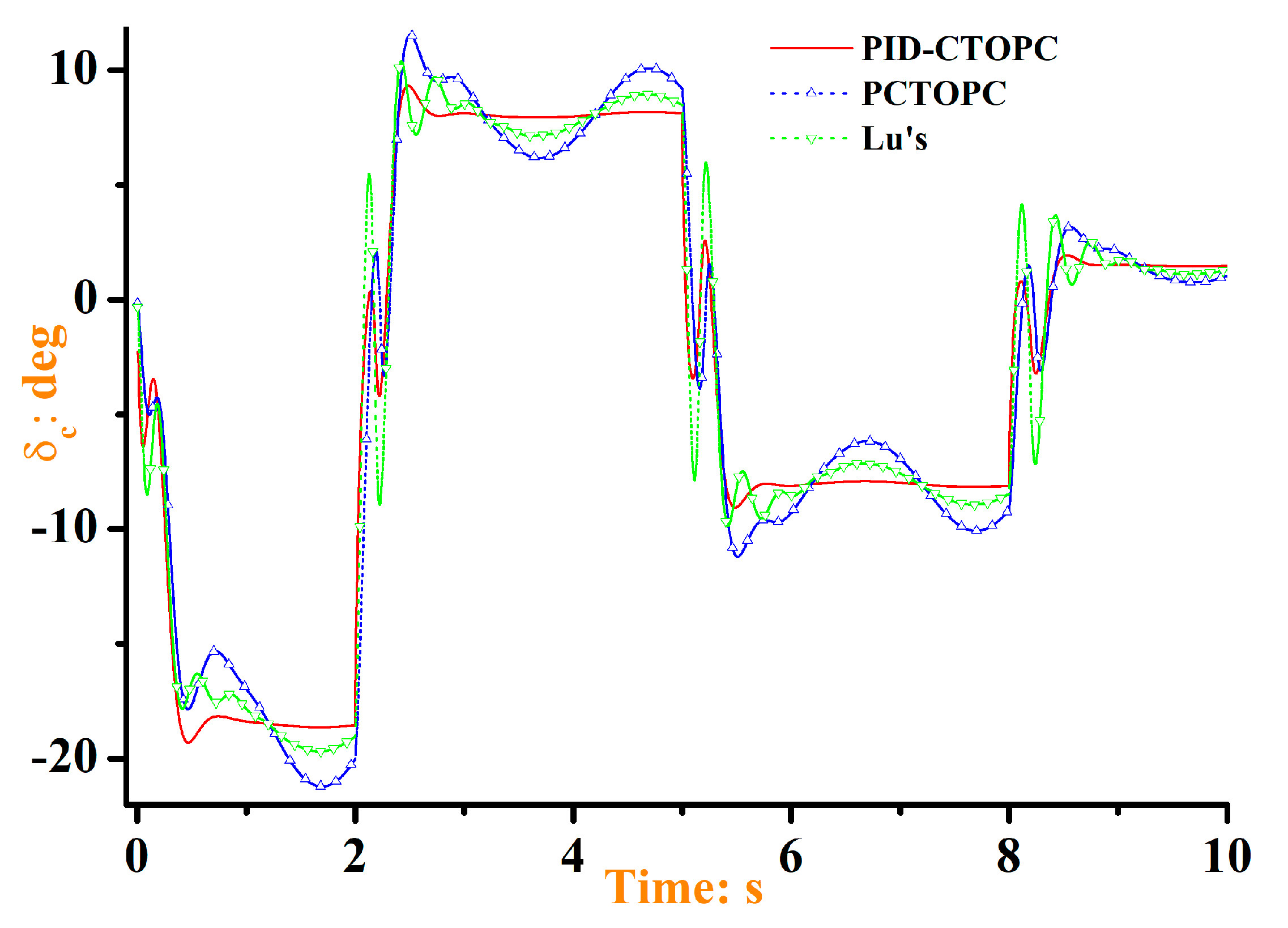
• A closed-loop steady-state tracking error reduction approach is proposed in the field of CTOPC. The accumulative tracking errors, which are integrated into a new error state with PID structure, are considered in the proposed PID-CTOPC approach such that tracking errors within the operation envelop of the closed-loop system can be minimized compared with the PCTOPC and the Lu’s approach, which only consider the current tracking errors.
• Robustness of the closed-loop system is significantly enhanced. In the proposed PID-CTOPC approach, current, accumulative, and derivative tracking errors are minimized simultaneously such that reduction of input fluctuation, output overshoot, and steady-state tracking error can also be derived in contrast with the PCTOPC and the Lu’s approach in the presence of unknown disturbances.

2. Preliminaries

In this section, some useful preliminaries such as symbols, lemmas, and existing optimal predictive approaches are introduced first.

Denote ${\mathbb{Z}}^{+}$ as the set of positive integers, $\mathbb{Z}=\left\{0,{\mathbb{Z}}^{+}\right\}$, $ℝ$ as the set of real numbers, ${ℝ}^{p\times q}$ as the set of $p\times q$ real matrices, ${ℝ}^s$ as the set of column matrices with dimension $s$, $O^{m\times n}$ as the set of $m\times n$ zero matrices, $s^{\left[j\right]}$ as the jth derivative of $s$ relative to time, $s!$ as the factorial of $s\in \mathbb{Z}$.

This paper considers the following single-input–single-output (SISO) nonlinear affine systems:

$$\{\begin{array}{l}{\stackrel{·}{x}}_i\left(t\right)=x_{i+1}\left(t\right), i=1,\dots ,n-1\\ {\stackrel{·}{x}}_n\left(t\right)=f\left(x\left(t\right)\right)+g\left(x\left(t\right)\right)\cdot u\left(t\right)\\ y\left(t\right)=x_1\left(t\right)\end{array}$$

(1)

where, $x\left(t\right)=\left[x_1\left(t\right),\dots ,x_n\left(t\right)\right]\in {ℝ}^n$ represents the state vector, $n\ge 2$ represents the system dimension. $y\left(t\right)\in ℝ$ and $u\left(t\right)\in ℝ$ represent output and input, respectively. $f\left(x\left(t\right)\right)\in ℝ$ and $g\left(x\left(t\right)\right)\in ℝ$ are nonlinear mappings with $g\left(x\right)\ne 0$ for any $x\left(t\right)$. In next, the variable $\vartheta \left(t\right)$ is denoted as $\vartheta$ while the prediction of $\vartheta$ within the predictive period $\tau >0$ would be expressed by $\vartheta \left(t+\tau \right)$, $\vartheta$ is a scalar or vector. The following assumptions are imposed on system (1):

(A1)

The zero dynamics are stable.

(A2)

All the states $x_i$, $i=1,\dots ,n$ are available.

(A3)

The system output $y$ and the prescribed reference $y_d$ are sufficiently many times continuously differentiable relative to time $t$.

Secondly, the PCTOPC approach is reviewed.

Differentiating both sides of the last state differential equation in Formula (1) $\sigma$ times relative to $t$ yields:

$$\{\begin{array}{l}{y}^{\left[n+1\right]}=p_1\left(u^2,u;x\right)+g\left(x\right)\cdot \stackrel{·}{u}\\ y^{\left[n+2\right]}=p_2\left(u^3,u^2,u,\stackrel{·}{u};x\right)+g\left(x\right)\cdot \stackrel{··}{u}\\ ⋮\\ y^{\left[n+\sigma \right]}=p_{\sigma }\left(u^{\sigma +1},\dots ,u,u^{\left[\sigma -1\right]},\dots ,\stackrel{·}{u};x\right)+g\left(x\right)\cdot u^{\left[\sigma \right]}\end{array}$$

(2)

where, $\sigma \in {\mathbb{Z}}^{+}$ is called control order. Details of the nonlinear terms $p_i$, $i=1,\dots ,\sigma$ can be seen in [8].

By using the Taylor series expansion, predictions of $y$ and $y_d$ within the predictive period $t_C$ can be expressed by:

$$\{\begin{array}{l}y\left(t+\tau \right)={\mathrm{\Gamma }}_c\cdot Y_c\\ y_d\left(t+\tau \right)={\mathrm{\Gamma }}_c\cdot Y_{cd}\end{array}$$

(3)

where, $0<\tau \le t_C$, ${\mathrm{\Gamma }}_c=\left[1,\tau ,\dots ,\frac{{\tau }^{n+\sigma }}{\left(r+\sigma \right)!}\right]$, $Y_c\left(t\right)={\left[y,\stackrel{·}{y},\dots ,y^{\left[n+\sigma \right]}\right]}^T$, and $Y_{cd}\left(t\right)={\left[y_d,{\stackrel{·}{y}}_d,\dots ,y_d^{\left[n+\sigma \right]}\right]}^T$.

By employing following RHPI:

$$J_C=\frac{1}{2}{{\displaystyle {\int }_0^{t_C}\left[y\left(t+\tau \right)-y_d\left(t+\tau \right)\right]}}^T\left[y\left(t+\tau \right)-y_d\left(t+\tau \right)\right]d\tau$$

(4)

the optimal predictive control law for the system (1) is summarized in following lemma.

 Lemma 1 

[8]. Consider the nonlinear affine system (1) satisfying (A1)~(A3). Then, for a given control order $\sigma \in {\mathbb{Z}}^{+}$, the system output  $y$  and the prescribed reference   $y_d$ are predicted by Formula (3). The optimal predictive control law minimizing the RHPI (4) is given by:

$$u\left(t\right)={\left[g\left(x\right)\right]}^{-1}\left[y_d^{\left[n\right]}-f\left(x\right)-K_c{M}_r\right]$$

(5)

where, $M_r$  is given by:

$$M_r={\left[x_1-y_d,x_2-{\stackrel{·}{y}}_d,\dots ,x_n-y_d^{\left[n-1\right]}\right]}^T$$

(6)

$K_c\in {ℝ}^{1\times \left(\sigma +1\right)}$is the first row of matrix  $A_{\sigma }^{-1}{A}_1$ . The matrices  $A_1$ and  $A_{\sigma }$ are given by:

$$\{\begin{array}{l}A={\displaystyle {\int }_0^{t_1}{\mathrm{\Gamma }}_c^T{\mathrm{\Gamma }}_{c}d\tau }=\left[\begin{array}{cc}{A}_r& A_1^T\\ A_1& A_{\sigma }\end{array}\right]\in {ℝ}^{\left(n+\sigma +1\right)\times \left(n+\sigma +1\right)}\\ A_r\in {ℝ}^{n\times n}, A_{\sigma }\in {ℝ}^{\left(\sigma +1\right)\times \left(\sigma +1\right)}\end{array}$$

(7)

3. The PID-CTOPC Approach

This section presents main results of this paper. Firstly, a new error state with PID structure is introduced, transforming the prescribed reference tracking problem into a stabilization one for the system (1). Secondly, the robustified optimal predictive controller is designed.

3.1. Stabilization Model

A new error state with PID structure is defined as follows:

$$s\left(t\right)=K_p{e}_1+K_i{\displaystyle {\int }_0^t{e}_{1}d{t}_0}+K_d{\stackrel{·}{e}}_1$$

(8)

where, $e_1=x_1-y_d$. $K_p$, $K_i$, and $K_d$ are tuning parameters, representing proportional, integral, and differential coefficients, respectively. In the above, ${\displaystyle {\int }_0^t{e}_{1}d{t}_0}$ represents the accumulative error and ${\stackrel{·}{e}}_1$ represents the derivative error.

Differentiating $\left(n-1\right)$ times for the new state $s\left(t\right)$ relative to $t$ yields:

$$\{\begin{array}{l}\stackrel{·}{s}=K_p{\stackrel{·}{e}}_1+K_i{e}_1+K_d{\stackrel{··}{e}}_1\\ ⋮\\ s^{\left[n-2\right]}=K_p{e}_1^{\left[n-2\right]}+K_i{e}_1^{\left[n-3\right]}+K_d{e}_1^{\left[n-1\right]}\\ s^{\left[n-1\right]}=K_p{e}_1^{\left[n-1\right]}+K_i{e}_1^{\left[n-2\right]}+K_d{e}_1^{\left[n\right]}\end{array}$$

(9)

Then, by taking into account of Formula (1), $s^{\left[n-1\right]}$ can be written into the following affine form:

$$\begin{array}{l}{s}^{\left[n-1\right]}=\underset{\overline{f}\left(x\right)}{\underbrace{K_p{e}_1^{\left[n-1\right]}+K_i{e}_1^{\left[n-2\right]}+K_d\left[f\left(x\right)-y_d^{\left[n\right]}\right]}}+\underset{\overline{g}\left(x\right)}{\underbrace{K_d\cdot g\left(x\right)}}\cdot u\\ =\overline{f}\left(x\right)+\overline{g}\left(x\right)\cdot u\end{array}$$

(10)

Since the objectives of controlling system (1) are $x_1\to y_d$ and $x_i\to y_d^{\left[i-1\right]}$, $i=2,\dots ,n$, hence, the new error state given by Formula (8) is expected to converge to zero, namely, $s\to 0$, which implies that the prescribed reference tracking problem of system (1) is transformed into a stabilization one.

3.2. Controller Design

In Formula (10), differentiating $\rho$ times for $s^{\left[n-1\right]}$ relative to $t$ yields:

$$\{\begin{array}{l}{s}^{\left[n\right]}={\varphi }_1\left(u^2,u;x\right)+\overline{g}\left(x\right)\cdot \stackrel{·}{u}\\ s^{\left[n+1\right]}={\varphi }_2\left(u^3,u^2,u,\stackrel{·}{u};x\right)+\overline{g}\left(x\right)\cdot \stackrel{··}{u}\\ ⋮\\ s^{\left[n-1+\rho \right]}={\varphi }_{\rho }\left(u^{\rho +1},\dots ,u,u^{\left[\rho -1\right]},\dots ,\stackrel{·}{u};x\right)+\overline{g}\left(x\right)\cdot u^{\left[\rho \right]}\end{array}$$

(11)

where, ${\varphi }_i\left(u^{i+1},\dots ,u,u^{\left[i-1\right]},\dots ,\stackrel{·}{u};x\right)$, $i=1,\dots ,\rho$ are nonlinear functions. $\rho$ represents the control order. Let:

$$\{\begin{array}{l}\overline{S}={\left[H_0^T,H^T\right]}^T\\ H_0={\left[s,\stackrel{·}{s},\dots ,s^{\left[n-2\right]}\right]}^T\\ H={\left[s^{\left[n-1\right]},s^{\left[n\right]},\dots ,s^{\left[n-1+\rho \right]}\right]}^T\end{array}$$

(12)

Then, prediction of $s\left(t\right)$ within the predictive period $t_M$ can be written as:

$$s\left(t+\tau \right)={\mathrm{\Gamma }}_M\overline{S}$$

(13)

where, $0<\tau \le t_M$ and ${\mathrm{\Gamma }}_M=\left[1,\tau ,\dots ,\frac{{\tau }^{n+\rho -1}}{\left(n+\sigma -1\right)!}\right]\in {ℝ}^{1\times \left(n+\rho \right)}$.

The RHPI to be minimized is selected as:

$$J_M=\frac{1}{2}{\displaystyle {\int }_0^{t_M}{s}^T\left(t+\tau \right)}\cdot s\left(t+\tau \right)d\tau$$

(14)

One of the main results as well as the PID-CTOPC approach for the system (1) is given in Theorem 1.

Theorem 1.

Consider the nonlinear affine system (1) satisfying (A1)~(A3). By introducing a new PID-structuralized state variable shown in Formula (8), the prescribed reference tracking problem of the system can be transformed into a stabilization one given by (9).Then, for a given control order$\rho \in {\mathbb{Z}}^{+}$, the new state variable $s\left(t\right)$is predicted by Formula (13). The optimal predictive control law minimizing the RHPI (14) is given by:

$$u\left(t\right)=-{\left[\overline{g}\left(x\right)\right]}^{-1}\left[\overline{f}\left(x\right)+K_M{H}_0\right]$$

(15)

$K_M\in {ℝ}^{1\times \left(n-1\right)}$is the first row of matrix  $B_{\rho }^{-1}{B}_1$. The matrices  $B_1$ and$B_{\rho }$ are given by:

$$\{\begin{array}{l}B={\displaystyle {\int }_0^{t_M}{\mathrm{\Gamma }}_M^T{\mathrm{\Gamma }}_{M}d\tau }=\left[\begin{array}{cc}{B}_r& B_1^T\\ B_1& B_{\rho }\end{array}\right]\in {ℝ}^{\left(n+\rho \right)\times \left(n+\rho \right)}\\ B_r\in {ℝ}^{\left(n-1\right)\times \left(n-1\right)}, B_{\rho }\in {ℝ}^{\left(\rho +1\right)\times \left(\rho +1\right)}\end{array}$$

(16)

Proof of Theorem 1.

Denote $\overline{u}={\left[u,\stackrel{·}{u},\dots ,u^{\left[\rho \right]}\right]}^T$, then the partial derivatives of $H_0$ and $H$ with respect to $\overline{u}$ can be given by:

$$\frac{\partial H_0}{\partial \overline{u}}=O^{\left(n-1\right)\times \left(\rho +1\right)}, \frac{\partial H}{\partial \overline{u}}=\left[\begin{array}{cccc}\overline{g}\left(x\right)& 0& \dots & 0\\ *& \overline{g}\left(x\right)& \dots & 0\\ *& *& \ddots & ⋮\\ *& *& *& \overline{g}\left(x\right)\end{array}\right]\in {ℝ}^{\left(\rho +1\right)\times \left(\rho +1\right)}$$

(17)

where, $\partial H/\partial \overline{u}$ is a lower triangular matrix with the diagonal elements all $\overline{g}\left(x\right)$, and the symbol ‘*’ represents the non-zero elements. It is obvious that the matrix $\partial H/\partial \overline{u}$ is full rank.

By considering Formula (13), differentiating $J_M$ with respect to $\overline{u}$ yields:

$$\frac{\partial J_M}{\partial \overline{u}}=\left[{\left(\frac{\partial H_0}{\partial \overline{u}}\right)}^T,{\left(\frac{\partial H}{\partial \overline{u}}\right)}^T\right]\cdot B\cdot \left[\begin{array}{c}{H}_0\\ H\end{array}\right]$$

(18)

where, $B={\displaystyle {\int }_0^{t_M}{\mathrm{\Gamma }}_M^T{\mathrm{\Gamma }}_{M}d\tau }$. Partition the matrix $B$ by following Formula (16). Then, according to the necessary condition $\frac{\partial J_M}{\partial \overline{u}}=0$, the Formula (18) can be expanded as:

$${\left(\frac{\partial H}{\partial \overline{u}}\right)}^T\left(B_1{H}_0+B_{\rho }H\right)=0$$

(19)

Recall that $\partial H/\partial \overline{u}$ is full rank, then formulation of $H$ can be given by:

$$H=-B_{\rho }^{-1}{B}_1{H}_0$$

(20)

Denoting $K_M\in {ℝ}^{1\times \left(n-1\right)}$ as the first row of matrix $B_{\rho }^{-1}{B}_1$ and taking the first row of $H$ yields:

$$\overline{f}\left(x\right)+\overline{g}\left(x\right)\cdot u=-K_M{H}_0$$

(21)

Then, the PID-CTOPC law can be given by:

$$u\left(t\right)=-{\left[\overline{g}\left(x\right)\right]}^{-1}\left[\overline{f}\left(x\right)+K_M{H}_0\right]$$

(22)

Proof of the theorem is accomplished. □

Remark 1.

Since the modified approach is an advanced version of the PCTOPC, hence, tuning principles of the parameter $t_M$and the control order $\rho$also follow the ones of the PCTOPC, which can be referred to [8]. Meanwhile, tuning of $K_p$, $K_i$, and $K_d$also follow the principles of the conventional PID controller, namely, (1) large $K_p$would accelerate the output response speed, which is beneficial to reduce the steady-state tracking error while increases the overshoot; (2) small $K_i$would reduce the overshoot while slow down the speed of eliminating the steady-state error; and (3) large  $K_d$ would accelerate the system response speed and reduce the overshoot while weakening the system robustness against disturbances.

3.3. Stability Analysis

In this subsection, stability of the closed-loop system under the derived optimal predictive controller (15) is analyzed, which is given in Theorem 2.

Theorem 2.

Consider a class of SISO nonlinear affine system (1) satisfying (A1)~(A3) with system dimension  $n\ge 2$. For the derived optimal predictive controller (15), there must exist a predictive period  $t_M>0$, PID gains$K_p$, $K_i$, and $K_d$ such that the closed-loop system is stable.

Proof of Theorem 2.

In the derived controller (15), the gain matrix $K_M$ can be expanded as $K_M=\left[K_0,K_1,\dots ,K_{n-1}\right]$. Then the expanded formulation of the term $K_M{H}_0$ can be given by:

$$\begin{array}{l}{K}_M{H}_0=K_0{K}_i{\displaystyle {\int }_0^t{e}_{1}d{t}_0}+\left(K_0{K}_p+K_1{K}_i\right)e_1\\ +{\displaystyle \sum _{j=1}^{n-2}\left(K_j{K}_p+K_{j+1}{K}_i+K_{j-1}{K}_d\right)e_1^{\left[j\right]}}+\left(K_{n-1}{K}_p+K_{n-2}{K}_d\right)e_1^{\left[n-1\right]}\end{array}$$

(23)

Recall in system (1) that $y^{\left[n\right]}={\stackrel{·}{x}}_n=f\left(x\right)+g\left(x\right)\cdot u$, then bringing controller (15) into the formulation $y^{\left[n\right]}$ by considering Formula (23) yields:

$$\begin{array}{l}0=e_1^{\left[n\right]}+\frac{\left(K_{n-1}+1\right)K_p+K_{n-2}{K}_d}{K_d}{e}_1^{\left[n-1\right]}+\frac{K_{n-2}{K}_p+\left(K_{n-1}+1\right)K_i+K_{n-3}{K}_d}{K_d}{e}_1^{\left[n-2\right]}\\ +\frac{1}{K_d}{\displaystyle \sum _{j=1}^{n-3}\left(K_j{K}_p+K_{j+1}{K}_i+K_{j-1}{K}_d\right)e_1^{\left[j\right]}}+\frac{K_0{K}_p+K_1{K}_i}{K_d}{e}_1+\frac{K_0{K}_i}{K_d}{\displaystyle {\int }_0^t{e}_{1}d{t}_0}\end{array}$$

(24)

Differentiating both sides of Formula (24) with respect to time yields:

$$\begin{array}{l}0=e_1^{\left[n+1\right]}+\underset{{\beta }_n}{\underbrace{\frac{\left(K_{n-1}+1\right)K_p+K_{n-2}{K}_d}{K_d}}}{e}_1^{\left[n\right]}+\underset{{\beta }_{n-1}}{\underbrace{\frac{K_{n-2}{K}_p+\left(K_{n-1}+1\right)K_i+K_{n-3}{K}_d}{K_d}}}{e}_1^{\left[n-1\right]}\\ +{\displaystyle \sum _{j=2}^{n-2}\left(\underset{{\beta }_j}{\underbrace{\frac{K_j{K}_p+K_{j+1}{K}_i+K_{j-1}{K}_d}{K_d}}}\right)e_1^{\left[j\right]}}+\underset{{\beta }_1}{\underbrace{\frac{K_0{K}_p+K_1{K}_i}{K_d}}}{\stackrel{·}{e}}_1+\underset{{\beta }_0}{\underbrace{\frac{K_0{K}_i}{K_d}}}{e}_1\end{array}$$

(25)

Poles of the system (25) can be calculated according to the following characteristic equation:

$$e_1^{\left[n+1\right]}+{\beta }_n{e}_1^{\left[n\right]}+{\beta }_{n-1}{e}_1^{\left[n-1\right]}+{\displaystyle \sum _{j=2}^{n-2}{\beta }_j{e}_1^{\left[j\right]}}+{\beta }_1{\stackrel{·}{e}}_1+{\beta }_0{e}_1=0$$

(26)

Notice that the parameters $K_p$, $K_i$, $K_d$, and $K_j$, $j=0,\dots , n-1$ are all constants such that roots of the polynomial function (26) can be computed for different PID gains and predictive periods. Thus, appropriate values of $K_p$, $K_i$, $K_d$, and $K_j$ can make the system (25) stable. Then, proof of this theorem is fulfilled. □

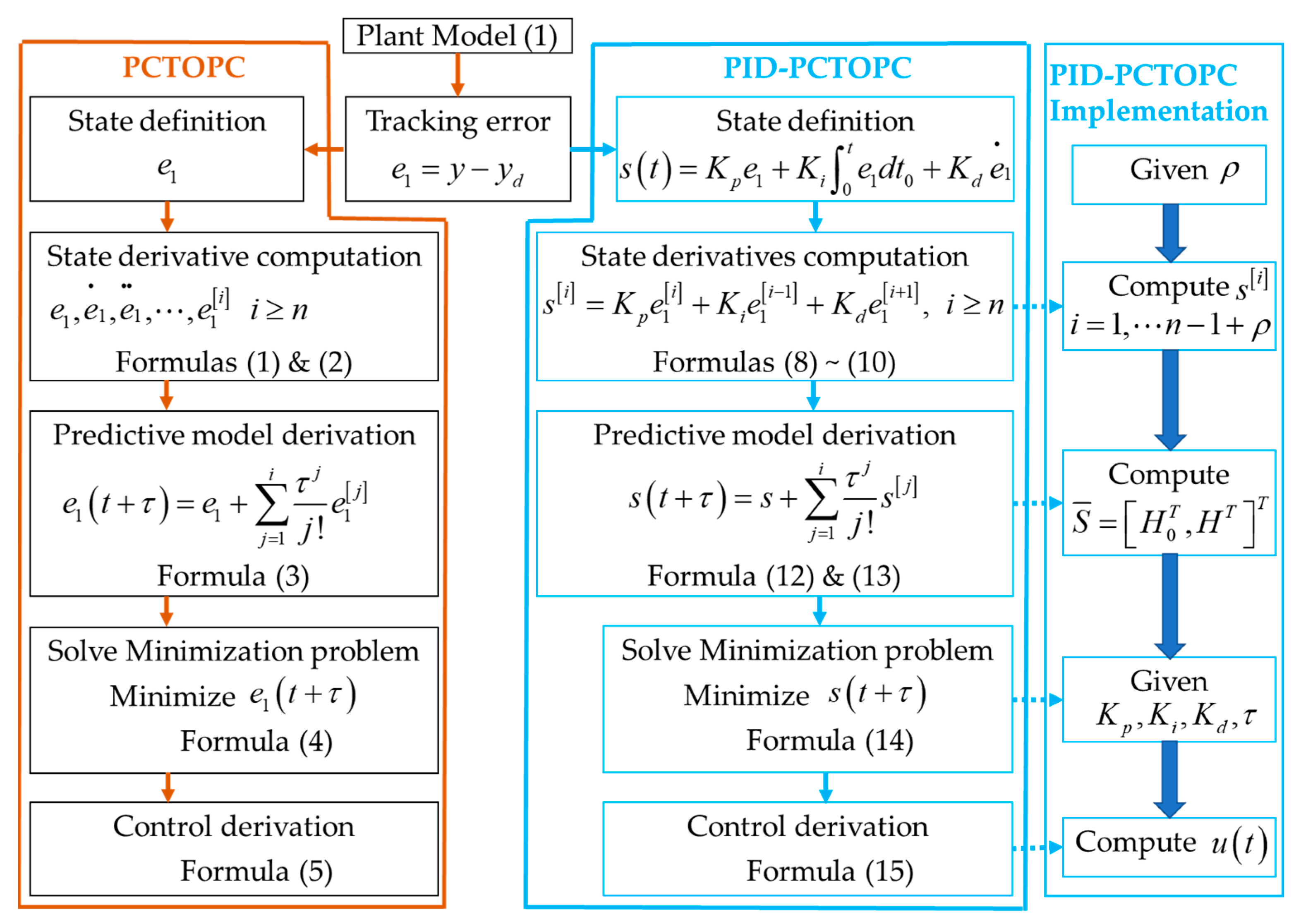
3.4. Connections and Comparisons between the PCTOPC and the PID-CTOPC

In this subsection, Figure 1 is applied to highlight both connections and differences between the PCTOPC and the proposed PID-CTOPC. Besides, flow chart for implementation of the PID-CTOPC is also illustrated in the figure.

4. Model Simulation Results

This section aims to demonstrate the effectiveness of the PID-CTOPC approach numerically through designing autopilots for a missile under external disturbances. Comparison with the PCTOPC and the Lu’s approach is carried out to highlight the superiorities of the PID-CTOPC. Lu’s approach can enable the closed-loop system better robustness than the one based upon the PCTOPC and has made many achievements [34,35,36,37,38,39,40,41,42,43,44,45]. Introduction of Lu’s approach targeting system (1) is given in Appendix A.

Longitudinal dynamics of a missile flying at Mach 3 and an altitude of 6096 m (20,000 ft) perturbed by disturbance is given by [19,40]:

$$\{\begin{array}{l}\stackrel{·}{\alpha }=\frac{0.7P_{0}S}{m{v}_s}{M}_a{C}_n\cos \alpha +q\\ \stackrel{·}{q}=\frac{0.7P_{0}S{d}_r}{I_y}{M}_a^2{C}_m\\ \stackrel{·}{{\delta }_1}={\delta }_2\\ \stackrel{·}{{\delta }_2}=-{\omega }_a^2{\delta }_1-2{\xi }_a{\omega }_a{\delta }_2+{\omega }_a^2{\delta }_c+d\left(t\right)\end{array}$$

(27)

where, $d\left(t\right)$ represents the unknown external disturbance. The force coefficient $C_n$ and the torque coefficient $C_m$ are given by:

$$\{\begin{array}{l}{C}_n=a_n{\alpha }^3{k}^3+b_n\alpha \left|\alpha \right|k^2+c_n\left(2-\frac{M_a}{3}\right)\alpha k+d_{n}k{\delta }_1\\ C_m=a_m{\alpha }^3{k}^3+b_m\alpha \left|\alpha \right|k^2+c_m\left(-7+\frac{8M_a}{3}\right)\alpha k+d_{m}k{\delta }_1\end{array}$$

(28)

where, $\alpha$, $q$, ${\delta }_1$, and ${\delta }_2$ are system states. $\alpha$ and $q$ represent the attack angle (rad) and the pitch rate (rad/s), respectively. Differential equations of ${\delta }_1$ and ${\delta }_2$ describe the actuator dynamics. ${\delta }_c$ represents the tail deflection (rad) as well as the control input, which ranges from −30 degree to 30 degree. The attack angle $\alpha$ is taken as the system output, which ranges from −20 degree to 20 degree. Values of the model parameters in Formulas (27) and (28) can be seen in [19,46].

Two simplifications in [19] are adopted. Firstly, $\cos \alpha \approx 1$. Secondly, since the control surface mainly generates rotational torque, thus, its contribution in the force equation $C_n$, namely, the term $d_{n}k{\delta }_1$, is ignored. Hence, in the controller design, ${\overline{C}}_n=a_n{\alpha }^3{k}^3+b_n\alpha \left|\alpha \right|k^2+c_n\left(2-\frac{M_a}{3}\right)\alpha k$ is used to replace $C_n$. In addition, to write the missile dynamics into the form in system, let $x={\left[x_1,x_2,x_3,x_4\right]}^T={\left[\alpha ,q,{\delta }_1,{\delta }_2\right]}^T$ and denote:

$$\{\begin{array}{l}{\left[f_1\left(x\right),f_2\left(x\right),f_3\left(x\right),f_4\left(x\right)\right]}^T={\left[\frac{0.7P_{0}S}{m{v}_s}{M}_a{\overline{C}}_n+q,\frac{0.7P_{0}S{d}_r}{I_y}{M}_a^2{C}_m,{\delta }_2,-{\omega }_a^2{\delta }_1-2{\xi }_a{\omega }_a{\delta }_2\right]}^T\\ {\left[g_1\left(x\right),g_2\left(x\right),g_3\left(x\right),g_4\left(x\right)\right]}^T={\left[0,0,0,{\omega }_a^2\right]}^T\end{array}$$

(29)

Next, to design the controller, the unknown external disturbance $d\left(t\right)$ is assumed to be zero. Then, in the simulation, $d\left(t\right)$ is considered. Differentiating the attack angle $\alpha$ four times yields:

$$\{\begin{array}{l}\stackrel{·}{\alpha }=f_1\left(x\right)\\ \stackrel{··}{\alpha }=\frac{\partial f_1\left(x\right)}{\partial x_1}{f}_1\left(x\right)+f_2\left(x\right)\\ {\alpha }^{\left[3\right]}=\left[\frac{{\partial }^2{f}_1\left(x\right)}{\partial x_1^2}{f}_1\left(x\right)+{\left(\frac{\partial f_1\left(x\right)}{\partial x_1}\right)}^2+\frac{\partial f_2\left(x\right)}{\partial x_1}\right]f_1\left(x\right)+\frac{\partial f_1\left(x\right)}{\partial x_1}{f}_2\left(x\right)+\frac{\partial f_2\left(x\right)}{\partial x_3}{f}_3\left(x\right)\\ {\alpha }^{\left[4\right]}={\rho }_1\left(x\right)\cdot f_1\left(x\right)+{\rho }_2\left(x\right)\cdot f_2\left(x\right)+\frac{\partial f_1\left(x\right)}{\partial x_1}\cdot \frac{\partial f_2\left(x\right)}{\partial x_3}{f}_3\left(x\right)+\frac{\partial f_2\left(x\right)}{\partial x_3}{f}_4\left(x\right)+\frac{\partial f_2\left(x\right)}{\partial x_3}{g}_4\left(x\right)\cdot u\end{array}$$

(30)

where, the nonlinear terms ${\rho }_1\left(x\right)$ and ${\rho }_2\left(x\right)$ are given by:

$$\{\begin{array}{l}{\rho }_1\left(x\right)=\frac{\partial f_1^3\left(x\right)}{\partial x_1^3}{f}_1^2\left(x\right)+\frac{\partial f_1^2\left(x\right)}{\partial x_1^2}\left[4f_1\left(x\right)\frac{\partial f_1\left(x\right)}{\partial x_1}+f_1\left(x\right)+f_2\left(x\right)\right]+2\frac{\partial f_1\left(x\right)}{\partial x_1}\cdot \frac{\partial f_2\left(x\right)}{\partial x_1}+{\left[\frac{\partial f_1\left(x\right)}{\partial x_1}\right]}^3\\ {\rho }_2\left(x\right)=2f_1\left(x\right)\frac{\partial f_1^2\left(x\right)}{\partial x_1^2}+{\left[\frac{\partial f_1\left(x\right)}{\partial x_1}\right]}^2+\frac{\partial f_2\left(x\right)}{\partial x_1}\end{array}$$

(31)

It can be verified that $m\left(x\right)\ne 0$. Therefore, the system dimension is $n=4$.

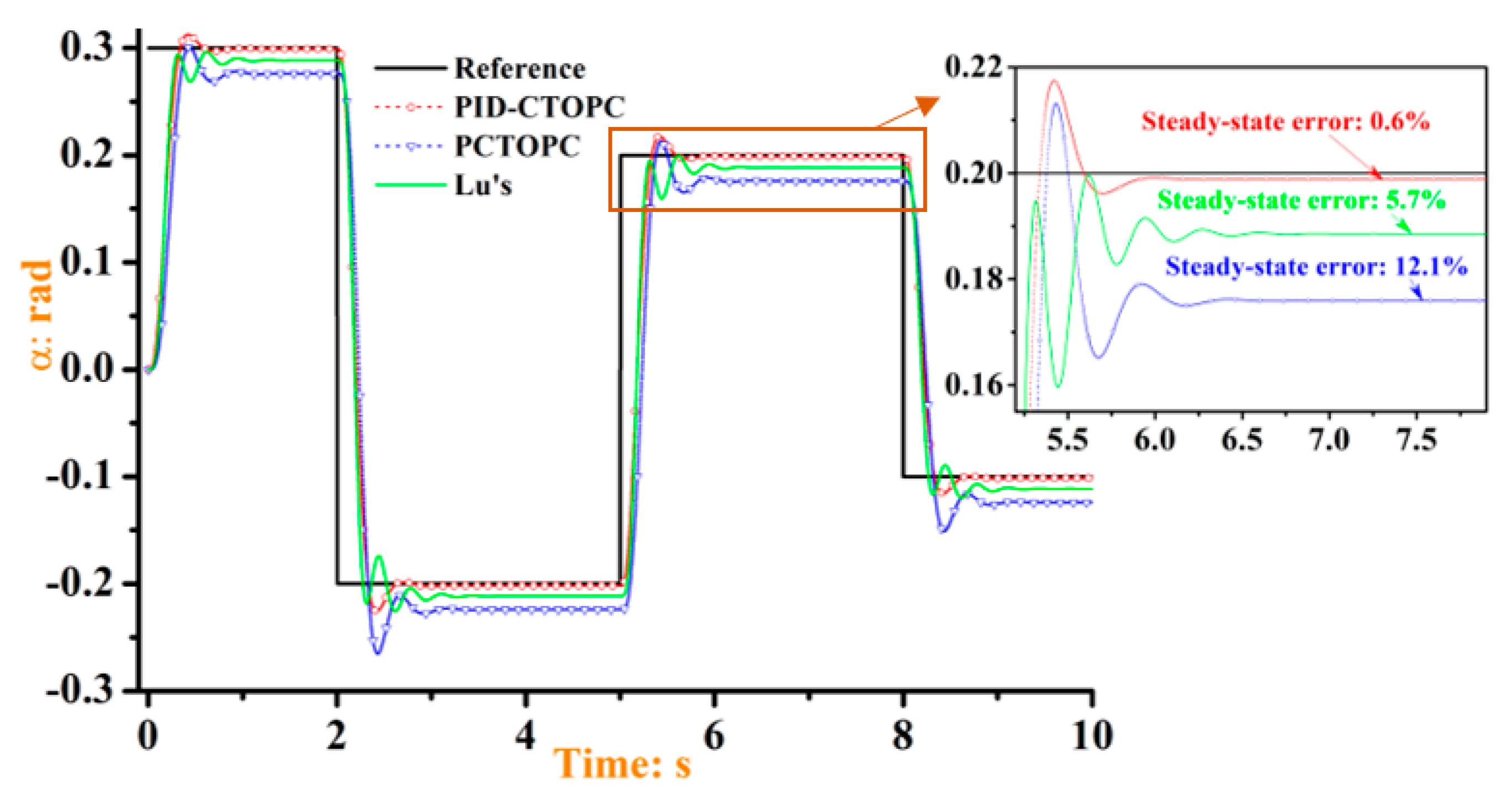
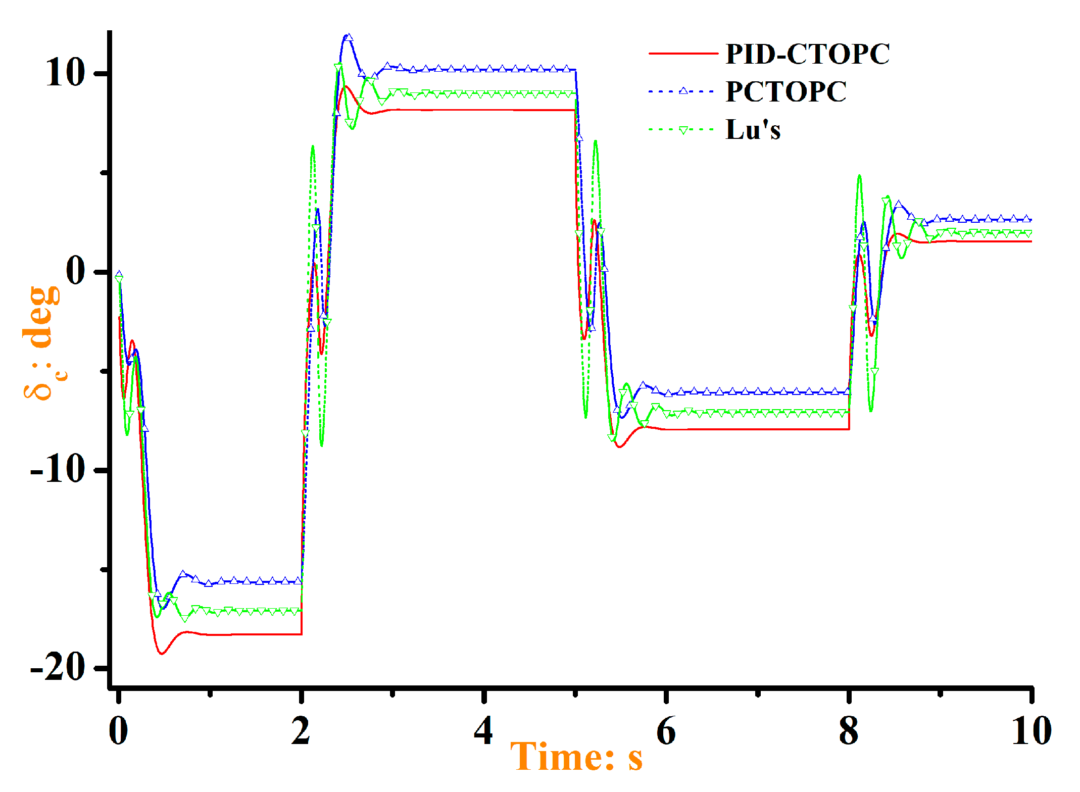
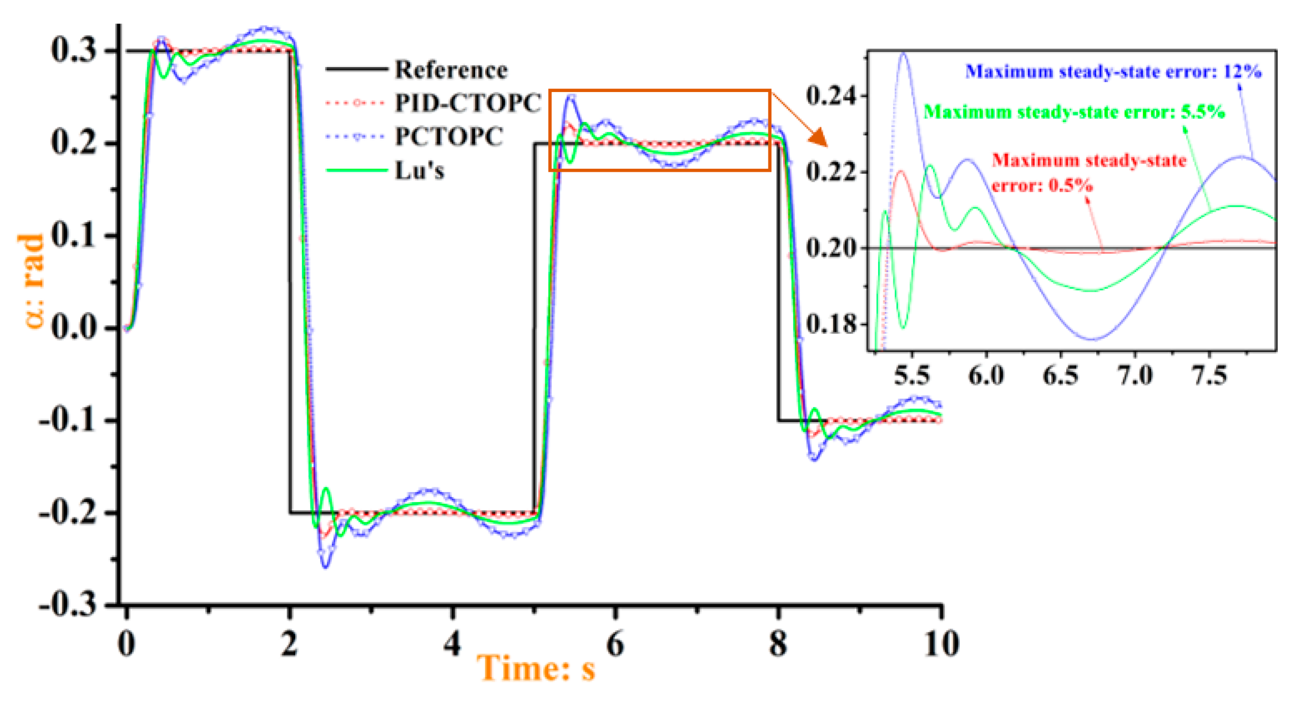
4.1. Case Study 1: Superioities Validation

In this subsection, two groups of simulations are carried out in MATLAB/Simulink with the simulation time 10 s and the sampling interval 0.002 s. The prescribed reference (unit: rad) is given by: ${\alpha }_d\left(t\right)=0.3$ when $t\le 2$, ${\alpha }_d\left(t\right)=-0.2$ when $2\le t\le 5$, ${\alpha }_d\left(t\right)=0.2$ when $5\le t\le 8$, and ${\alpha }_d\left(t\right)=-0.1$ when $8\le t\le 10$. Then, derivatives of ${\alpha }_d\left(t\right)$ are given by: ${\stackrel{·}{\alpha }}_d\left(t\right)={\stackrel{··}{\alpha }}_d\left(t\right)={\alpha }_d^{\left[3\right]}\left(t\right)={\alpha }_d^{\left[4\right]}\left(t\right)=0$. Reference values of the controller parameters are given in

Table 1. Values of controller parameters.

Approach Name	Parameter Value
PID-CTOPC	$t_M=0.5$, $\rho =2$, $K_p=10$, $K_i=0.1$, $K_d=0.05$
PCTOPC	$t_C=0.5$, $\sigma =2$
Lu’s	$t_L=0.08$, $Q_1=100$, $Q_2=0.2$, $Q_3=Q_4=0$

.

Controller parameters of the three approaches are given based on the performance index that the autopilot system has almost the same response time. In the first group of simulation, the system is affected by constant disturbance $d\left(t\right)=5$. Then, in the second group, time-varying disturbance $d\left(t\right)=5\sin \left(\pi t\right)$ is added to the system. The two types of disturbances are only used to show the superiorities of the modified approach, which may have differences with the real scenarios.

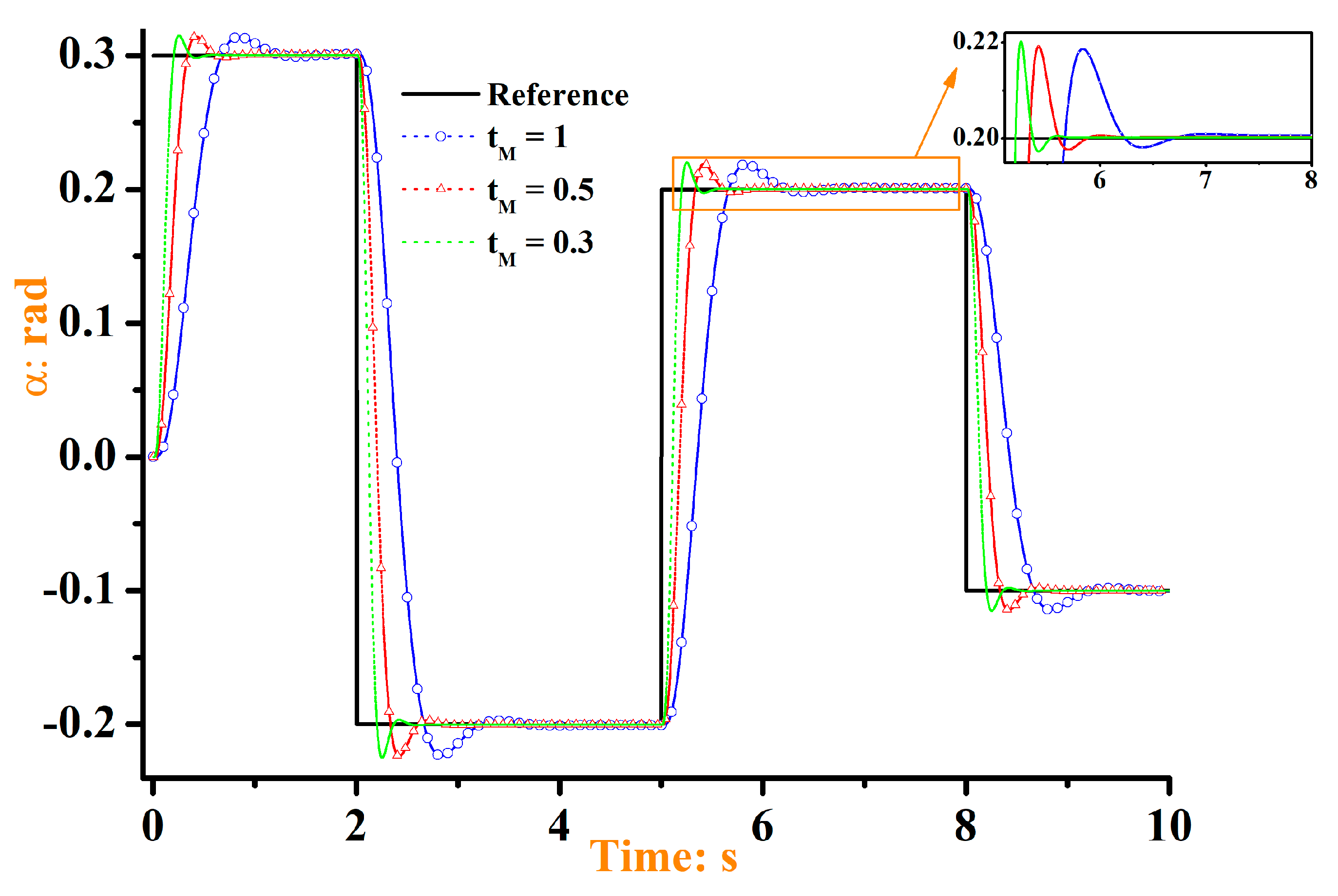
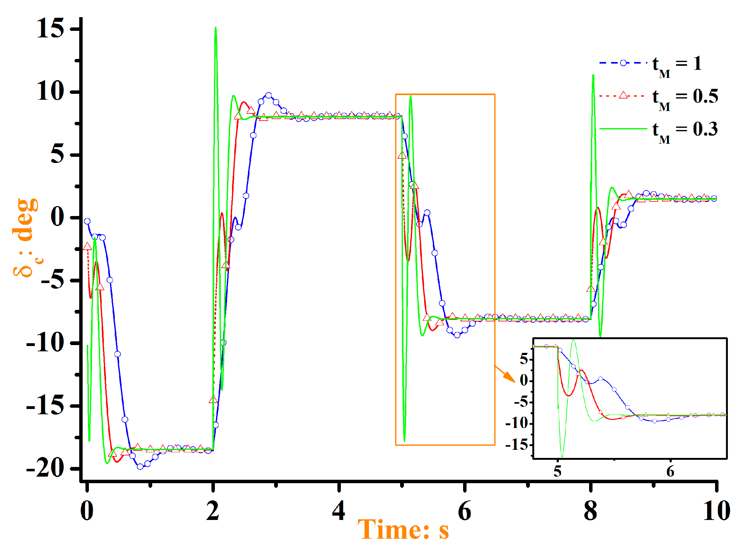
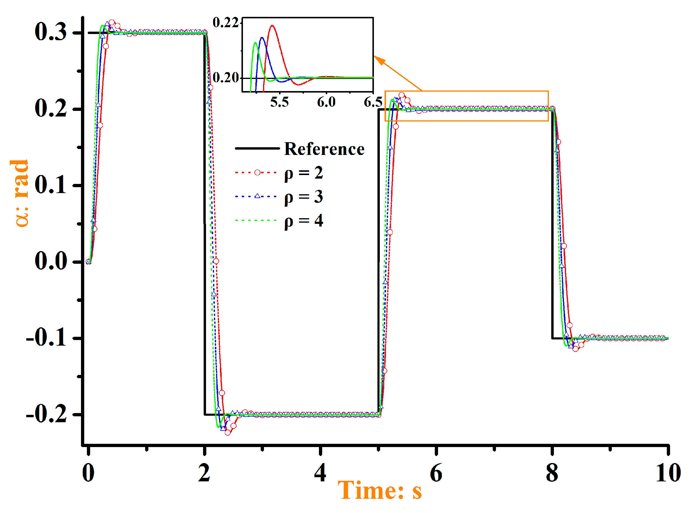
4.2. Case Study 2: Control Parameter Selection Validation

In this subsection, since tuning principles of $K_p$, $K_i$, and $K_d$ are the same with the conventional PID controllers, which has been pointed out before, thus, influences on the PID-CTOPC-based closed-loop performance from the control parameters $t_M$ and $\rho$ are mainly discussed. Values of $\rho$, $K_p$, $K_i$, and $K_d$ are the same with the ones shown in Table 1. In addition, to clearly show the influences, disturbances are not considered in next.

First, closed-loop performance based upon difference values of the predictive period, namely, $t_M=1$, $t_M=0.5$, and $t_M=0.3$ is illustrated.

Second, closed-loop performance based upon difference values of the control order, namely, $\rho =2$, $\rho =3$, and $\rho =4$ is illustrated.

5. Discussion

Contrast results for Case study 1 are given by Figure 2:

It can be seen from Figure 2, Figure 3, Figure 4 and Figure 5 that, the PID-CTOPC approach is obviously superior to the two representative predictive approaches under the constant and time-varying external disturbances. For one thing, due to the consideration of the accumulative tracking error in the new error state, the proposed PID-CTOPC approach-based closed-loop system has smaller state-steady error than the one based on the PCTOPC and the Lu’s approach, as shown in Figure 2 and Figure 4. For another thing, using appropriate linear combination of the current, accumulative, and derivative tracking errors and minimizing the three errors simultaneously in the optimization problem are beneficial to reduce input fluctuations for the proposed approach compared with the PCTOPC and Lu’s approach, which is also illustrated in Figure 3 and Figure 5.

It can be seen from Figure 6 and Figure 7 that a large value of the predictive period corresponds to fast system output response speed, while it would bring the closed-loop system obvious negative effects in which fluctuation and surging of the system input become serious in dealing with sudden changes. Thus, to derive satisfied control performance, one should balance the response speed and the input fluctuation by adjusting the value of the predictive period.

Figure 8 and Figure 9 clearly illustrate that, though increasing the value of the control order would lead to small response time of the closed-loop system, frequent fluctuation and surging of the system input would occur when the sudden changes are encountered. Thus, tuning the value of the control order is another way to weigh the response speed and the input fluctuation for the closed-loop system.

6. Conclusions

This paper improves the output performance for a class of high-order nonlinear systems under unknown constant and time-varying external disturbances by modifying the PCTOPC approach. The main conclusions are drawn as:

• A new system error state with PID structure is presented such that the current, the accumulative, and the derivative tracking errors are all considered and then minimized in the optimization problem simultaneously.
• Due to the minimization of the accumulative and derivative tracking errors in the proposed optimal predictive controller, robustness of the closed-loop system against the constant and the time-varying disturbances is significantly enhanced and the system input fluctuations are also degraded compared with the system using the controllers based upon the PCTOPC and the Lu’s approaches.
• Though the proposed PID-CTOPC have achieved satisfactory control performance, there are some further studies that can be expected in the future. First, the proposed approach is expected to be validated experimentally. Second, the control parameters are required to be adjusted adaptively by using tracking errors.

References

1. Dobroskok, N.A.; Vtorov, V.B. Robust Pole Assignment in a Problem of State Observer-based Modal Control. In Proceedings of the 2021 IV International Conference on Control in Technical Systems (CTS), Saint Petersburg, Russia, 21–23 September 2021; pp. 30–33. [Google Scholar]
2. Hideaki, H.; Kenshiro, K.; Shu, Y. Simple Design Method of Two-Degree-of-Freedom PID Position Controller Based on Pole-Zero-Assignment for Linear Servo Motors. In Proceedings of the 2020 23rd International Conference on Electrical Machines and Systems (ICEMS), Hamamatsu, Japan, 24–27 November 2020; pp. 1800–1805. [Google Scholar]
3. Ahmet, E.; Aziz, K. Feedback linearization control of a quadrotor. In Proceedings of the 2021 5th International Symposium on Multidisciplinary Studies and Innovative Technologies (ISMSIT), Ankara, Turkey, 21–23 October 2021; pp. 287–290. [Google Scholar]
4. Adamiak, K. Time-Variant Discrete-Time Sliding Mode Control. In Proceedings of the 2021 22nd International Carpathian Control Conference (ICCC), Velké Karlovice, Czech Republic, 31 May–1 June 2021; pp. 1–5. [Google Scholar]
5. Adamu, A.; Sirin, A. Adaptive Cruise Control: A Model Reference Adaptive Control Approach. In Proceedings of the 2020 24th International Conference on System Theory, Control and Computing (ICSTCC), Sinaia, Romania, 8–10 October 2020; pp. 904–908. [Google Scholar]
6. Tan, X.; Wang, H.M.; Peng, W.W.; Liang, N.; Zhang, W. Finite-Time Disturbance Attenuation Tracking Control of Flexible-Joint Robots Based on CTSMC. In Proceedings of the 2021 40th Chinese Control Conference (CCC), Shanghai, China, 26–28 July 2021; pp. 604–609. [Google Scholar]
7. Chen, Y.Y.; Wang, Y.; Dong, Q.; Zhu, G.M.; Feng, J.J.; Xiao, F.Y. Robust adaptive back-stepping control for nonlinear systems with unknown backlash-like hysteresis. In Proceedings of the 2021 IEEE International Conference on Mechatronics and Automation (ICMA), Takamatsu, Japan, 8–11 August 2021; pp. 554–559. [Google Scholar]
8. Chen, W.H.; Balance, D.J.; Gawthrop, P.J. Optimal control of nonlinear systems: A predictive control approach. Automatica 2003, 39, 633–641. [Google Scholar] [CrossRef] [Green Version]
9. Chen, J.L.; Sun, L.; Sun, G.; Li, Y.Y.; Zhu, B. Generalized predictive tracking control of spacecraft attitude based on hyperbolic tangent extended state observer. Adv. Space Res. 2020, 66, 335–344. [Google Scholar] [CrossRef]
10. Sun, G.; Chen, J.L.; Zhu, B. Generalized predictive control for spacecraft attitude based on adaptive fuzzy estimator. J. Aerosp. Eng. 2017, 30, 04017024. [Google Scholar] [CrossRef]
11. Liu, X.D.; Zhang, C.H.; Zhang, K.L. Nonlinear predictive high order sliding mode control for permanent magnet synchronous motor drive system. J. Math. Comput. Sci. 2016, 16, 402–411. [Google Scholar] [CrossRef] [Green Version]
12. Xu, Z.A.; Shi, Q.; Wei, Y.J.; Wang, M.W.; He, Z.J.; He, L. A Generalized Predictive Control Approach for Angle Tracking of Steer-by-Wire System. In Proceedings of the 60th Annual Conference of the Society of Instrument and Control Engineers of Japan (SICE), Tokyo, Japan, 8–10 September 2021; pp. 272–275. [Google Scholar]
13. Yang, J.; Cui, H.Y.; Li, S.H.; Zolotas, A. Optimized active disturbance rejection control for DC-DC buck converters with uncertainties using a reduced-order GPI observer. IEEE Trans. Circuits Syst. I 2018, 65, 832–841. [Google Scholar] [CrossRef] [Green Version]
14. Errouissi, R.; Al-Durra, A.; Muyeen, S.M. A robust continuous-time MPC of a dc-dc boost converter interfaced with a grid-connected photovoltaic system. IEEE J. Photovolt. 2016, 6, 1619–1629. [Google Scholar] [CrossRef] [Green Version]
15. Cui, J.L.; Chen, Z.; Shen, J.W.; Shen, S.Q.; Liu, Y.G. Robust Cascaded Nonlinear Generalized Predictive Control with Sliding Mode Disturbance Observer for Permanent Magnet Synchronous Hub Motor. In Proceedings of the 2020 4th CAA International Conference on Vehicular Control and Intelligence (CVCI), Hangzhou, China, 8–2 December 2020; pp. 276–281. [Google Scholar]
16. Merabet, A.; Labib, L.; Ghias, A.M.Y.M. Robust model predictive control for photovoltaic inverter system with grid fault ride-through capability. IEEE Trans. Smart Grid 2018, 9, 5699–5709. [Google Scholar] [CrossRef]
17. Errouissi, R.; Muyeen, S.M.; Al-Durra, A.; Leng, S.Y. Experimental validation of a robust continuous nonlinear model predictive control based grid-interlinked photovoltaic inverter. IEEE Trans. Ind. Electron. 2016, 63, 4495–4505. [Google Scholar] [CrossRef] [Green Version]
18. Aissou, R.; Rekioua, T.; Rekioua, D.; Tounzi, A. Application of nonlinear predictive control for charging the battery using wind energy with permanent magnet synchronous generator. Int. J. Hydrogen Energy 2016, 41, 20964–20973. [Google Scholar] [CrossRef]
19. Ouari, K.; Rekioua, T.; Ouhrouche, M. Real time simulation of nonlinear generalized predictive control for wind energy conversion system with nonlinear observer. ISA Trans. 2014, 53, 76–84. [Google Scholar] [CrossRef]
20. Gouta, H.; SaÏd, S.H.; Barhoumi, N.; M’Sahli, F. Generalized predictive control for a coupled four tank MIMO system using a continuous-discrete time observer. ISA Trans. 2017, 67, 280–292. [Google Scholar] [CrossRef] [PubMed]
21. Gouta, H.; SaÏd, S.H.; Barhoumi, N.; M’Sahli, F. Model-based predictive and backstepping controllers for a state coupled four-tank system with bounded control inputs: A comparative study. J. Franklin Inst. 2015, 352, 4864–4889. [Google Scholar] [CrossRef]
22. Wang, D.Z.; Zhao, D.X.; Gong, M.D.; Yang, B. Nonlinear Predictive Sliding Mode Control for Active Suspension System. Shock Vib. 2018, 2018, 8194305. [Google Scholar] [CrossRef] [Green Version]
23. Jing, S.; Errouissi, R.; Al-Durra, A.; Boiko, I. Stabilization of artificial gas-lift process using nonlinear predictive generalized minimum variance control. In Proceedings of the 2016 American control conference (ACC), Boston, MA, USA, 6–8 July 2016; pp. 4169–4174. [Google Scholar]
24. Krid, M.; Benamar, F.; Lenain, R. A new explicit dynamic path tracking controller using generalized predictive control. Int. J. Control Autom. Syst. 2016, 15, 303–314. [Google Scholar] [CrossRef]
25. Filho, J.M.M.; Lucet, E.; Filliat, D. Real-Time Distributed Receding Horizon Motion Planning and Control for Mobile Multi-Robot Dynamic Systems. In Proceedings of the International Conference on Robotics and Automation (ICRA), Singapore, 29 May–1 June 2017; pp. 657–663. [Google Scholar]
26. Khoukhi, B.; Tadjine, M.; Boucherit, M.S. Nonlinear continuous-time generalized predictive control of solar power plant. Int. J. Simul. Multidiscip. Des. Optim. 2015, 6, A3. [Google Scholar] [CrossRef] [Green Version]
27. Invernizzi, D.; Panza, S.; Lovera, M. Robust Tuning of Geometric Attitude Controllers for Multirotor Unmanned Aerial Vehicles. J. Guid. Control Dyn. 2020, 43, 1332–1343. [Google Scholar] [CrossRef]
28. Ghiglino, P.; Forshaw, J.L.; Lappas, V.J. Online evolutionary swarm algorithm for self-tuning unmanned flight control laws. J. Guid. Control Dyn. 2015, 38, 772–782. [Google Scholar] [CrossRef]
29. Yoo, C.H. Active control of aeroelastic vibrations for electromechanical missile fin actuation systems. J. Guid. Control Dyn. 2017, 40, 3296–3303. [Google Scholar] [CrossRef]
30. Zhang, R.D.; Wu, S.; Gao, F.R. Improved pi controller based on predictive functional control for liquid level regulation in a coke fractionation tower. J. Process Control 2014, 24, 125–132. [Google Scholar] [CrossRef]
31. Yu, H.; Guan, Z.; Chen, T.W.; Yamamoto, T. Design of data-driven PID controllers with adaptive updating rules. Automatica 2020, 121, 109185. [Google Scholar] [CrossRef]
32. Lu, P. Nonlinear Predictive Controllers for Continuous Systems. J. Guid. Control Dyn. 1994, 17, 553–560. [Google Scholar] [CrossRef]
33. Lu, P. Optimal Predictive Control of Continuous Nonlinear Systems. Int. J. Control 1995, 62, 633–649. [Google Scholar] [CrossRef]
34. Lu, P. Constrained Tracking Control of Nonlinear Systems. Syst. Control Lett. 1996, 27, 305–314. [Google Scholar] [CrossRef]
35. Singh, S.N.; Steinberg, M.; DiGirolamo, R.D. Nonlinear Predictive Control of Feedback Linearizable Systems and Flight Control System Design. J. Guid. Control Dyn. 1995, 18, 1023–1028. [Google Scholar] [CrossRef]
36. Lu, P.; Pierson, B.L. Aircraft Terrain Following Based on a Nonlinear Continuous Predictive Control Approach. J. Guid. Control Dyn. 1995, 18, 817–823. [Google Scholar] [CrossRef]
37. Lee, I.H.; Bang, H. A Cooperative Line-of-Sight Guidance Law for a Three-Dimensional Phantom Track Generation using Unmanned Aerial Vehicles. Proc. Inst. Mech. Eng. Part G J. Aerosp. Eng. 2012, 227, 897–915. [Google Scholar] [CrossRef]
38. Lu, P. Entry Guidance and Trajectory Control for Reusable Launch Vehicle. J. Guid. Control Dyn. 1997, 20, 143–149. [Google Scholar] [CrossRef]
39. Lu, P.; Hanson, J.M. Entry Guidance for the X-33 Vehicle. J. Spacecr. Rocket. 1998, 35, 342–349. [Google Scholar] [CrossRef]
40. Brinda, V.; Dasgupta, S. Guidance Law for an Air-Breathing Launch Vehicle Using Predictive Control Concept. J. Guid. Control Dyn. 2006, 29, 1460–1463. [Google Scholar] [CrossRef]
41. Khan, M.A.; Lu, P. New Techniques for Nonlinear Control of Aircraft. J. Guid. Control Dyn. 1994, 17, 1055–1060. [Google Scholar] [CrossRef]
42. Crassidis, J.L.; Markley, F.L.; Anthony, T.C.; Andrews, S.F. Nonlinear Predictive Control of Spacecraft. J. Guid. Control Dyn. 1997, 20, 1096–1103. [Google Scholar] [CrossRef]
43. Bang, H.; Oh, C.S. Predictive Control for the Attitude Maneuver of a Flexible Spacecraft. Aerosp. Sci. Technol. 2004, 8, 443–452. [Google Scholar] [CrossRef]
44. Panchal, B.; Kolhe, J.P.; Talole, S.E. Robust predictive control of a class of nonlinear systems. J. Guid. Control Dyn. 2014, 37, 1437–1445. [Google Scholar] [CrossRef]
45. Panchal, B.; Mate, N.; Talole, S.E. Continuous-time predictive control-based integrated guidance and control. J. Guid. Control Dyn. 2017, 40, 1579–1595. [Google Scholar] [CrossRef]
46. Fromion, V.; Scorletti, G.; Ferreres, G. Nonlinear performance of a PI controlled missile: An explanation. Int. J. Robust Nonlinear Control 2015, 9, 485–518. [Google Scholar] [CrossRef]
Figure 1. Connections and comparisons between the PCTOPC and the PID-CTOPC.
Applsci 12 05446 g001
Figure 2. Group 1 with constant disturbance: Attack angle α .
Applsci 12 05446 g002
Figure 3. Group 1 with constant disturbance: Tail deflection δ c .
Applsci 12 05446 g003
Figure 4. Group 2 with time-varying disturbance: Attack angle α .
Applsci 12 05446 g004
Figure 5. Group 2 with time-varying disturbance: Tail deflection δ c .
Applsci 12 05446 g005
Figure 6. Validation with different predictive period t M : Attack angle α .
Applsci 12 05446 g006
Figure 7. Validation with different predictive period t M : Tail deflection δ c .
Applsci 12 05446 g007
Figure 8. Validation with different control order ρ : Attack angle α .
Applsci 12 05446 g008
Figure 9. Validation with different control order ρ : Tail deflection δ c .
Applsci 12 05446 g009