Article

Multi-Label Classification and Explanation Methods for Students’ Learning Style Prediction and Interpretation

by
Daiva Goštautaitė
* and
Leonidas Sakalauskas
Department of Information Technologies, Vilnius Gediminas Technical University, 10223 Vilnius, Lithuania
*
Author to whom correspondence should be addressed.
Appl. Sci. 2022, 12(11), 5396; https://doi.org/10.3390/app12115396
Submission received: 22 April 2022 / Revised: 21 May 2022 / Accepted: 24 May 2022 / Published: 26 May 2022

Abstract

:

Featured Application

As students are usually characterized by more than one learning style, multi-label classification methods may be applied for the diagnosis of a composite students’ learning style, based on each learner’s activities in the virtual learning environment. For data sets with weakly correlated learning activities, Shapley values present the explanations for the predicted student’s multi-label learning style. In this way, the model assists teachers in better understanding the cognitive traits of the learners in terms of learning activities, enabling teachers to prepare the relevant learning objects for the personalization of virtual learning environments.

Abstract

The current paper attempts to describe the methodology guiding researchers on how to use a combination of machine learning methods and cognitive-behavioral approaches to realize the automatic prediction of a learner’s preferences for the various types of learning objects and learning activities that may be offered in an adaptive learning environment. Generative as well as discriminative machine learning methods may be applied to the classification of students’ learning styles, based on the student’s historical activities in the e-learning process. This paper focuses on the discriminative models that try to learn which input activities of the student(s) will correlate with a particular learning style, discriminating among the inputs. This paper also investigates several interpretability approaches that may be applicable for the multi-label models trained on non-correlated and partially correlated data. The investigated methods and approaches are combined in a consistent procedure that can be used in practical learning personalization.

1. Introduction

The personalization of the virtual learning environment (VLE) reflects the ways in which learning processes may be controlled so that each environment is optimally attractive to the learner. This includes personalized navigation, a personalized recommendation engine, personal instructors, personalized learning paths, fragment sorting and content adaptation as a means to customize learning objects for constrained environments, and student knowledge diagnosis as a task in realizing personalized education, among others [1,2,3,4,5,6,7,8,9]. VLE constraints may be dictated by both personal preferences and the learning style of the learner [10]. In general, “learning styles” refer to a range of theories that aim to account for differences in individual learning methods. Many theories share the proposition that humans can be classified according to their “style” of learning but differ in how the proposed styles should be defined, categorized, and assessed [11].
The learning style of the learner can be automatically determined by the learner’s activities in a virtual learning environment [12]. Automatic identification of the learning style of the learner(s) employs user modeling, which may be divided into static or dynamic modeling, via stereotypes and highly adaptive user models [13].
In our previous papers, we investigated the exemplar-based methods that are sometimes applied to automatic learning-style diagnostics [14,15]. For example, the Bayesian case model (BCM) is a generative format that uses unsupervised learning methods and may predict the proportions of learning-style clusters for each student. Probabilistic models, in general, try to use the Bayes formula or mixture models in a multi-label scenario [16]. In addition, BCM offers explanations for each learning-style cluster, using prototypes and important features. In unsupervised learning, only input data is provided to the model. Conversely, in supervised learning, input data is provided to the model, along with the output data. The goal of supervised learning is to train the model so that it can predict the output when it is given new data. The supervised user (learner) model classifies students into their particular classes according to their learning style (for example, visual, kinesthetic, aural, social, solitary, verbal, or logical) and/or assigns multiple learning-style labels to the learner. Multi-label classification allows the model to classify data sets with more than one target variable [17]. When making predictions, a given input may belong to more than one label.
The task of determining the learning style of a student (or a group of students) may be treated as a multi-label classification task. Formally, multi-label classification is the problem of finding a model that maps input x to binary vector y (assigning a value of 0 or 1 for each element (label) in y). In the case of students’ learning styles, prediction labels might be taken from the widely adopted Felder–Silverman model [10], wherein learning styles are a balance between pairs of extremes, such as Active/Reflective, Sensing/Intuitive, Verbal/Visual, and Sequential/Global. Each student or a group of students may be assigned a set of these labels by the model, and some of the labels are more typical for a particular student (or group of students) than others. Therefore, for each label, the model should predict the probability that the student (or group of students) is characterized by the label(s). The model might be trained on the data set, manually labeled by experts, that stores students’ activities in the VLE. The values of the data features primarily store the number of times that a particular learning activity was selected by a student or for how long it was used by the student in question.
Therefore, the aim of this research is to identify multi-label classification methods that are suitable for students’ learning-style detection, as well as the interpretation methods that can explain the classification results. These methods must be combined into a coherent and logical methodology, providing the solution to learning-style identification. Later learning style(s) may be used for personalization of the VLE.
Of the many papers on learning personalization, not a single author has addressed the lack of experimental work in the area of automatic student learning-style prediction and the personalization of learning environments. Trying to fill this gap, we conducted experiments for determining students’ learning styles, using supervised machine learning methods. Students’ learning-style identification is related to multi-learning problems—multiclass, multi-label, or multi-output classification methods may be applied to solve them, depending on the specific need [18]. Multi-label classification is most likely to be used in practical applications since a student is very rarely characterized by a single learning style—usually, several dominant learning styles interact for each learner. Therefore, this paper describes our experiments with multi-label classification solutions.
Another learning-style modeling aspect that requires consideration is interpretability. Interpretability is about the extent to which a particular cause and effect can be observed within a system. It is not enough to have the probability values of a student’s learning style—teachers, students, and other stakeholders may want or need to understand the reasoning behind the predictions and decisions made by the model. In this way, for example, teachers could prepare learning objects of certain types (video, text, or audio) or develop learning content that is appropriate to the group of students, who may be characterized by a particular learning style. In this context, it is also important to understand the difference between interpretability and explainability. Explainability is the extent to which the internal mechanics of a deep learning system can be explained in human terms. In turn, interpretability is the capacity to consistently explain (interpret) model’s result without trying to know the reasons behind the scenes. The model agnostic SHAP (Shapley additive explanations) method is proposed to explain NN’s individual predictions for those cases when the input data features are not correlated or weakly correlated.
When proposing multi-label classification methods for students’ learning-style detection, more sophisticated practical cases were also taken into account: classifier chains [19] and other methods for correlating labels, asymmetric Shapley values for incorporating causal knowledge into model explainability, etc.
Besides the above-mentioned points, the experimental work described in this paper deals with the input data preprocessing techniques (data scaling, under/oversampling in the case of imbalanced data sets, imputation strategies in the case of missing input data values, etc.) and the methods used to prevent the model from overfitting (for example, the dropout approach or regularization techniques).
This research and the pilot experimental results led to our creating a set of procedures and methods for identifying a student’s learning style and personalizing the virtual learning environment accordingly.
The rest of the paper is organized as follows: firstly, the existing categories of multi-label approaches that may be applied in students’ learning-style classification are listed and briefly outlined; secondly, the model agnostic SHAP method that we propose for model interpretation is introduced. Then, the results of our experiments with multi-label approaches are described in Section 3. After an exploratory analysis of the training data set, we describe the experiments performed with the OneVsRest multi-label classifiers that use various base estimators (the problem transformation approach); based on the results of these experiments, the generalization quality of the classifiers is then compared, using such performance metrics as the Hamming loss, precision, recall, and the F1 score. Then, we move to algorithm adaptation methods and describe the experiment that was performed with a neural network for multi-label student learning-style prediction. After this, we present the results of our experimentation with Shapley values, which might be used to explain the neural network model. Then, the procedure describing how to select methods for multi-label students’ learning-style detection is proposed as the result of these experiments. Finally, conclusions are drawn, and suggestions for future work are mentioned in Section 5.
The main contribution of this article is a developed mechanism that can help other researchers to select the appropriate machine learning methods for student learning-style prediction and interpretation.

2. Methods

2.1. Systematic Review of the Literature

In the literature, not a single attempt was made to apply rule-based, statistical, and machine-learning methods for automatic student learning-style prediction. The authors of [20] mention existing Bayesian networks, the hidden Markov model, decision trees, NB tree classification, reinforcement learning, and other algorithms, and describe their experimentation with artificial neural networks, genetic algorithms, the ant colony system, and particle swarm optimization algorithms, using the Felder–Silverman learning style model to describe learning-style dimensions. Based on the results of these experiments, the authors concluded that different approaches perform best in different learning-style dimensions, but all the tested models outperformed the existing approaches.
Experiments with deep neural networks for learning-style prediction are presented in one study [2]. The authors selected an optimal neural network of two hidden layers for student learning-style prediction. For training the model, 100 samples were used. The Felder–Silverman learning-style dimensions were predicted as well. The authors also applied principal components analysis (PCA) to investigate “whether targets for each dimension might be explained by some descriptor (time and count)” [21]. The authors also presented NN performance metrics, including a detection rate that was between 0.2 and 0.5, depending on the dimension.
A comprehensive comparative study of multi-label classification (MLC) methods is presented by the authors of [16]—they evaluate 26 methods with 42 benchmark data sets, using 20 evaluation measures. The study includes both problem transformation and algorithm adaptation methods. The former group of methods decomposes the MLC problem into simpler problems that are addressed with standard machine-learning methods; the latter group of methods addresses the MLC problem in a holistic manner—it trains a model for predicting all labels simultaneously [16]. The authors selected the 8 best-performing methods: RFDTBR, AdaBoost.MH, ECCJ48, TREMLC, PSt, and EBRJ48 in terms of problem transformation, with RFPCT and BPNN as the algorithm adaptation methods [16]. The authors state that MLC methods have weaknesses as well as strengths, depending on what metrics are used for the evaluation. RFPCT, RFDTBR, EBRJ48, AdaBoost.MH and ECCJ48 were distinguished as the best-performing methods, considering all 18 evaluation measures.
The authors of [1] developed a learning agent for classifying students’ learning styles using an artificial neural network. Due to the lack of homogenous data, the data set was generated by stimulating students’ learning behavior, based on the five inputs.
Despite the fact that a plethora of papers exists about multiclass and multilabel classification (for example, [22,23,24,25]), not many experimental works applying problem transformation approaches to multi-label classification for student learning-style prediction have been published. For example, the authors of [26] present a summary of works in the automatic detection of learning styles and do not mention problem transformation approaches for multi-label classification at all. According to their research, decision tree, random forest, k-nearest neighbor and other classifiers achieve 74–90% accuracy for various learning style dimensions.
Many other student learning-style classification applications target mainly problem adaptation rather than problem transformation approaches.

2.2. Supervised Learning Algorithms for Classification

Theoretically, four types of classification tasks exist:
  • Binary classification;
  • Multi-class classification;
  • Multi-label classification;
  • Imbalanced classification (this uses such techniques as: random oversampling/under-sampling; SMOTE oversampling; examples of algorithms, such as cost-sensitive logistic regression and cost-sensitive decision trees).
Generally, all types of classification tasks may need to be addressed when practically classifying students’ learning styles. Moreover, there are various multi-class classification strategies and methods that solve such tasks: one vs. rest; one vs. one; output code-based strategy. Each of these may be applied to student learning-style diagnosis, depending on the specific need. The existing categories of multi-label approaches that may be applied for students’ learning style classification are listed in [27,28,29,30,31,32]: using problem transformation methods (binary relevance, label powersets, and label ranking), using adaptation methods (decision trees and boosting, lazy learning, and SVM), and using ensemble methods (classifier chains, random k-label sets, an ensemble of multi-label classifiers). Problem transformation methods convert the problem into an easily solvable form (into subsets of problems) or extend the existing algorithms to directly cope with multi-label or multi-target data. Usually, they map the multi-label learning task into one or more single-label learning tasks [28]. For example, the binary relevance approach requires the model to learn n independent classifiers for the n class of variables, while the label power-set method transforms each label combination into a class value and learns a multi-class classifier with the new class value. Generally, these methods may not capture the dependence relationships among the class variables or learn the dependence relationships in an indirect way. Besides, solving many single-label tasks may be resource-consuming and cumbersome. Therefore, adaptation methods that adapt the algorithm to directly perform multi-label classification are often preferred in supervised learning; an adaptation algorithm is trained on input data that has been labeled for a particular output. In general, there are many supervised learning algorithms for classification: linear classifiers (perceptron (single-layer neural network), or an NN with no activation function), naive Bayes, logistic regression, support vector machines (SVM), decision trees, k-nearest neighbor, random forest, deep neural networks (with a non-linear activation function), XGBoost, etc.

2.3. Multilayer Feedforward Neural Network

Based on the conclusions drawn by the authors of [16], we chose BPNN—a supervised learning technique for training a multi-layer feedforward neural network that predicts the probabilities of a student-specific learning style. We can think of the NN as a classification layer placed on top of the data. The gradient or steepest descent method is used to train a BPNN by adjusting the weights. The purpose of updating the numerical weights is to minimize the loss that quantifies the difference between the expected outcome and the outcome produced by the NN model. As seen in this earlier paper [16], neural networks are inherently designed to tackle multiple targets simultaneously. This is usually achieved by allowing each of the output neurons to generate score estimates from 0 to 1 in the output neurons [16]. Neural networks use deep learning methods that aim to discover the underlying patterns of the observed data. The advantage of neural networks is that, in general, they can provide good generalization quality when trained on a large set of data samples that cover the areas of the input space of interest and have low variance (noise).
Theoretically, when selecting the NN model and its hyperparameters, we can use one of two approaches: an intuitive one, based on the asymptotic performance of the model, and a data-driven one, using a cross-validated parameter search. In accordance with the conclusion made in [21], we applied intuitive model selection in our experimental work and created a neural network [20] for probabilistic student learning-style prediction. The authors of [21] tried to answer the question: “Does the tuning of MLC methods improve their predictive performance?” and stated that “the optimization of the hyperparameters can improve the predictive performance; however, the extent of the improvements does not always justify the resource utilization” [21]. Experimental examples of the application of an artificial neural network (ANN) and other methods for classification tasks are presented in earlier works [2,20,33].

2.4. Model Interpretation and Shapley Additive Explanations Method (SHAP)

The authors of [34] define interpretability as the degree to which a human can understand the cause of a decision. One can describe a model as interpretable if he or she can comprehend the entire model at once. Typically, the concept of global interpretation of model-agnostic feature importance means that we measure a feature’s importance by calculating the increase in the model’s prediction error after perturbating the feature’s value. The permutation feature’s importance is defined as the decrease in a model’s score when a single feature value is randomly shuffled.
If BCM were an inherently interpretable model that imposes some kind of interpretability constraints and presents explanations, for the NN, we would need to search for model agnostic methods that are also post hoc since they are decoupled from the black box [35]. We use the Shapley additive explanations (SHAP) method to explain how each input feature affects a prediction. The goal of SHAP is to explain the prediction of an instance by computing the contribution of each feature to the prediction. As Molnar [34] explains, the SHAP explanation method computes Shapley values using coalitional game theory. The feature values of a data instance act as players in a coalition. Shapley values tell us how to fairly distribute the “payout” (i.e., the prediction) among the features. A player can be an individual feature value, e.g., for tabular data. A player can also be a group of feature values. The Shapley value of a feature value is its contribution to the payout, weighted and summed over all possible feature value combinations. In other words, the Shapley value is the average of all the marginal contributions to all possible coalitions. The Shapley value of a feature value is not the difference in the predicted value after removing the feature from the model training, as in permutation feature importance. Given the current set of feature values, the estimated Shapley value is the contribution of a feature value to the difference between the actual prediction and the mean prediction. SHAP feature importance may offer an alternative to permutation feature importance, but they are not the same: permutation feature importance is based on the decrease in model performance, while SHAP is based on the magnitude of feature attributions [34].
Shapley values can be combined into global explanations. Using the SHAP method for every instance, we can get a matrix of Shapley values (one row per data instance and one column per feature). We can interpret the entire model by analyzing the Shapley values in this matrix [34].
When applying SHAP, we often assume independence between the different input features. It must be noted that Shapley values may be potentially misleading when predictors are highly correlated. As explained by Molnar [34], “to simulate that a feature value is missing from a coalition, we marginalize the feature. This is achieved by sampling values from the feature’s marginal distribution. This is fine, as long as the features are independent, but when features are dependent, we might sample feature values that do not make sense for the instance”. For cases with correlated input data features, several options have been considered in the paper: discarding one of the two correlated features, grouping using Shapley cohort refinement [36], using an extended-kernel SHAP [33], or applying other interpretation methods—influential instances, adversarial examples, etc. In cases of multi-collinearity, where several independent variables in a model are correlated, we can perform hierarchical clustering on the features’ Spearman rank-order correlations, pick a threshold, and keep a single feature from each cluster, or use the multi-collinearity correction method presented in [37].

3. Results

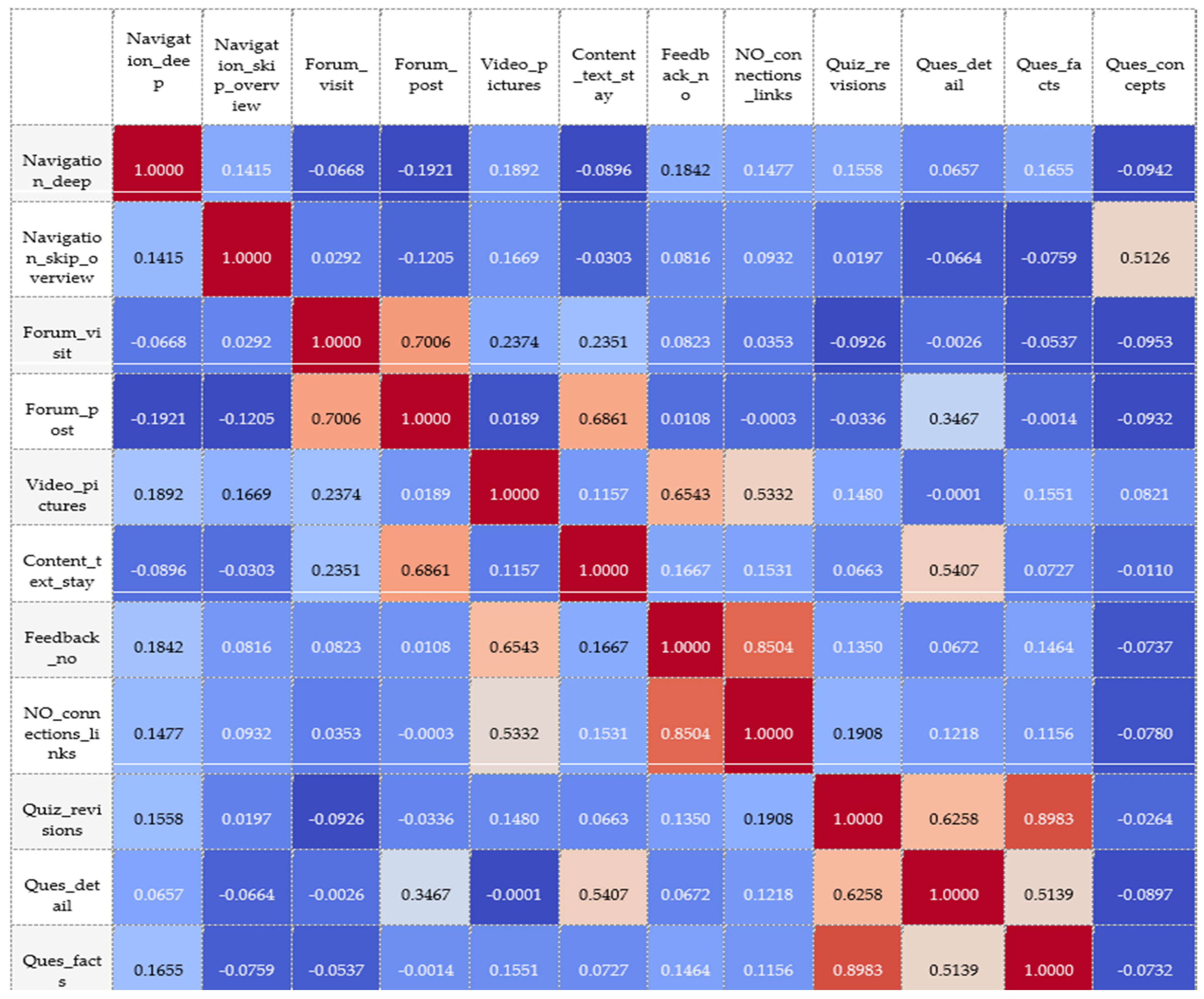
3.1. Exploratory Data Analysis and the Preprocessing of Input Features

For our experiments, we used an artificially generated data set: after generating the data set for a random multi-label classification problem, using the sklearn.datasets.make_multilabel_classification package, we adapted the data set to the students’ learning-style classification problem. This approach was applied due to the paucity of informative and representative data available in the actual Moodle environment. Samples were expertly labeled, manually, on the basis of the knowledge acquired in the course of our previous research, the results of which were published in [15]. In that research, we investigated the relationships between factors deduced from the students’ interactions with a virtual learning environment, by means of tracking each student’s behavior and learning style.
During the exploratory data analysis, the main statistical characteristics of the set of input features (activities of the student in the VLE) were identified—the results are presented in Table 1.
The mean (average) of a data set is found by adding all numbers in the data set and then dividing by the number of values in the set. The standard deviation (“std” in the Table 1.) is a statistic that measures the dispersion of a dataset relative to its mean and is calculated as the square root of the variance. The minimum (“min” in the Table 1) is the smallest value in the data set. Names of the input features are presented in the headings of the table—they are explained further in the Section 3.2.
The correlation matrix, once computed, shows 2 pairs of input features that tend to be strongly correlated (marked in dark red colour). The labels are not correlated (see Figure 1).
It is appropriate to note that, in general, depending on the data set available, it may be necessary to use input feature preprocessing techniques for cleaning up the data [38], feature scaling, imputing the missing values, for oversampling or under-sampling in the case of an imbalanced data set, encoding the categorical data, etc.

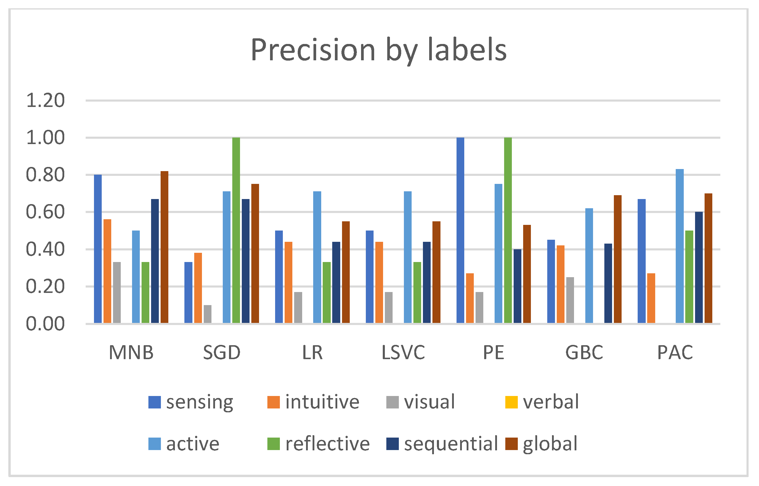
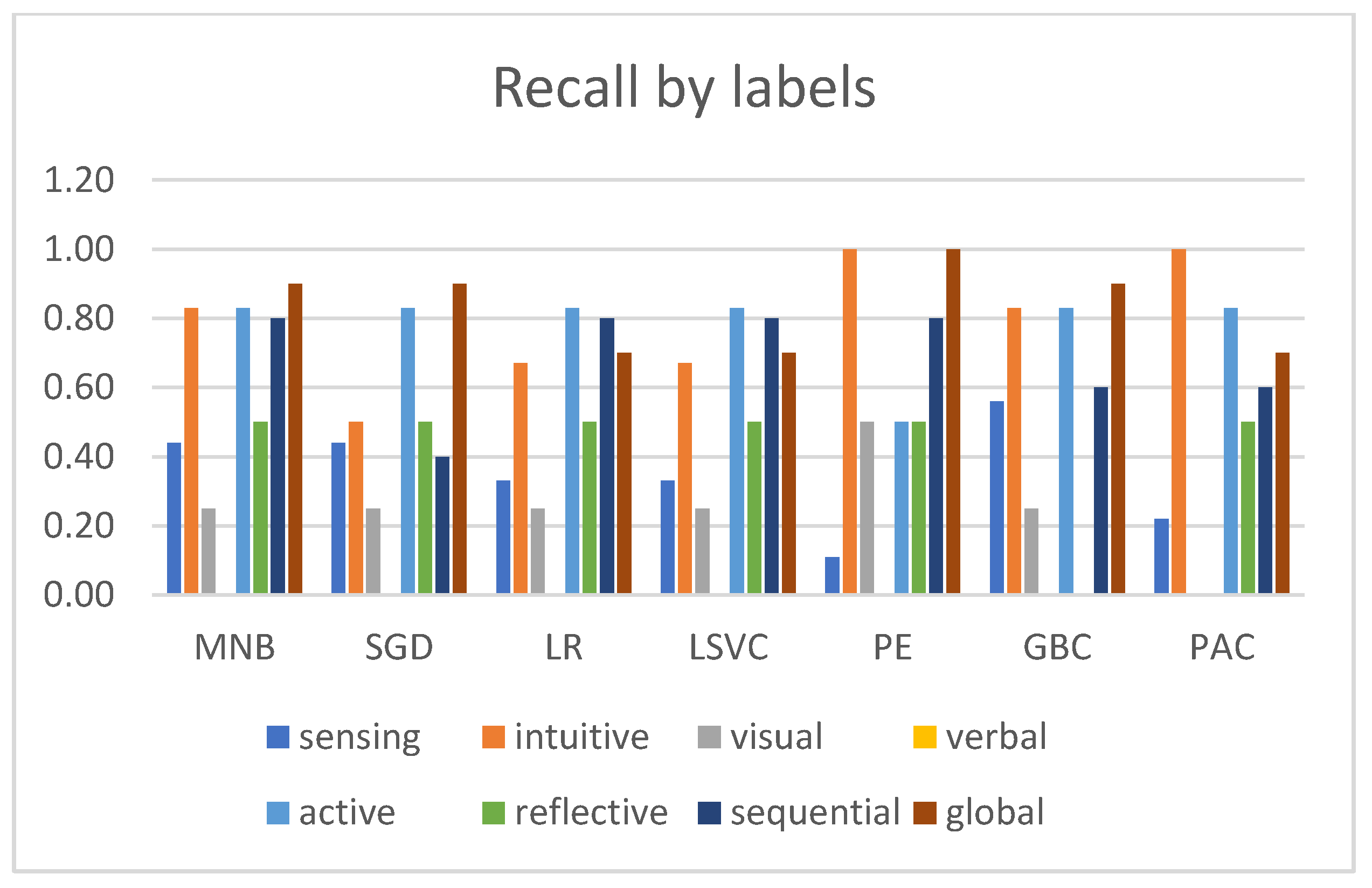
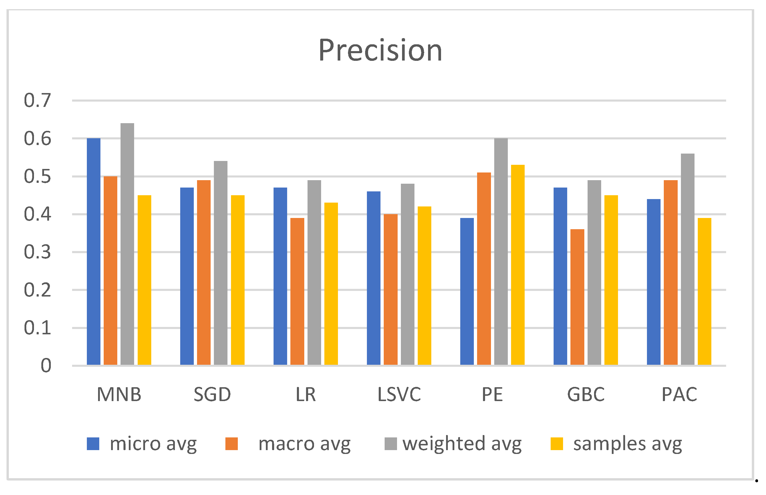
3.2. Experimental Evaluation and Comparative Analysis of Multi-Label Classifiers

In supervised machine learning, when choosing the best multi-label classification methods for student learning-style classification, it is necessary to consider problem transformation, algorithm adaptation, and ensemble methods. The computational complexity of the multi-label methods is presented in more detail in [16].
In order to evaluate and compare the capabilities of the various multi-label classifiers that use the problem transformation approach and the OneVsRest classification strategy, we trained the OneVsRest classifier using the following base estimators: Perceptron, MultinomialNB, SGDClassifier, LogisticRegression, LinearSVC, GradientBoostingClassifier, and PassiveAggressiveClassifier. The base estimators were fitted on random subsets of the dataset. During the experiment, the target variable was converted to a multi-label binarizer, then the OneVsRest classifiers were built on the above-mentioned estimators. Due to the fact that the data on students’ activities, stored in the real Moodle environment, are not informative enough and, because of that, the execution of the exploratory data analysis and data engineering tasks requires a substantial investment of time resources, we generated a synthetic data set and modified it to suit the classification of the students’ learning-style problem. Therefore, the experimental data were manually labeled, based on expert knowledge. The data set consists of 99 data samples with 12 features:
  • Navigation_deep—the depth of navigation (how much depth);
  • Navigation_skip_overview—the number of times that the student skips through the overview;
  • Forum_visit—the number of times that the student visited the forum;
  • Forum_post—the number of times that the student posted to the forum;
  • Video_pictures—the number of times that the student watched videos/pictures;
  • Content_text_stay—how long the student stayed on the content/topic;
  • Feedback_no—the number of times that the student submitted feedback;
  • NO_connections_links—the working time of the user with the weblinks tools—following a hyperlink to other learning material or web pages;
  • Quiz_revision—the number of times that the student visited quiz revision pages;
  • Ques_detail—the time spent on question details;
  • Ques_facts—the time spent on questions of the type, “facts”;
  • Ques_concepts—the time spent on questions of the type, “concepts”.
These features are informative and they characterize the corresponding learning styles. They are factors that influence the determination of a student’s learning style. The actual values of these factors may be deduced from the students’ interactions with the virtual learning environment, by means of tracking student behavior in the environment.
The combination of 8 class labels (sensing, intuitive, visual, verbal, active, reflective, sequential, and global) was expertly assigned for each sample. As a rough rule of thumb, the model should be trained on at least an order of magnitude (ten times) more examples than the trainable parameters. Simple models with large data sets may, generally, predict better than complex models using small data sets.
The measuring tools provided by sklearn [39] were used to measure the OneVsRestClassifier’s generalization ability:
  • Hamming loss—the fraction of labels that are incorrectly predicted, i.e., the fraction of the wrong labels compared to the total number of labels; this measures how well the classifier predicts each of the labels, averaged over samples, then over all labels;
  • Precision—this measures the fraction of relevant instances among the retrieved instances;
  • Recall—this measures the fraction of relevant instances that were retrieved;
  • The F1 score measures a weighted average of precision and recall, where both have the same impact on the score.
As the data set is small, each OneVsRestClassifier that uses another estimator as a parameter was evaluated using the hold-out method: the data set was split up into a “train” and “test” set. The training set is the data on which the model is trained, and the test set is used to see how well that model performs on unseen data. The evaluation results are presented in Figure 2, Figure 3, Figure 4, Figure 5, Figure 6, Figure 7 and Figure 8, below. According to the results, MultinomialNB and GradientBoostingClassifier should be preferred for the classification of learning styles as their F1 scores are the highest and their Hamming losses are the lowest. As we know from the theory, the Hamming loss is a better metric than accuracy for multi-label classification as, in the latter case, a misclassification is no longer a definite wrong or right answer [40,41]. Besides this, the Hamming loss is also used to measure the performance of imbalanced data set approaches [42].
Due to the large number of multi-label classification methods, for our algorithm adaptation methods, we relied on the evaluation results presented in [16]: RFPCT and BPNN are the best-performing methods. In order to experimentally test the application of neural networks for student learning-style detection, we constructed a fully connected neural network of 4 layers using a s i g m o i d activation function in the output layer and a r e l u activation function in the other layers. The s i g m o i d activation function was chosen because it most often showed a return value in the range of 0 to 1, and our task was to assign to each sample a set of probabilities for target labels corresponding to the student’s learning style (intuitive, sensing, verbal, active, global, sequential, reflective, or visual). The number of neurons in each layer was equal to the number of learning activities (this was 12). The batch size was 30. The He_uniform variance scaling initializer was used to set the initial random weights. The neural network was trained on the data of the same training data set that was used for applying the OneVsRest strategy. The data set has no missing values. The Binary_crossentropy loss function and adaptive moment estimation (Adam) learning method (optimizer = tf.keras.optimizers.Adam (lr = 0.0001)) was used, which computes adaptive learning rates for each parameter. With Adam, the learning rate may at first increase in the early layers; thus, helping to improve the efficiency of the deep neural network. The network converged after 30 epochs. In the NN, the correlation is taken into account since the hidden layers are summing all the input signals together via a fully connected layer. The neural network will learn about the co-occurrence of labels, finding some deterministic rules for generating the best output. The predictions of the model are presented in the form of “[0.991552591 0.599381804 0.772709548 0.0182502270 0.00593709946 0.112661839 0.981987536 0.987546802]” for every data sample, indicating the probability values for each learning-style class. The model was evaluated on the validation data set, using the repeated k-fold cross validator, which was repeated 5 times. The average model accuracy obtained was quite small—2.66. The reasons for that may be the small training data set, imperfect data labeling by the experts, insufficient feature engineering, and/or the imbalance of data. Besides, a change in the number of hidden layers or neurons, regularization, data normalization, and the application of principal component analysis could potentially improve the accuracy. The confusion matrix for the validation data set of the experimental NN is the following: [[68 0] [31 0]] [[57 0] [42 0]] [[9 89] [0 1]] [[0 69] [0 30]] [[81 0] [18 0]] [[91 0] [8 0]] [[0 76] [0 23]] [[0 68] [0 31]]. Other multi-labeled classification metrics were calculated for the model as well—the classification summary is presented in Table 2.
The Hamming loss, i.e., the fraction of labels that are incorrectly predicted, is 0.5.
Considering the ensemble methods [28], it is worth mentioning the classifier chains and other methods that are applicable for cases when the labels are correlated [43,44]. Classifier chains combine a number of binary classifiers into a single multi-label model that is capable of exploiting the correlations among targets. The predictions of each model are passed on to the subsequent models in the chain, to be used as features [18].
It is relevant for the teacher who prepares the learning objects and learning paths, using the predictions of the multi-label classification model to know how each feature affects the prediction of a data point. The method most suitable for this purpose in the case when students’ activities (input features) are weakly correlated is SHAP. The goal of SHAP is to explain the prediction of an instance by computing the contribution of each feature to the prediction. The Shapley value of a feature value is its contribution to the payout, weighted and summed over all possible feature value combinations. SHAP values interpret the impact of having a certain value assigned to a given feature, in comparison to the prediction we would make if that feature had some baseline value. In other words, SHAP values show how much a given feature has changed our prediction (compared to if we had made that prediction at some baseline value of that feature).
We applied the generic shap.KernelExplainer to explain the predicted results of the NN model that was trained and used in the experiment. According to the SHAP documentation, kernel SHAP is a method that uses a special weighted local linear regression to compute the importance of each feature. The Deep Explainer may also be the best option for the NN. We achieved a ( n _ s a m p l e s , n _ f e a t u r e s ) NumPy array, each element of which is the Shapley value of that feature of the corresponding record (sample). The summary plot of Shapley values is presented in Figure 9. Features with large, absolute Shapley values are important. If we want to establish global importance, we average the absolute Shapley values per feature across the data.
The SHAP summary plot combines feature importance with feature effects: each point on the summary plot is a Shapley value for a feature and an instance. The color represents the value of the feature, from low to high. SHAP also presents the possibility of visualizing the feature’s importance for each target label. We drew summary plots for intuitive, sensing, verbal, active, global, sequential, reflective, and visual learning styles. The example for “sensing” the target is presented in Figure 10.
In the plot for this particular target label, the high values of the feature (indicated by the rose/purple combination) led us to prediction 1: low values of the feature (indicated by blue) leads to the prediction, 0. Such a visualization would help teachers to quickly perform the SHAP analysis and detect which features were most important, i.e., which contributed the most to the prediction of the probability value of the corresponding learning style.
It must be stressed that, as when citing [45], “SHAP only tells you what the model is doing within the context of the data on which it has been trained: it doesn’t necessarily reveal the true relationship between variables and outcomes in the real world”. Therefore, SHAP is not the best choice when wishing to engineer specific outcomes by manipulating features (unless the experiment is being conducted within the causal framework), but it may be useful for making a machine learning model more explainable by visualizing its output. Explanations presenting the contribution of each activity in the VLE to the prediction of the learning style of the student may enable teachers and other users to better understand what led to the corresponding learning style of the learner and to adjust their activities accordingly, in order to adapt the virtual learning environment to the student’s learning style.
The procedures, methods, and tools described in the paper should provide guidance for teachers and other users in practically personalizing the virtual learning environment, and attention must be drawn to that in practice; learning material is usually created for a particular group of learners. We can use the stacked SHAP explanations and cluster data, with the help of Shapley values, for that purpose (Figure 11). The goal of clustering is to find groups of similar instances. Normally, clustering is based on features. SHAP clustering works by clustering the Shapley values of each instance. This means that we cluster instances according to explanation similarity. Such a force plot shows how features explain the model output for multiple observations at the same time. The red SHAP values in the plot increase the prediction, while the blue values decrease it.
Force plots showing the contribution of each feature to the prediction of the corresponding label (Figure 12) are also informative; therefore, they are applicable for practical use by teachers.

4. Discussion and the Methodology Proposed

4.1. Mechanisms to Select the Appropriate Machine Learning Methods for Student Learning-Style Prediction and Interpretation

Based on the findings from our literature-based research, and using the results of our experiments, we see that the different preprocessing, classification, or clustering and interpretation methods have to be applied depending on the peculiarities of the data set (imbalanced or not, sparse or not, having missing values or not, having correlated features or not, having correlated labels or not, etc.) and the specifics of the multi-label classification and model interpretation tasks that need to be performed. We identified from our experiments that the MultinomialNB and GradientBoostingClassifier performed best when applying the One-vs-all strategy. The authors of [46] state that “the binary relevance method, specifically One-vs-all, yields the best result in the real data analysis, but has the drawback of neglecting correlation among labels. The label powerset considers correlations between labels indirectly but has the drawback of not including all possible label combinations in the model-fitting process, which leads to overfitting of the training set”. Based on the literature review, we know that the ensemble of classifier chains (ECC) algorithm is very effective for multi-labeled learning objects; therefore, it is proposed as the best classification algorithm for data sets with correlated labels, followed by RAKEL, ML-kNN, and finally, EPS [47]. ML-kNN performs the worst, but it has the advantage of producing a ranking of the labels. Based on the work in [48], “the ECC has the best performance in all measures, followed by EPS and RAKEL. However, with respect to the Hamming loss, the RAKEL and ML-KNN are the best-performing methods, followed by ECC. As for the label-based evaluation measures, the best-performing methods are ECC and BR”. Empirical evidence published by [49] shows that ML-kNN performs the best, followed by RAKEL, then followed by the classifier chain and binary relevance. The authors of [50] emphasize that BR methods are quite appropriate for a not very large number of labels and that they have strong limitations regarding the use of label relationship information. They propose the BR+ approach, to improve the multi-label classification performance in datasets that do not have a very high label space dimensionality, trying to discover label dependency. The authors of [51] experimentally prove that, for data sets with correlated labels, the LC and PS methods give better prediction results than the BR method as the LC and PS consider label correlation during the transformation from a multi-label to a single-label dataset. A comprehensive comparison between various problem transformation methods is presented in [52]. It states the merits and/or disadvantages of the classification methods as the ability to utilize the available unlabeled data for classification, the ability to take label correlations into account, and the speed and computational complexity of each problem transformation method. Complexity comments on the multi-label classification algorithms are also presented by the authors of [24].
Various model interpretation approaches may be chosen for explaining the predicted students’ learning styles as well. Except for those cases when we have inherently interpretable models (such as BCM) with imposed interpretability constraints, model-agnostic explanation methods may be used for interpreting the model. These methods are considered post hoc since they are decoupled from the black box [35].
Systematizing the research results, we present the procedure that might be followed for the selection of methods for multi-label students’ learning-style detection and interpretation (Figure 13).

4.2. Threats to Validity

It is stated by Maheswari in [53] that the size of the data set may manifest issues relating to generalization, data imbalance, and difficulty in reaching the global optimum. A large dataset helps to avoid overfitting and generalizes better as it captures the inherent data distribution more effectively [53]. The authors of this paper are aware of that issue and know that this also applies to the experiments described in this article. In our opinion, the small size of the data set is one of the reasons why the NN prediction accuracy obtained is not high. In summary, larger data sets may influence the pattern learned; however, this does not fundamentally change the applicability of the particular approaches and/or methods for the learner’s learning-style prediction. As has already been stated in this paper, tuning the hyper-parameters of the model (for a NN, the change in the number of hidden layers or neurons), regularization, data normalization, and the application of principal component analysis could also potentially improve the prediction accuracy.

5. Conclusions

Multi-label classification methods may be applied for student learning-style prediction. In cases where the data set is balanced and the labels are independent, one of the most popular of the problem transformation strategies—the OneVsRest strategy—is appropriate for the classification of students’ learning activities and student learning-style identification. The problem transformation approach is also suggested in cases when there is a relatively small number of learning-style classes (OneVsRest learns n binary classifiers ( n is the number of classes in a dataset), one for each label from all instances of the original dataset). Empirical research shows that the MultinomialNB or GradientBoostingClassifier should be preferred as a base estimator as the fraction of labels that were incorrectly predicted by the OneVsRestClassifier, which uses the MultinomialNB or GradientBoostingClassifier, is the lowest, while the harmonic mean of precision and recall is the highest. One more advantage of the OneVsRest approach is its interpretability: since each class is represented by one and only one classifier, it is possible to gain knowledge about the class by inspecting its corresponding classifier. When the labels are correlated [54], a chain of binary classifiers should be constructed, wherein a classifier C i uses the predictions of all the classifiers, C j , where j < i , or the label-powerset method is chosen. It must be noted that the chain of binary classifiers does not utilize unlabeled data.
In order to avoid high resource consumption when applying the OneVsRest strategy, problem adaptation methods may be used instead of problem transformation methods. By experimenting with a neural network, we showed that the use of a series of NN algorithms to recognize the underlying relationships in a set of labeled students’ learning activity data and to predict the probabilities of student learning-style dimensions is appropriate and applicable. The low performance accuracy of the constructed NN forces us to conclude that the size of the data set may manifest issues relating to generalization.
When the student’s activities (the input features) are not strongly correlated, the SHAP method is the best option in order to provide teachers with a better understanding of what historical activities in the virtual learning environment were most favored by the student. In the case of a strong correlation, other interpretation methods must be chosen.
We plan to experiment with interpretation methods that address the problem of strongly correlated data features in the future. After that, we are going to explore the application of ensemble methods using the two approaches: the averaging approach and the combination of several weaker models to produce a powerful ensemble.

Author Contributions

Conceptualization, D.G.; methodology, D.G.; validation, D.G. and L.S.; formal analysis, D.G.; investigation, D.G.; resources, D.G. and L.S.; writing—original draft preparation, D.G.; writing—review and editing, D.G.; visualization, D.G.; All authors have read and agreed to the published version of the manuscript.

Funding

This research received no external funding.

Institutional Review Board Statement

Not applicable.

Informed Consent Statement

Not applicable.

Data Availability Statement

Data available on request.

Conflicts of Interest

The authors declare no conflict of interest.

Abbreviations

NNNeural network
BCMBayesian case model
BPNNBackpropagation neural network
SHAPShapley additive explanations
MLCMulti-label classification
SVMSupport vector machines
ML-kNNMulti-label k-nearest neighbor
PSPruned sets
EPSEnsembles of pruned sets
BRBinary relevance
RAKELRandom k-label sets
LP (LC)Label powerset (label combination)
NBNaïve Bayes

References

  1. Gambo, Y.; Shakir, M.Z. An Artificial Neural Network (ANN)-Based Learning Agent for Classifying Learning Styles in Self-Regulated Smart Learning Environment. Int. J. Emerg. Technol. Learn. (IJET) 2021, 16, 185–199. [Google Scholar] [CrossRef]
  2. Gomede, E.; Miranda de Barros, R.; de Souza Mendes, L. Use of Deep Multi-Target Prediction to Identify Learning Styles. Appl. Sci. 2020, 10, 1756. [Google Scholar] [CrossRef] [Green Version]
  3. Nasiri, J.; Mir, A.M.; Fatahi, S. Classification of learning styles using behavioral features and twin support vector machine. Technol. Educ. J. (TEJ) 2008, 13, 316–326. [Google Scholar] [CrossRef]
  4. Sasidhar, R.C.; Arunachalam, A. Personalization of Learning Management System using VARK. Turk. J. Comput. Math. Educ. 2021, 12. [Google Scholar] [CrossRef]
  5. Zhang, Y.; Dai, H.; Yun, Y.; Liu, S.; Lan, A.; Shang, X. Meta-knowledge dictionary learning on 1-bit response data for student knowledge diagnosis. Knowl. Based Syst. 2020, 205, 106290. [Google Scholar] [CrossRef]
  6. Zhang, Y.; An, R.; Liu, S.; Cui, J.; Shang, X. Predicting and Understanding Student Learning Performance Using Multi-sourse Sparse Attention Convolutional Neural Networks. IEEE Trans. Big Data 2021, 1. [Google Scholar] [CrossRef]
  7. Lwande, C.; Muchemi, L.; Oboko, R. Identifying learning styles and cognitive traits in a learning management system. Heliyon 2021, 7, e07701. [Google Scholar] [CrossRef]
  8. Dung, P.Q.; Florea, A.M. An approach for detecting learning styles in learning management systems based on learners’ behaviours. Int. Conf. Educ. Manag. Innov. 2012, 30, 171–177. [Google Scholar]
  9. Preidys, S.; Sakalauskas, L. Possibilities of integrating of smart modules into VMA Moodle: From theory to practice [Capabilities for Intelligent Modules Integration into the Moodle VLE: From Theory to Practice]. Mokslo taikomųjų tyrimų įtaka šiuolaikiniųn studijų kokybei 2012, 1, 77–82. [Google Scholar]
  10. Wang, J.; Mendori, T. The reliability and validity of Felder-Silverman Index of learning styles in Mandarin version. Int. J. Inf. Eng. Express 2015, 1, 1–8. [Google Scholar] [CrossRef]
  11. Brownlee, J. Tour of Evaluation Metrics for Imbalanced Classification. Machine Learning Mastery. Imbalanced Classification. 2020. Available online: https://machinelearningmastery.com/tour-of-evaluation-metrics-for-imbalanced-classification/ (accessed on 23 May 2022).
  12. Preidys, S.; Sakalauskas, L. Analysis of students’ study activities in virtual learning environments using data mining methods. Technol. Econ. Dev. 2010, 16, 94–108. [Google Scholar] [CrossRef]
  13. Ghamrawi, N.; McCallum, A. Collective multi-label classification. In Proceedings of the 14th ACM International Conference on Information and Knowledge Management, ACM, Atlanta, GA, USA, 17–22 October 2005. [Google Scholar]
  14. Godbole, S.; Sunita, S. Discriminative methods for multi-labeled classification. In Advances in Knowledge Discovery and Data Mining; Springer: Berlin/Heidelberg, Germany, 2004. [Google Scholar]
  15. Goštautaitė, D. Dynamic learning style modelling using probabilistic Bayesian network. Edulearn 2019, 2921–2932. [Google Scholar] [CrossRef]
  16. Bogatinovski, J.; Todorovski, L.; Džeroski, S.; Kocev, D. Comprehensive Comparative Study of Multi-Label Classification Methods. Comput. Sci. 2021, 203. [Google Scholar] [CrossRef]
  17. Kravcik, M.; Angelova, G.; Ceri, S.; Cristea, A.; Damjanović, V.; Devedžić, V.; Dimitrova, V.; Dolog, P.; Đurić, D.; Ga Ević, D.; et al. Requirements and Solutions for Personalized Adaptive Learning. 2005. Available online: https://hal.archives-ouvertes.fr/hal-00590961/ (accessed on 23 May 2022).
  18. Scikit-Learn. Multiclass and Multioutput Algorithms. Available online: https://scikit-learn.org/stable/modules/multiclass.html (accessed on 23 May 2022).
  19. Read, J.; Pfahringer, B.; Holmes, G.; Frank, E. Classifier chains for multi-label classification. Mach. Learn. 2011, 85, 333–359. [Google Scholar] [CrossRef] [Green Version]
  20. Bernard, J.; Chang, T.; Popescu, E.; Graf, S. Learning style Identifier: Improving the precision of learning style identification through computational intelligence algorithms. Expert Syst. Aapli. 2017, 75, 94–108. [Google Scholar] [CrossRef]
  21. Wikipedia: Earning Styles. 2022. Available online: https://en.wikipedia.org/wiki/Learning_styles (accessed on 23 May 2022).
  22. Pushpa, M.; Karpagavalli, S. Multi-label Classification: Problem Transformation methods in Tamil Phoneme classification. Procedia Comput. Sci. 2017, 115, 572–579. [Google Scholar] [CrossRef]
  23. Sawsan, K. Learning methods for multi-label classification. In Machine Learning [stat.ML]; Université de technologie de Compiègne: Compiègne, France; Université Libanaise: Beirut, Liban, 2013. [Google Scholar]
  24. Mohammad, S. A literature survey on algorithms for multi-label learning. Comput. Sci. 2021, 18, 1–25. [Google Scholar]
  25. Al-Otaibi, R.; Flach, P.; Kull, M. Multi-label Classification: A Comparative Study on Threshold Selection Methods. In Proceedings of the First International Workshop on Learning over Multiple Contexts (LMCE) at ECML-PKDD as Part of the 7th European Machine Learning and Data Mining Conference (ECML-PKDD 2014), Nancy, France, 14–18 September 2014. [Google Scholar]
  26. Rasheed, F.; Wahid, A. Learning style detection in E-learning systems using machine learning techniques. Expert Syst. Appl. 2021, 74, 114774. [Google Scholar] [CrossRef]
  27. Zhang, M.; Zhou, Z. A Review on Multi-Label Learning Algorithms. IEEE Trans. Knowl. Data Eng. 2014, 26, 1819–1837. [Google Scholar] [CrossRef]
  28. Madjarov, G.; Kocev, D.; Gjorgjevikj, D.; Džeroski, S. An extensive experimental comparison of methods for multi-label learning. Pattern Recognit. 2012, 45, 3084–3104. [Google Scholar] [CrossRef]
  29. Nooney, K. Deep dive into multi-label classification..! (With detailed Case Study). Available online: https://towardsdatasciencecom/journey-to-the-center-of-multi-label-classification-384c40229bff (accessed on 23 May 2022).
  30. Prathibhamol, C.P.; Jyothy, K.V.; Noora, B. Multi label classification based on logistic regression (MLC-LR). In Proceedings of the International Conference on Advances in Computing, Communications and Informatics (ICACCI), Jaipur, India, 21–24 September 2016. [Google Scholar]
  31. Goštautaitė, D.; Kurilov, J. Comparative Analysis of Exemplar-Based Approaches for Students’ Learning Style Diagnosis Purposes. Appl. Sci. 2021, 11, 7083. [Google Scholar] [CrossRef]
  32. Tsoumakas, G.; Ioannis, K. Multi-label classification: An overview. Comput. Sci. 2006. [Google Scholar] [CrossRef] [Green Version]
  33. Aas, K.; Jullum, M.; Løland, A. Explaining individual predictions when features are dependent: More accurate approximations to Shapley values. Artif. Intell. 2021, 298, 103502. [Google Scholar] [CrossRef]
  34. Molnar, C. A Guide for Making Black Box Models Explainable. Available online: https://christophm.github.io/interpretable-ml-book/index.html#summary (accessed on 23 May 2022).
  35. Carvalho, V.; Pereira, M.; Cardoso, S. Machine Learning Interpretability. A Survey onMethods and Metrics. Electronics 2019, 8, 832. [Google Scholar] [CrossRef] [Green Version]
  36. Mase, M.; Owen, A.; Seiler, B. Explaining Black Box Decisions by Shapley Cohort Refinement. 2019. Available online: https://arxiv.org/abs/1911.00467 (accessed on 23 May 2022).
  37. Basu, I.; Maji, S. Multicollinearity Correction and Combined Feature Effect in Shapley Values. arXiv 2020, arXiv:2011.01661. [Google Scholar]
  38. Maaliw, I.; Renato, R.; Ballera, M.; Ambat, S.; Dumlao, M. Comparative Analysis of Data Mining Techniques for Classification of Student’s Learning Styles. In Proceedings of the 5th International Conference on Advances in Science, Engineering and Technology (ICASET-17), Manila, Philippines, 18–19 September 2017. [Google Scholar]
  39. Bogatinovski, J.; Todorovski, L.; Džeroski, S.; Kocev, D. Explaining the Performance of Multi-label Classification Methods with Data Set Properties. Int. J. Intell. Sytems 2021. [Google Scholar] [CrossRef]
  40. Sharat, C. Hamming Score for Multi-Label Classification. 2021. Available online: https://www.linkedin.com/pulse/hamming-score-multi-label-classification-chandra-sharat (accessed on 23 May 2022).
  41. Wu, G.; Zhu, J. Multi-label classification: Do Hamming loss and subset accuracy really conflict with each other? In Proceedings of the Advances in Neural Information Processing Systems 33 (NeurIPS 2020), Virtual, 6–12 December 2020. [Google Scholar]
  42. Winata, G.I.; Khodra, M.L. Handling Imbalanced Dataset in Multi-label Text Categorization using Bagging and Adaptive Boosting. Int. Conf. Electr. Eng. Inform. 2015, 500–505. [Google Scholar] [CrossRef] [Green Version]
  43. Dembczyński, K.; Waegeman, W.; Cheng, W.; Hüllermeier, E. On label dependence and loss minimization in multi-label classification. Mach. Learn. 2012, 88, 5–45. [Google Scholar] [CrossRef] [Green Version]
  44. Wang, S.; Wang j Wang, Z.; Ji, Q. Enhancing multi-label classification by modeling dependencies among labels. Comput. Sci. Pattern Recognit 2014, 47, 3405–3413. [Google Scholar] [CrossRef]
  45. Cooper, A. Ideas, Explorations and Musings on Data. 2021. Available online: https://www.aidancooper.co.uk/a-non-technical-guide-to-interpreting-shap-analyses/ (accessed on 23 May 2022).
  46. Comparision of Four Multilabel-Classification Methods. 2019. Available online: https://www.causeweb.org/usproc/sites/default/files/usclap/2019-1/Comparison%20of%20Four%20Multi-Label%20Classification%20Methods.pdf (accessed on 23 May 2022).
  47. Aldrees, A.; Chikh, A.; Berri, J. Comparative evaluation of four multilabel classification algorithms in classifying learning objects. Comput. Sci. Inf. Technol. (CS IT) 2016, 24, 651–660. [Google Scholar]
  48. Elkafrawy, P.; Mousad, A. Experimental comparision of methods for multi-label classification in different application domains. Int. J. Comput. Appl. 2015, 114, 1–9. [Google Scholar]
  49. Tawiah, C.A.; Sheng, V.S. Empirical comparision of multilabel-classification algorythms. In Proceedings of the Association for the Advancement of Artificial Intelligence Conference on Artificial Intelligence, Bellevue, WA, USA, 14–18 July 2013. [Google Scholar]
  50. Cherman, E.A.; Monard, M.C.; Metz, J. Multi-label Problem Transformation Methods: A Case Study. CLEI Electron. J. 2011, 14, 4. [Google Scholar] [CrossRef] [Green Version]
  51. Modi, H.; Panchal, M. Experimental Comparison of Different Problem Transformation Methods for Multi-Label Classification using MEKA. Int. J. Comput. Appl. 2012, 59, 10–15. [Google Scholar] [CrossRef]
  52. Nareshpalsingh, J.; Modi, H. Multi-label classification methods: A comparative study. Int. Res. J. Eng. Technol. 2017, 4, 263–270. [Google Scholar]
  53. Maheswari, J.P. Breaking the Curse Of Small Data Sets In Machine Learning. Why the Size of Data Matters and How to Work with Smalll Data. 2018. Available online: https://towardsdatascience.com/breaking-the-curse-of-small-datasets-in-machine-learning-part-1-36f28b0c044d (accessed on 23 May 2022).
  54. Cherman, E.; Metz, J.; Monard, M. A Simple Approach to Incorporate Label Dependency in Multi-label Classification. In Proceedings of the 9th Mexican International Conference on Artificial Intelligence Conference on Advances in Soft Computing: Part II, Pachuca, Mexico, 8 November 2010. [Google Scholar]
Figure 1. Correlation matrix.
Applsci 12 05396 g001
Figure 2. Hamming losses and Hamming scores of the OneVsRestClassifier, which uses another estimator as a parameter.
Applsci 12 05396 g002
Figure 3. Precision values according to the labels of the OneVsRestClassifier, which uses another estimator as a parameter.
Applsci 12 05396 g003
Figure 4. Recall values according to the labels of the OneVsRestClassifier, which uses another estimator as a parameter.
Applsci 12 05396 g004
Figure 5. F1 score values according to the labels of the OneVsRestClassifier, which uses another estimator as a parameter.
Applsci 12 05396 g005
Figure 6. Precision averages of the OneVsRestClassifier, which uses another estimator as a parameter.
Applsci 12 05396 g006
Figure 7. Recall averages of the OneVsRestClassifier, which uses another estimator as a parameter.
Applsci 12 05396 g007
Figure 8. F1 score averages of the OneVsRestClassifier, which uses another estimator as a parameter.
Applsci 12 05396 g008
Figure 9. Global SHAP summary plot.
Applsci 12 05396 g009
Figure 10. SHAP summary plot for the “sensing” learning style.
Applsci 12 05396 g010
Figure 11. Stacked SHAP values and cluster data.
Applsci 12 05396 g011
Figure 12. The SHAP force plot for the “sensing” learning style.
Applsci 12 05396 g012
Figure 13. Procedure for selection of methods for multi-label students’ learning style detection [1,36].
Applsci 12 05396 g013
Table 1. Statistical characteristics of the sets of input features.
Navigation DeepNavigation Skip OverviewForum VisitForum PostVideo, PicturesContent Text StayFeedback No.No. of _Connections or LinksQuiz RevisionQuestion Details
mean7.37378.58588.272710.72724.68688.85855.37375.33338.080810.7373
std5.77926.01706.11257.02303.72977.10704.60164.77875.70116.3576
min1.00001.00001.00001.00001.00001.00001.00001.00001.00001.0000
25%2.00003.00003.00004.00002.00002.00002.00002.00003.00004.0000
50%6.00008. 00007.00009.00004.000070.0004.00004.00006.000011.0000
75%11.500014.500012.500018.00007.500017.00008.00007.500014.000016.0000
max20.000020.000020.000020.000020.000020.000020.000020.000020.000020.0000
Table 2. NN model classification report.
Learning StylePrecisionRecallF1 ScoreSupport
sensing0.860.810.8331
intuitive0.840.880.8642
visual0.000.000.001
verbal0.970.930.9530
active0.930.720.8118
reflective0.000.000.008
sequential0.730.350.4723
global0.850.710.7731
Micro avg.0.860.720.79184
Macro avg.0.650.550.59184
Weighted avg.0.820.720.76184
Samples avg.0.710.640.66184
Publisher’s Note: MDPI stays neutral with regard to jurisdictional claims in published maps and institutional affiliations.

