Optimization Workflows for Linking Model-Based Systems Engineering (MBSE) and Multidisciplinary Analysis and Optimization (MDAO)

Abstract

Developing modern products involves numerous domains (controlling, production, engineering, etc.) and disciplines (mechanics, electronics, software, etc.). The products have become increasingly complex while their time to market has decreased. These challenges can be overcome by Model-Based Systems Engineering (MBSE), where all development data (requirements, architecture, etc.) is stored and linked in a system model. In an MBSE system model, product requirements at the system level can lead to numerous technical variants with conflicting objectives at the parameter level. To determine the best technical variants or tradeoffs, Multidisciplinary Analysis and Optimization (MDAO) is already being used today. Linking MBSE and MDAO allows for mutually beneficial synergies to be expected that have not yet been fully exploited. In this paper, a new approach to link MBSE and MDAO is proposed. The novelty compared to existing approaches is the reuse of existing MBSE system model data. Models developed during upstream design and test activities already linked to the MBSE system model were integrated into an MDAO problem. Benefits are reduced initial and reconfiguration efforts and the resolution of the MDAO black-box behavior. For the first time, the MDAO problem was modeled as a workflow using activity diagrams in the MBSE system model. For a given system architecture, this workflow finds the design variable values that allow for the best tradeoff of objectives. The structure and behavior of the workflow were formally described in the MBSE system model with SysML. The presented approach for linking MBSE and MDAO is demonstrated using an example of an electric coolant pump.

1. Introduction

1.1. Motivation

Boundary conditions such as increasingly stringent emissions legislation and advancing urbanization pose technological challenges for the automotive industry. In addition, stakeholder requirements regarding functionality, quality, and cost-efficiency are increasing [1]. These challenges are increasingly being met by four key trends [2]: electrification, autonomous driving, connected vehicles, and shared mobility. All these trends require the use of mechanical, electronic, and software systems onboard the automobile. Because of the progressive integration of these systems, modern vehicles can be understood as cyber-physical systems (CPS) [3]. A key characteristic of CPS is their complexity [4,5]. The increasing implementation of the aforementioned trends leads to an increasing system complexity of vehicles and their systems, which must be managed in development [6]. Furthermore, the rapid development and innovation of technologies lead to ever-increasing technological change [7]. To remain competitive in the market, automotive original equipment manufacturers (OEMs) and suppliers must not only continuously innovate but also keep the time to market short despite increasing complexity [8]. Cost, schedule, and scope overruns of projects are often attributed to unmanaged complexity [9]. Overall, companies are under pressure to develop innovative, complex products in ever shorter timeframes. The well-known development approach of Model-Based Systems Engineering (MBSE) offers the potential to make complexity manageable during the development of automotive products [10]. In MBSE, development data is continuously linked in a central MBSE system model compared to document-based, classical development approaches. In this case, “a system model is a representation of the target system or one or more of its subsystems” [11]. It combines domain-specific and domain-independent parts (simulation models), structures (architectures), and artifacts [11]. Development projects using MBSE are characterized, among other things, by improved traceability and consistency in a rigorous MBSE system model and the reuse of development data and models [12]. As a result, MBSE can help to reduce development time and cost [13,14,15]. System modeling with MBSE is mostly realized in the universal, graphical modeling language SysML. SysML thereby emphasizes aspects of system architecting [16] but lacks in providing analytical and numerical methods. Such methods are provided by using additional tools and toolchains [17]. These methods include sensitivity analyses, searching design spaces for optimal solutions, and trade studies [18], among others [19]. This lack of integration leads to a gap between system architecting and system analysis [16]. A similar gap persists between system architecting in MBSE and system analysis using domain-specific simulation models [20].

If requirements are formulated at the system level, with system design it is possible to identify numerous technical variants that differ in their design variables. Fulfilling the requirements of these technical variants can be conflicting, and a conflict of objectives can arise that must be resolved appropriately. Since MBSE methods are usually employed to design a small number of variants, only a few variants may be found that meet the requirements. Accordingly, the best possible objective values are unknown, and the conflict of objectives cannot be resolved in the best possible way. To identify technical variants with the best possible objective values, Multidisciplinary Analysis and Optimization (MDAO) methods are already being used today [21]. MDAO is an engineering discipline that uses numerical optimization to design multidisciplinary systems [22]. It can examine large areas of the design variable space. With MDAO, technical variants with optimal objective values can be found, and the conflict of objectives can be resolved with a suitable tradeoff. MDAO is considered in the literature to be both a method [23] and a tool [24] in developing complex products. MDAO requires a high initial effort, which for example, in aviation, can take 60–80% of the project time [25]. When MDAO is used in the development process, the implementation [22] and the principles considered are often only partially formalized [25]. MDAO is then a black box on which changes such as extensions, detailing, and maintenance are time-consuming to implement.

To solve this problem, MBSE can be used in conjunction with MDAO, and this linking has many advantages. By formalizing an MDAO problem in the MBSE system model, its black box behavior can be resolved. The formalization simplifies changes to the MDAO problem, such as extensions, detailing, and maintenance, thus reducing the reconfiguration effort. The initial effort of implementing an MDAO problem can also be reduced as development data and models already available in the MBSE system model can be reused.

1.2. Problem Statement

Deploying MDAO in system development allows to explore large parts of the design space, identify technical variants with the best objective values and resolve conflicting objectives appropriately. However, several challenges arise in classical document-centered system development approaches (Figure 1, left). These include for MDAO:

• high initial efforts due to distributed data
• high reconfiguration efforts
• black box behavior due to lack of formalization

Figure 1. (Left): MDAO in document-centered development. Scattered data and black box behavior. (Right): MDAO in model-based development. Single source of data and resolved black box behavior.

Figure 1. (Left): MDAO in document-centered development. Scattered data and black box behavior. (Right): MDAO in model-based development. Single source of data and resolved black box behavior.

The high initial effort arises in the setup of MDAO. Various development data of the system are required for MDAO. This includes, among others, requirements, models and parameter sets. This development data is usually distributed among different sources and participants in the project and must be gathered costly. Once executed, the results of MDAO must be distributed accordingly to each development data source with corresponding effort. Which development data and system aspects are ultimately included in MDAO and how they are linked is often not formalized, so MDAO exhibits black box behavior. The high reconfiguration effort arises because changes to development data are communicated via several different paths. The lack of formalization makes it difficult to implement changes.

The linking of MDAO and MBSE is shown in Figure 1, right. In this case, the MBSE system model acts as a single source of truth (SSO) for MDAO, as all data (requirements, models, …) related to the developed product are centrally stored. The initial effort for MDAO is reduced because the required development data exists in the MBSE system model in parts or completely [26]. Results of MDAO are systematically transferred to the linked model elements of the system architecture. The formalization of MDAO in the MBSE system model resolves its black box behavior. Therefore, which and how development data are considered in MDAO is always traceable. Changes to the development data have an immediate effect on MDAO, so that the reconfiguration effort of the MDAO problem is reduced. Due to these benefits, numerous research engages with methods for linking MBSE and MDAO.

1.3. Contribution

Section 5 provides a review of previous research linking MBSE and MDAO. However, existing approaches insufficiently address development data (e.g., models) reused from system development activities. As a result, existing potentials to reduce the initial implementation effort of MDAO remain untapped. Therefore, the following research question shall be answered in this paper:

How to link MDAO to MBSE system models taking advantage of existing models?

The following main contributions are made to answer the research question:

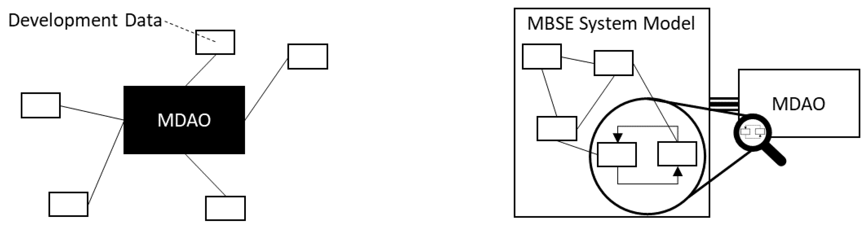
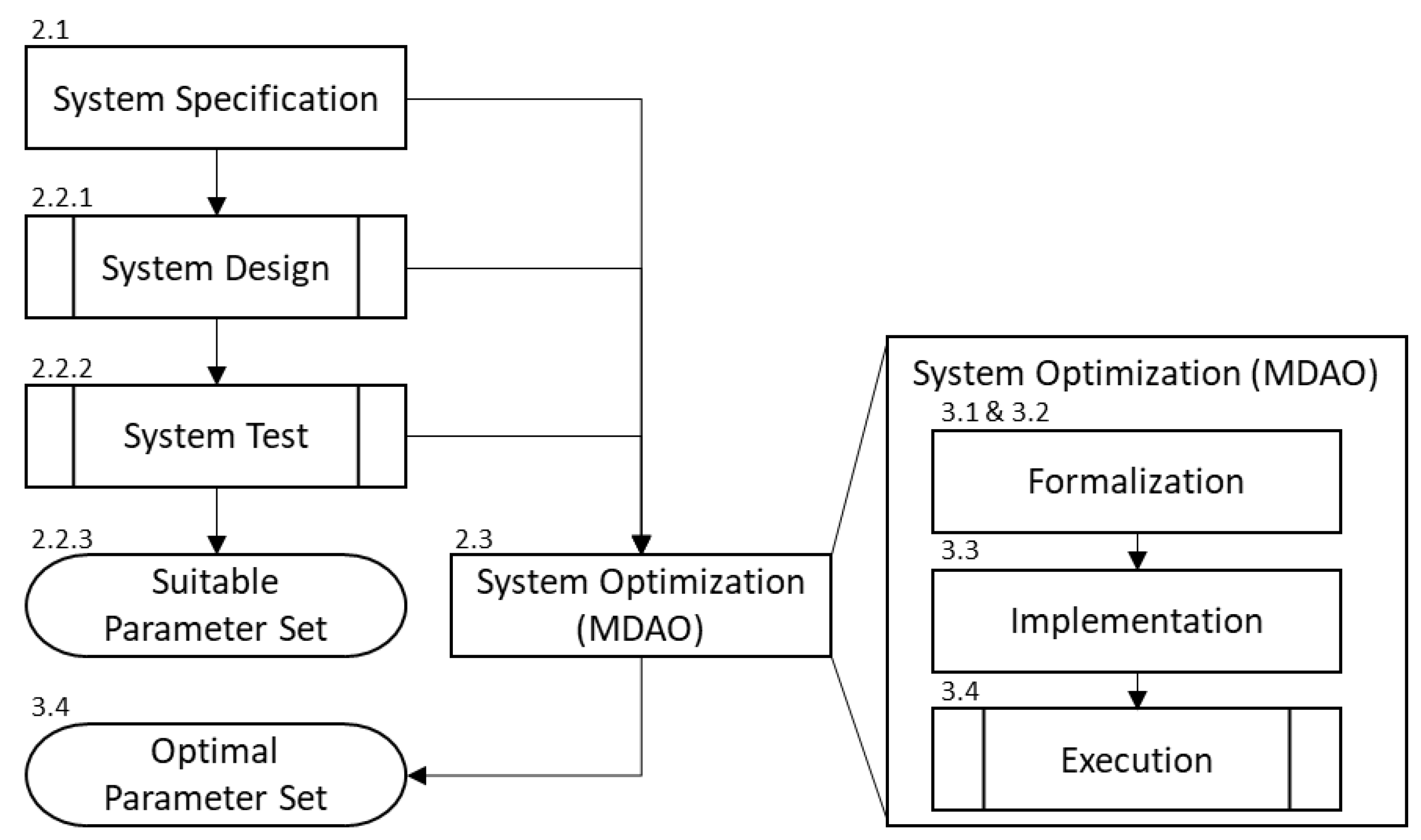
• A novel approach (Section 2) is developed to link MDAO in MBSE system models. The novelty lies in reusing existing development data. For this, data from the system specification and models from design (Section 2.2.1) and test activities (Section 2.2.2) are reused. Utilizing an analogy (Section 2.2.3), design and test activities are mapped to system optimization (Section 2.3). Reusing development data from design and test activities reduces the initial effort of MDAO.
• For the first time, the MDAO problem is formalized in the MBSE system model as an optimization workflow. The purpose is to resolve the MDAO black box behavior and reduce the reconfiguration effort (Section 3.1, Section 3.2 and Section 3.3).

The approach is applied to the optimal design of an electric coolant pump, and exemplary numerical results are presented (Section 3.4).

2. Materials and Methods

The methodological approach of this paper is shown in Figure 2. The main goal is to identify an optimal parameter set for a given system architecture of an MBSE system model by reusing existing development data in model form. The first step is a system specification in which requirements and a suitable system architecture are defined. In the next step of system design, parameters of the system architecture are identified. In the system test, it is verified that the system with the previously identified parameters meets the defined requirements. System design and system tests make use of models. The result of performing system design and test workflows is a suitable set of parameters for the system architecture. Based on the system specification and the models used in system design and test, a system optimization problem (MDAO) is formulated. The execution of the system optimization and solution of the MDAO problem identifies an optimal parameter set for the system architecture. System design, system test, and the executable part of the system optimization are executable workflows.

System Design and System Test are modeled as workflows in the MBSE system model. A workflow is a sequence of executable actions (e.g., implemented models, guidelines, standards) for a specific purpose [27]. A design workflow generates a parameter set that parameterizes the system architecture based on calculation rules from a set of design variables. These parameters describe, for example, geometric dimensions and system behavior. A test workflow is used to test the parameterized system architecture in defined cases and check the fulfillment of requirements. If requirements are not met, the design variables are adjusted, and design and test workflows are executed again.

With increasing system complexity, it is difficult to estimate which design variable changes are suitable for finding a good technical variant or any technical variant. Furthermore, a conflict of objectives can arise that cannot be resolved appropriately by a manual iteration in the design and test workflows. In this case, an optimization workflow is formulated and executed from existing models of the design and test workflows. The result of the optimization workflow is an optimal parameter set of the system architecture. In this paper, we proposed formalizing the optimization workflow by three modeling approaches: workflow architecture, internal behavior, and executable behavior. The main purposes of the formalization are the resolution of the MDAO black box behavior and the provision of a means to parameterize the system architecture with an optimal parameter set. The workflow architecture captures the hierarchical relationships between the workflow elements. In the internal behavior, the black box character of the underlying MDAO of the optimization workflow is resolved by formalizing the utilized models, their interfaces, and execution orders. From this formalization, the MDAO problem is implemented in an external tool. The executable behavior triggers the solution of the MDAO problem from the MBSE system model. The results are fed back to the MBSE system model and provide an optimal parameter set for the system architecture.

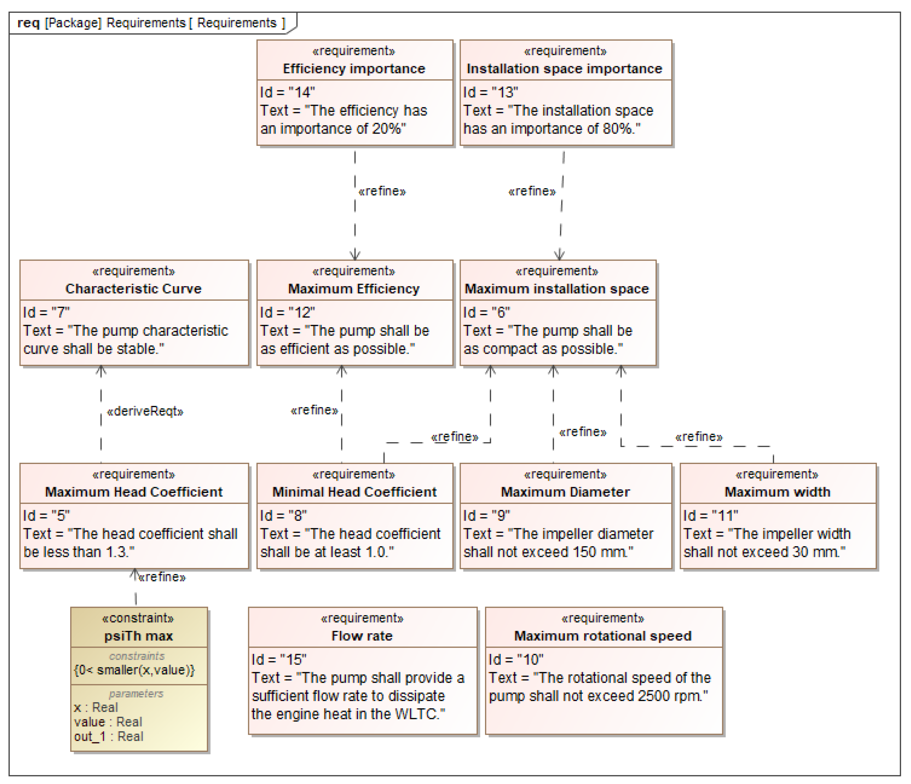
2.1. System Specification

For example, the optimum design of an electric coolant pump in a vehicle is considered regarding the objectives of electric energy consumption and installation space. For this, five design variables are considered: rotational speed, flow rate, and head (i.e., pressure difference between pump intake and outlet) in the best efficiency design point, as well as the impeller vane exit angle and number of impeller blades. The speed of conventional belt-driven coolant pumps is fixed to the speed of the internal combustion engine. This means that the flow rate cannot be supplied as required. The flow rate is therefore adapted by throttling or bypassing, and as a result, energy losses occur. In contrast, electric coolant pumps can provide volume flows as required by adjusting the pump speed, thus helping to reduce energy consumption and ultimately achieve CO₂ targets [28]. The optimal design is discussed in the literature [29,30,31,32].

The main function of an electric coolant pump is to generate a flow rate. To do this, electrical energy is converted to mechanical energy, and this mechanical energy is then applied to the coolant. The amount of electrical energy that can be supplied to the system is controlled to match the provided flow rate to the demand. This relationship is described in Figure 3. The functional architecture of the generate flow rate function is modeled using Koller’s approaches [33]. The described functions represent elementary functions that are realized by principle solutions. In this way, functions and the physical product are linked. The language profile SysML4FMArch was used for the modeling [3]. This approach is particularly suitable because products in the automotive industry are increasingly being developed on a function-oriented basis instead of on a component-oriented basis, as has been the case to date [34].

For linking function and physical product in systems engineering, alternatives exist in the literature, such as the contact and channel approach (C&C-A) [35].

Principle solutions consist of a physical effect that acts in a set of active surfaces consisting of materials. The principle solution for the function apply mechanical energy to fluid is a hydrodynamic pump and shown as an example in Figure 4. The physical effect used in this case is hydrodynamics. The active surface set is formed by an impeller and its pump housing. Multiple parameters describe the active surface set, nine of which ultimately define the physical behavior, i.e., the physical effect of the hydrodynamic pump. For the given parameters and provided interface pressure and speed inputs, the physical effect calculates the acting torque and provided flow rate of the pump. The choice of parameters is therefore decisive for whether and to what extent requirements (e.g., flow rate) are satisfied. The parameter values are determined by an appropriate development process.

2.2. System Design and Test

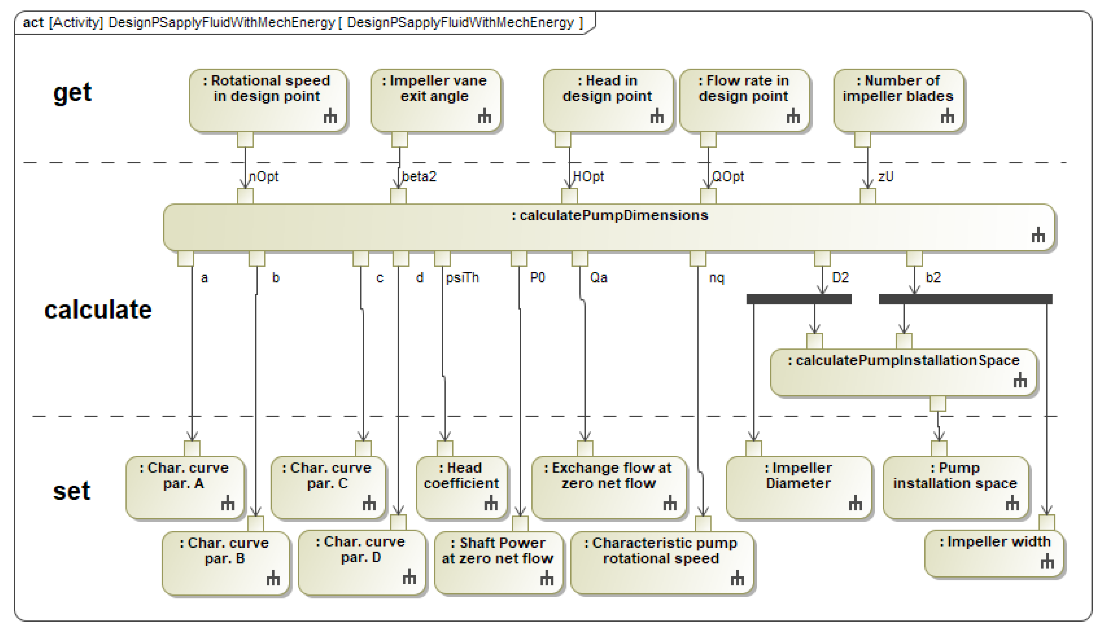
2.2.1. Design Workflow

Design workflows can identify suitable parameter values of the solution architecture [27]. A design workflow model established procedures for design, such as those given in norms, standards, and guidelines in an executable form in the MBSE system model. The design workflow is modeled as an activity diagram for this purpose. The design workflow of a pump impeller is shown as an example in Figure 5. It is divided into three sections: get, calculate and set.

The design of the pump impeller requires the selected values of the design variables to perform calculations. Actions in the get section, therefore, read the associated values from the MBSE system model and make them available for further actions. The following five design variables (cf. get section Figure 5) are set by the systems engineer and read from the MBSE system model:

• Rotational speed $n_{Opt}$, flow rate $Q_{Opt}$ and head $H_{opt}$ in the best efficiency design point indexed as Opt
• Impeller vane exit angle ${\beta }_2$
• Number of impeller blades $z_U$

The calculate section contains actions that use methods to calculate parameter values of the principle solution. These actions can represent simple analytical relationships (as in calculatePumpInstallationSpace) or trigger extensive calculations stored in external tools (as in calculatePumpDimensions). Although the design of the pump is based on principles of hydrodynamics, the calculation in calculatePumpDimensions differs from the model of the physical effect in Figure 4. The physical effect models the in- (rotational speed and pressure difference) and output (torque and flow rate) behavior of the pump. In contrast, the design workflow determines the necessary parameters of the physical effect. After the calculations in the workflow, the parameter values must be transferred back to the MBSE system model. The values can be used by further calculations or checked for requirement satisfaction. The following eleven parameter values (cf. set section in Figure 5) are calculated from the five design variables and written back to the MBSE system model:

• Parameter values of the pump characteristic curve $a, b, c, d$
• Head coefficient ${\psi }_{Th}$
• Impeller diameter $D_2$ and width $b_2$
• Pump installation space $V_{Pump}$
• Shaft power at zero net flow rate $P_0$
• Exchange flow rate at zero net flow rate $Q_a$
• Characteristic pump rotational speed $n_q$

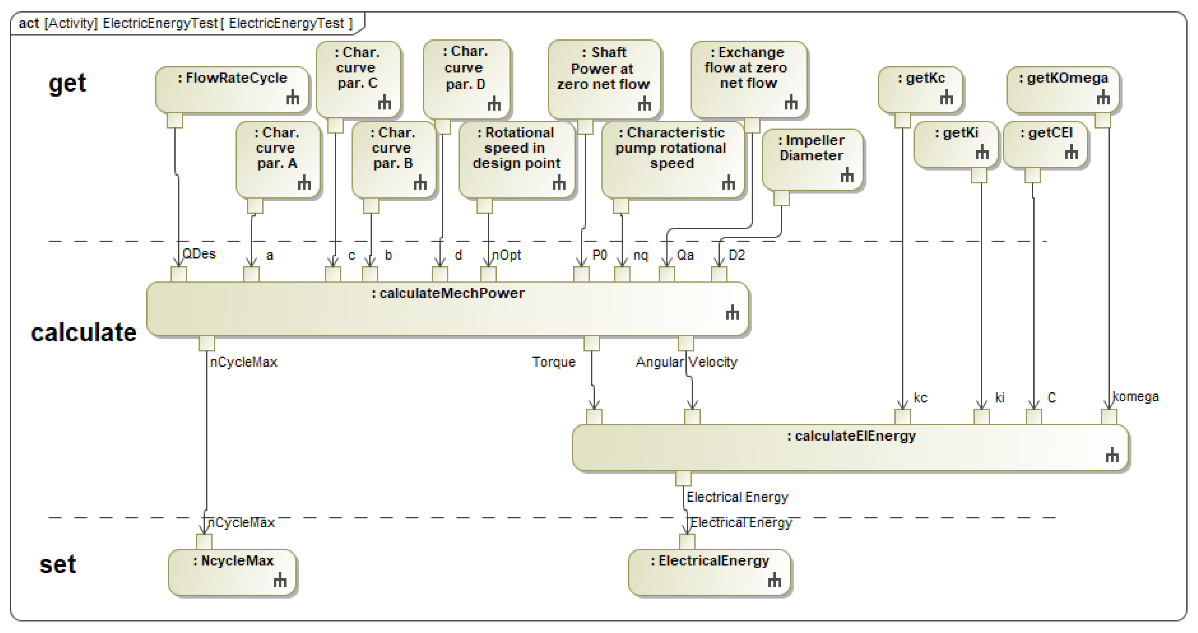
2.2.2. Test Workflow

Design workflows determine parameter values of principle solutions for defined design scenarios. With this determined parameter value set, a technical variant is created. In contrast to design workflows, test workflows check whether the developed technical variant meets all requirements. This is necessary because not all boundary conditions and requirements are generally considered in the design. For example, hydrodynamic pumps are designed for the best efficiency point consisting of rotational speed, flow rate, and head (pressure difference between pump intake and output). During operation, however, the speed is varied to adapt the flow rate to the heat dissipation requirements in the cooling circuit. The pump is then operated off the best efficiency point. The resulting energy consumption in operation is, therefore, a quantity that is not captured by the design workflow but calculated in the test workflow. Identifying the most suitable design point considering the later operation is an engineering challenge.

In this paper, the exemplary requirements for the electric coolant pump, as shown in Figure 6 will be considered for the test workflow.

From the higher-level requirements for high efficiency, low installation space, and stable operation, a range of values are derived for the head coefficient. The head coefficient is a characteristic value calculated from the physical quantities of a pump and characterizes its operating behavior [36]. The head coefficient should be as high as possible for compact and efficient pumps [37]. A lower bound of ${\psi }_{Th,min}=1.0$ is therefore selected. However, a head coefficient that is too high can lead to unstable flow rate behavior and vibration excitations in the cooling circuit [38]. The value of the head coefficient is therefore limited to ${\psi }_{Th,max}=1.3$ using a practical value according to [39]. The installation space requirement is further refined in maximum impeller diameter and width. These limits depend on the application and are here set to $D_{2,max}=150 \mathrm{mm}$ and $b_{2,max}=30 \mathrm{mm}$. Additionally, the pump shall be operated at a maximum speed of $n_{max}=2500\frac{1}{min}$ for noise and material strength reasons. Further requirements weigh the importance of installation space and efficiency of the pump. The so defined weights can be used to compare different technical variants. The WLTC is used as the design cycle. The pump must provide enough flow rate to dissipate the heat generated by the engine in the cycle. The requirements are checked utilizing constraint elements in the MBSE system model. For brevity, only one such element is shown in Figure 6 for the upper limit of the head coefficient. These constraints are later reused identically in MDAO.

A test workflow is modeled similarly to the design workflow in an activity diagram (Figure 7). It consists of the sections get, calculate, and set. In the present example, two successive tests in the form of simulations are performed: A mechanical (calculateMechPower) and an electrical (calculateElEnergy) performance test. The implementations of calculateMechPower and calculateElEnergy are described in detail in Section 3.4. For the mechanical performance test, the previously determined pump impeller design variable values and the flow rate cycle are loaded using get actions. The mechanical performance test determines the time histories of the mechanical pump torque and rotational speed, as well as the maximum required pump speed $n_{cycle,max}$ in the flow rate cycle. For the electrical performance test, parameter values of the electric motor are loaded by means of get actions. This test receives the additional time histories of torque and speed and calculates the consumed electrical energy $E_{El}$ in the flow rate cycle. The design of the electric motor is not considered in this paper. Therefore, the parameter values of the electric motor remain constant. After the electrical performance test, the results of the test workflow are transferred back to the MBSE system model using set actions, that is, the parameter values of $n_{cycle,max}$ and $E_{El}$. There, it is checked to see whether the specified requirements are met. For example, the permitted maximum speed is compared to the calculated quantitative value. The consumption of electrical energy is not further specified in the requirements; thus, it could be compared to benchmarks and technical variants. If requirements are not met, a new and suitable technical variant must be found.

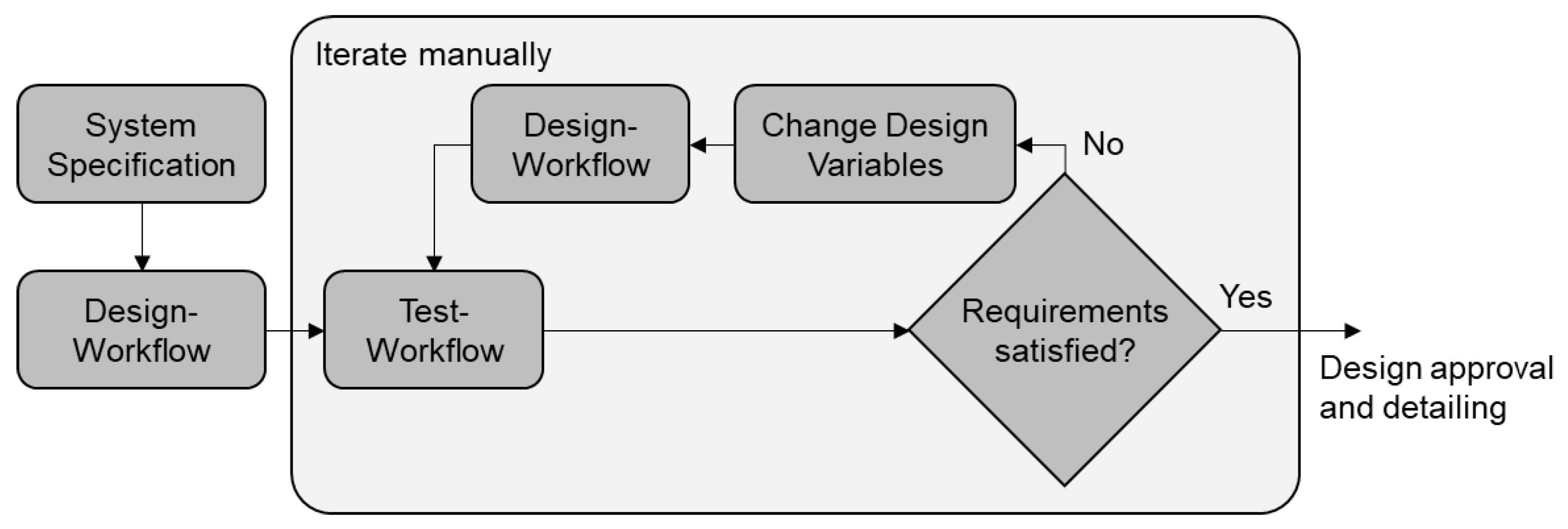
2.2.3. Design and Test Process

The process of executing the design and test workflows is shown in Figure 8. This manual process is characterized by decisions at each stage based on intuition or experience [40].

First, in Figure 8, the system is specified in the MBSE system model. The system specification includes the collection and definition of requirements and the derivation of a suitable functional and solution architecture. From this, simulation models are derived and linked in design and test workflows. The design workflow uses these models and other calculations (norms, standards, and guidelines) to determine the parameters of the solution architecture. In the test workflow, parameter values are calculated and checked for requirement satisfaction. If requirements are not met, the design variables are changed, and the design and test workflows are executed again. If the requirements are met, the design can be approved and detailed. There may arise the case that no technical variant can fulfill the requirements. Then requirements can be relaxed, or they can be returned to a previous development phase to adapt the system architecture. These two cases are not considered in this paper.

In the case of the electric coolant pump, there are any number of technical variants that meet the exemplary requirements (Figure 6). However, during the design and test activities, the pump installation space and electric energy consumption arise as conflicting objectives. This means that the requirements for the highest efficiency and smallest installation space are met to varying degrees by different technical variants.

With increasing system complexity, it is difficult to estimate which design variable changes are suitable for finding a good variant or any variant at all. Furthermore, it is unclear which design variables are particularly suitable for responding to requirement changes.

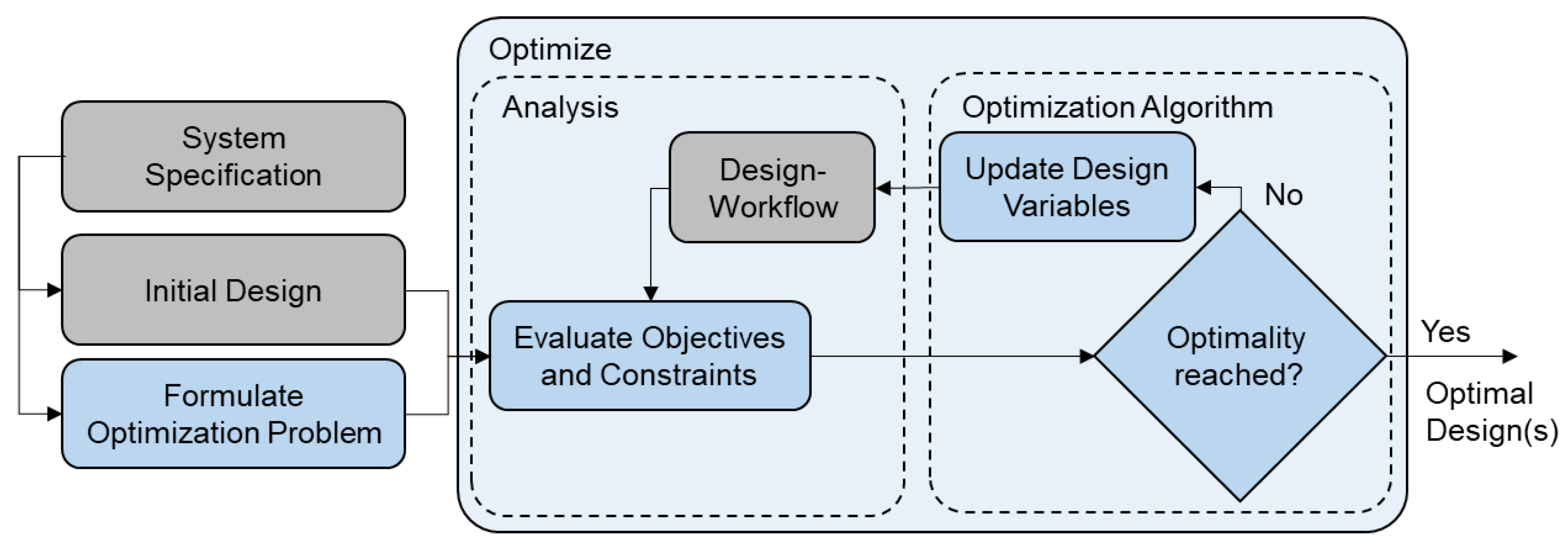
2.3. System Optimization

To avoid a costly manual iteration, an analogy of the design and test process with a general MDAO process (Figure 9) is considered. Similar to the manual iteration, the process starts with a system specification. In addition, the optimization problem must be formulated. If the optimization algorithm needs starting values, an initial system design is provided. The optimization itself is divided into two parts: analysis and the optimization algorithm. In the analysis, objective and constraint functions are evaluated. In the manual iteration, this corresponds to the execution of the test workflow as well as the requirement verification. In the case of optimization, quantifiable requirements are formulated as constraint functions and evaluated automatically by the optimization algorithm. The contents of the analysis can be selected freely. If the execution of the test workflow requires a previous execution of the design workflow, it can be placed in the analysis. The optimization algorithm receives the evaluated objective and constraint function values and uses defined criteria to decide whether optimality has been achieved. If not, the design variables are updated and supplied to the analysis. This iteration is performed until optimality is reached. If optimality is reached, the optimization outputs one or more optimal technical system variants. If several optimal technical system variants are available (e.g., in the case of multiobjective optimization), a selection of the best tradeoff must then be made by the system engineer based on preferences [41].

Compared to the manual iteration (Figure 8), the variation of design variables is performed systematically. Requirement changes can be met by reformulating the constraints.

To make use of the MDAO process in the MBSE system model an optimization workflow is proposed.

3. Results: Optimization Workflow

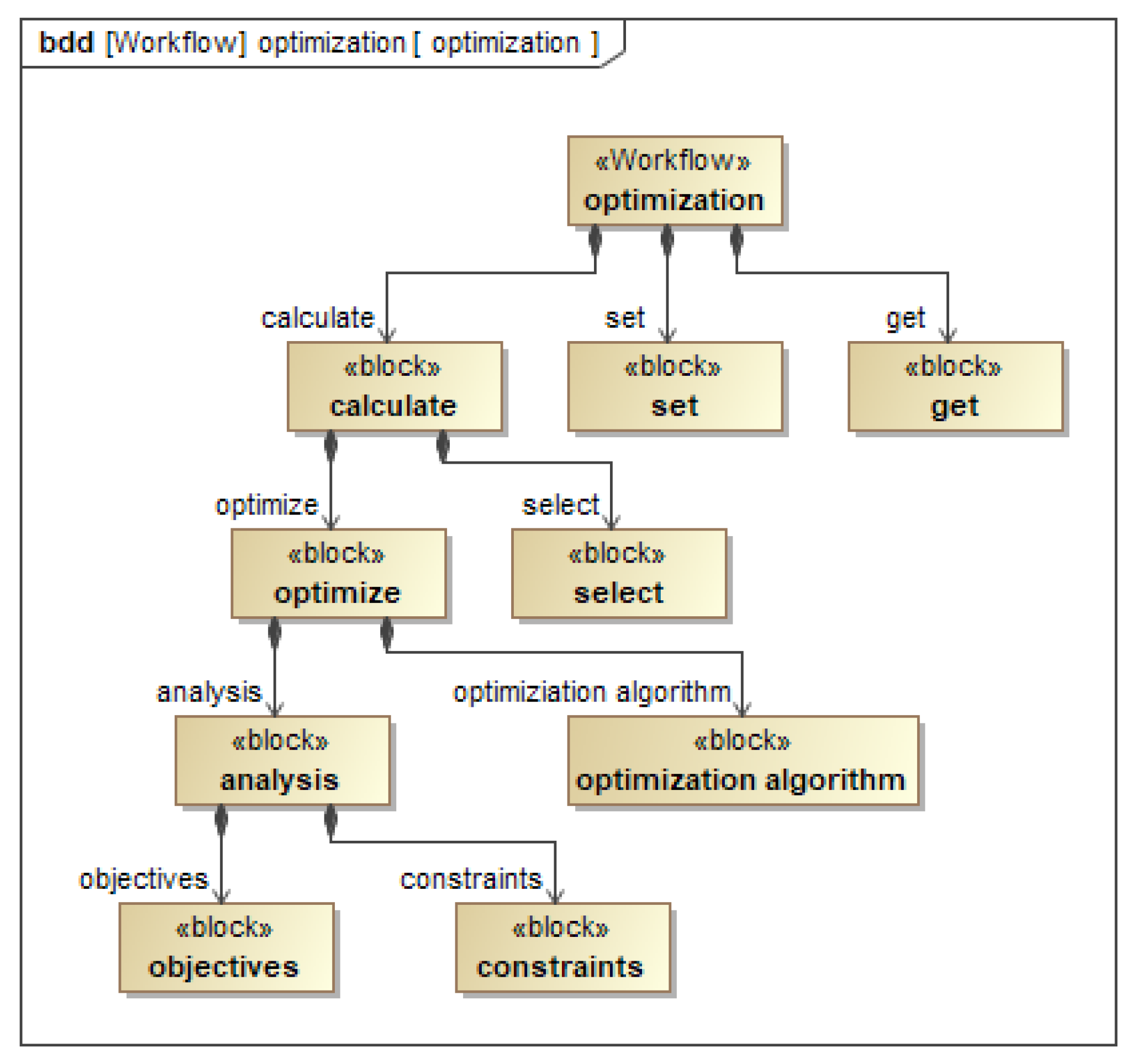
3.1. Workflow Architecture

The architecture of the optimization workflow describes the hierarchical relationships of its elements and is, therefore, part of the formalization process in Figure 2. The workflow architecture is modeled as a block definition diagram (bdd) and is shown in Figure 10. Similar to the design and test workflows, the optimization workflow consists of the sections get, calculate and set. Calculate consists of the parts optimize and select. The block select is used to select the most suitable tradeoff if multiple optimal variants are available. Optimize consists of an analysis and an optimization algorithm (corresponding Figure 9). [In the analysis, objectives, and constraints (implemented as functions) are evaluated. The optimization algorithm performs the optimization task.

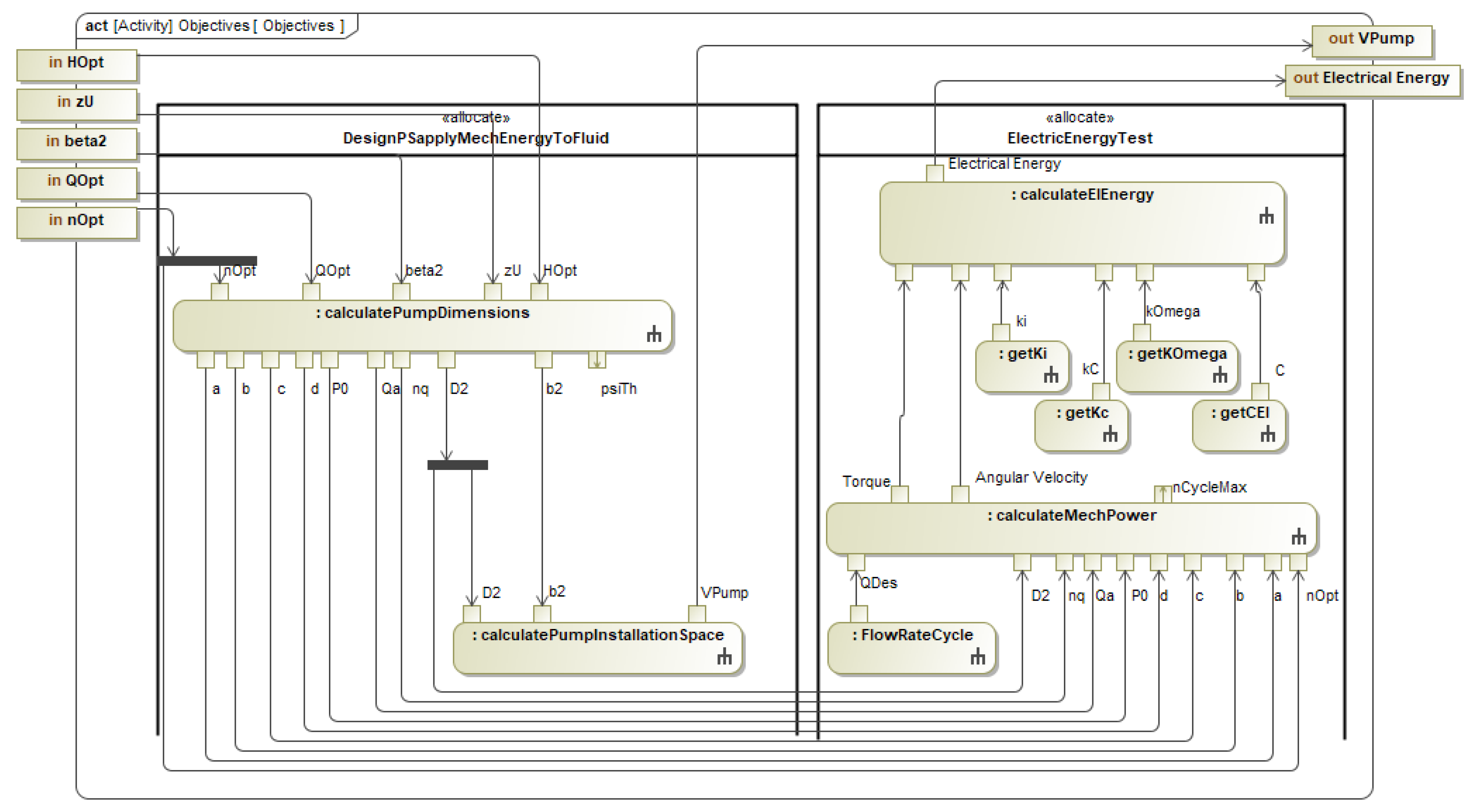
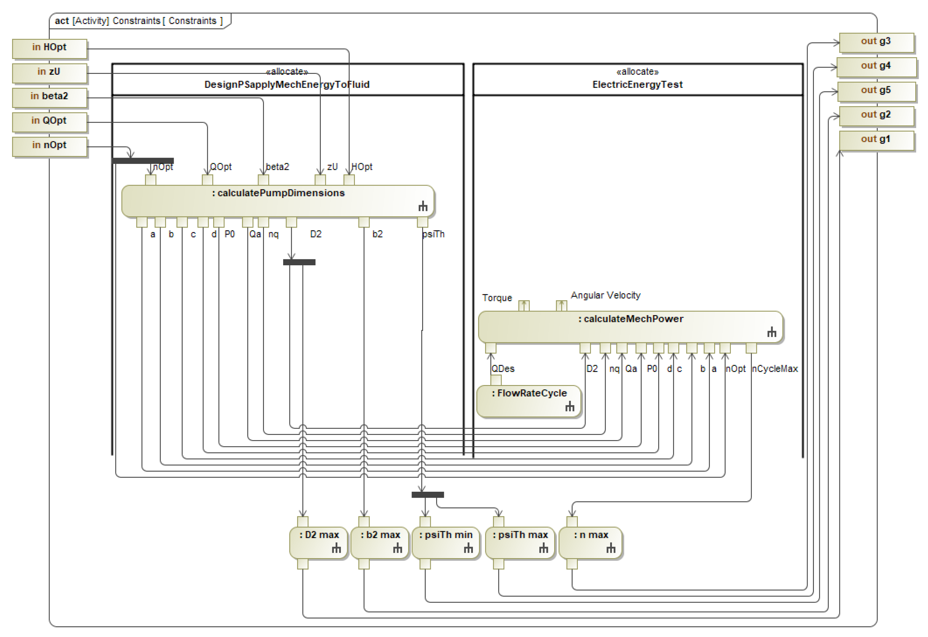
3.2. Internal Behavior

The internal behavior describes the sequence and execution order of the optimization workflow elements. It includes the definition of used models, the exchanged parameters at interfaces, and considered system requirements in MDAO. It is also the workflow architecture part of the formalization process in Figure 2. The internal behavior of the optimize block (Figure 11) describes the exchange of design variables as well as evaluated objective functions $f$ and constraint functions $g$ between the optimization algorithm and the analysis (cf. Figure 9).

The internal behavior of the objectives block is shown in Figure 12. In this depiction, the design variables and the objectives are defined. For example, all design variables of the design workflow were adopted (cf. Figure 5). The objectives were defined based on the identified conflict of objectives in the manual iteration (pump installation space and electrical energy consumption). Model elements of the design (calculatePumpDimensions, calculatePumpInstallationSpace) and test (calculateMechPower, calculateElEnergy) workflows were reused in the description of the internal behavior (cf. Figure 5 and Figure 7).

The activity diagram for calculating the constraints is given in Figure 13. On the input side, the calculation receives the current values of the design variables. On the output side, the values of the constraint functions ($g_1\dots g_5$) are returned. The values of the constraints result in the execution of actions of the design (calculatePumpDimensions) and test (calculateMechPower) workflows. The actions for checking the requirements use the same constraints that refine the requirements (cf. Figure 6).

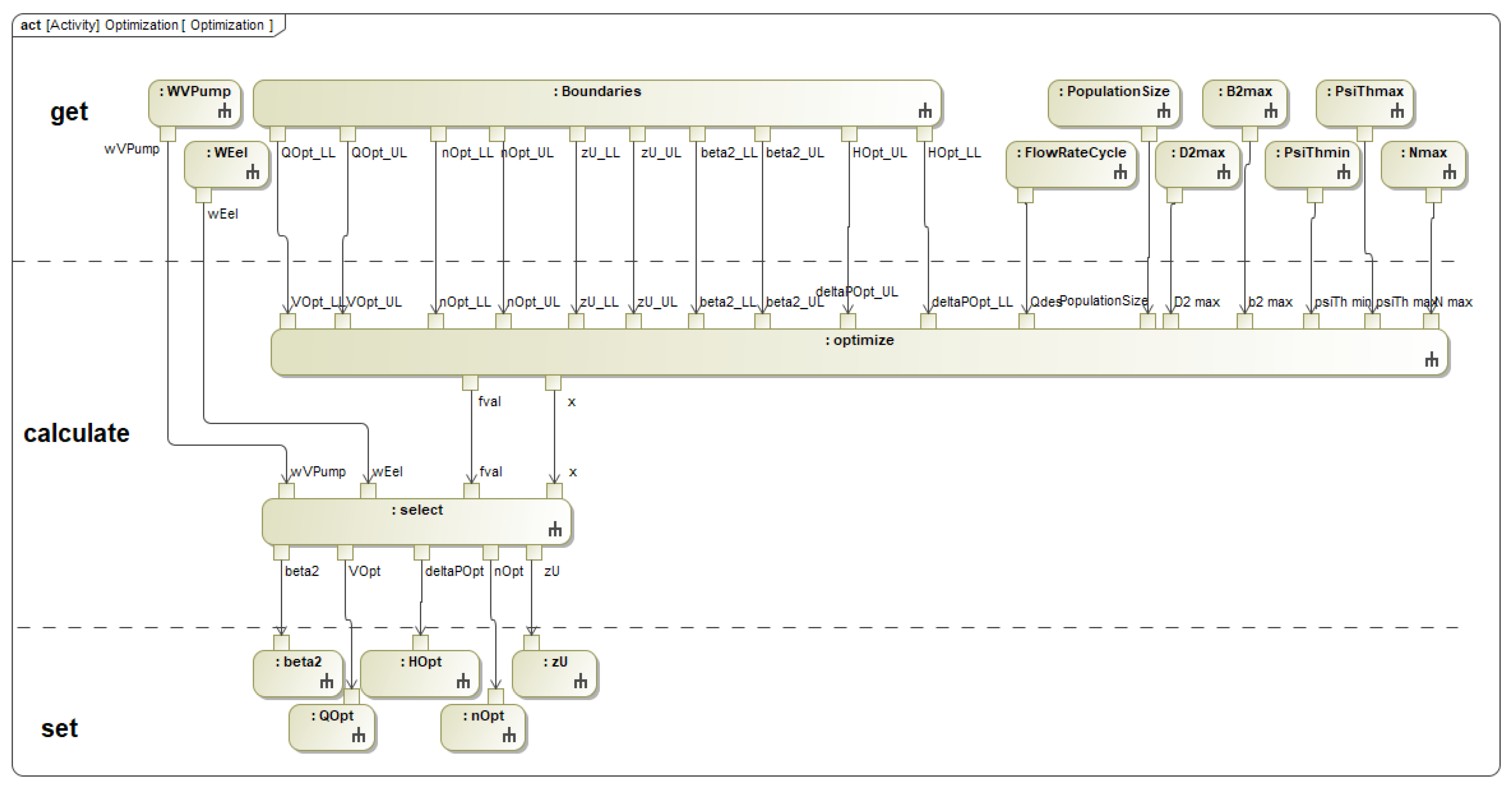
3.3. Executable Behavior

The executable behavior of the optimization workflow triggers the solution of the MDAO problem in an external tool. The executable behavior of the optimization workflow is modeled in an activity diagram (Figure 14). In the get section, necessary parameters such as the flow rate cycle are read out from the MBSE system model and provided to the calculate section. The upper and lower variation bounds of the design variables are loaded collectively in the Boundaries action. These limits can be based on empirical values or physical limits. Furthermore, the parameter values of the requirements (B2max, D2max, PsiThmax, PsiThmin, Nmax) are loaded, and thus the constraints of the optimization are parameterized. In this paper, a genetic algorithm is used for optimization. Therefore, a hyperparameter of the population size is loaded. The two weights, WVPump and WEel, are used to select the technical variant with the best tradeoff between installation space and electrical energy consumption from the resulting pareto front. The numerical values of the weights are defined in the requirements (cf. Figure 6).

The calculate section consists of an optimize and a select action. Optimize calculates a matrix of non-dominating technical variants (pareto front) by solving the optimization problem. The optimize action is implemented in an external tool reusing the predefined models in the internal behavior description. This corresponds to the implementation process in Figure 2. The select action weights the technical variants on the pareto front to determine the best tradeoff. In the set section, the design variable values of the selected tradeoff are transferred to the MBSE system model to be checked for requirement satisfaction.

In the MBSE system model, the optimize action exhibits black box behavior, which is resolved with the help of the workflow architecture (Figure 10) and internal behavior (Figure 11 and Figure 12).

Changes in the requirement values (maximum diameter, flow rate cycle, etc.) can directly be considered in the optimization execution. For this purpose, the values linked to the requirements are automatically transferred to the optimize action by the corresponding actions (D2max, FlowRateCycle, etc.) in Figure 14. Likewise, the variation limits of the design variables can be changed via the defined interfaces. This reduces the reconfiguration effort of the MDAO problem.

New requirements, other objectives, and design variables, as well as new calculation steps, represent changes to the internal behavior of the optimization workflow. These changes must be specified in the internal behavior by the systems engineer and, on this basis, reimplemented in new executable behavior.

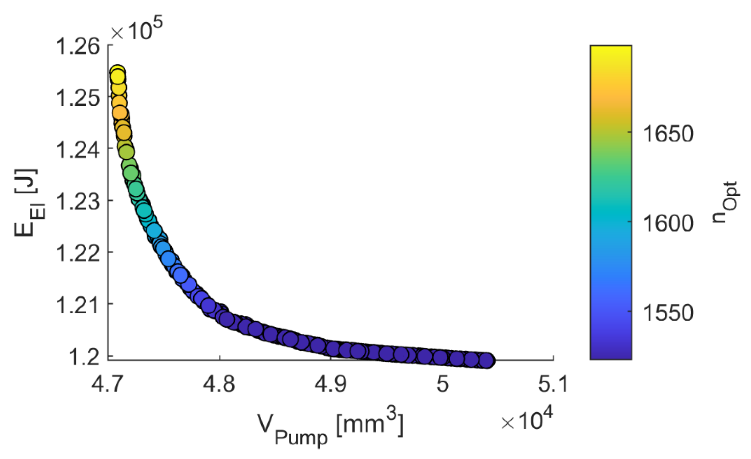
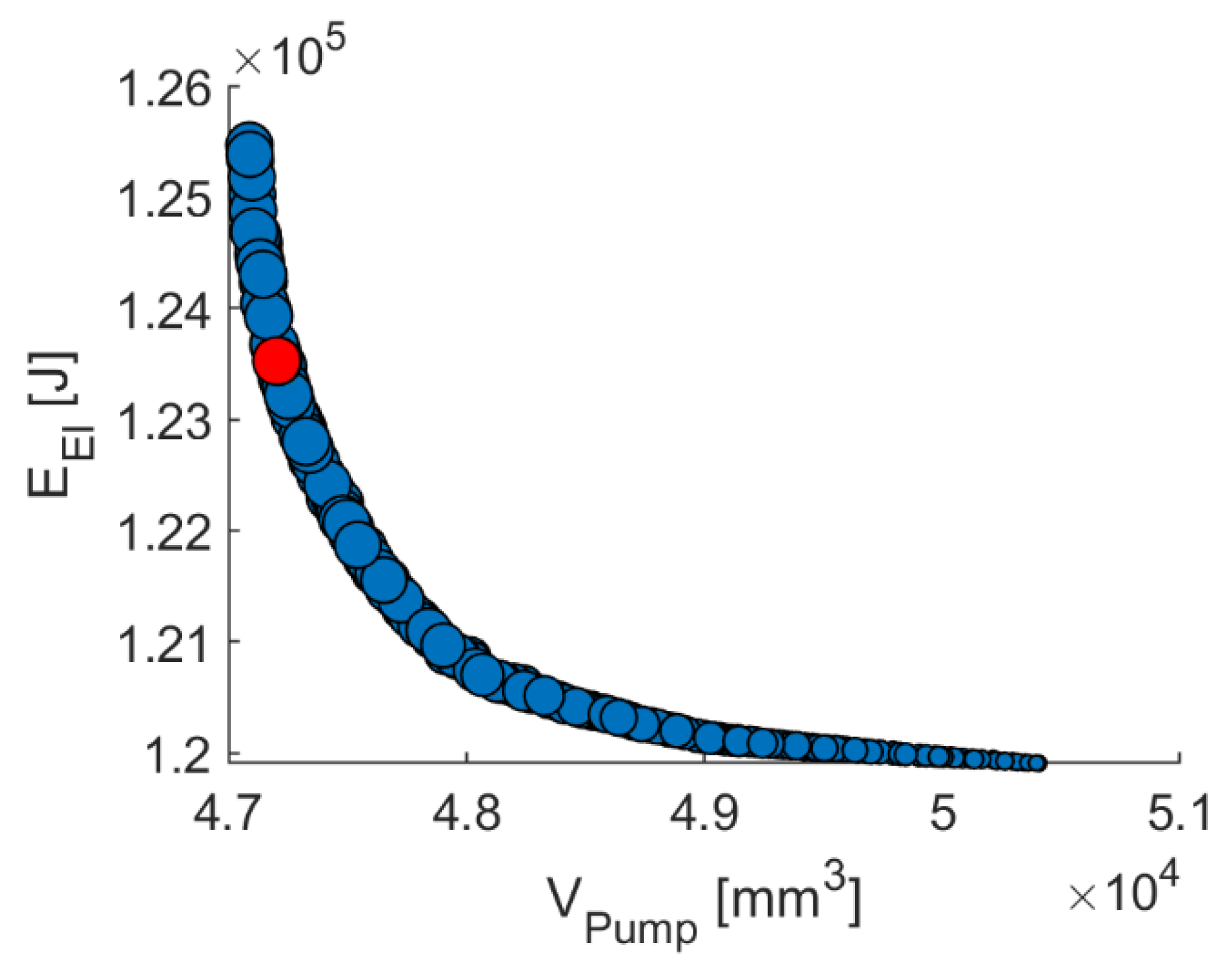
3.4. Numerical Results

Executing the optimization workflow (cf. Figure 2) produces numerical results, which are presented below. The visualization of the resulting MDAO problem is given as an extended design structure matrix (XDSM) in Figure 15. A Matlab implementation of the genetic algorithm NSGA-II is used as the optimization algorithm, which can handle discrete and real-valued design variables and consider constraints and multiple objectives. The algorithm is suitable for optimizing various engineering problems ranging from gearboxes [42,43] to wind farms [44,45].

A pump is designed based on five design variables. With this design, a mechanical shaft power must be provided to the pump for a given flow rate cycle. The connected electrical motor provides this shaft power and consumes an amount of electrical energy in the process. Four variables (head coefficient ${\psi }_{Th}$, maximum rotational speed $n_{max}$, maximum impeller width $b_2$ and diameter $D_2$) are constrained by five nonlinear constraints ($g$), which are given by the system requirements (Figure 6). The installation space of the pump $V_{Pump}$ ($f_1$) and the required amount of electrical energy $E_{El}$ ($f_2$) are objectives.

The design of the electric coolant pump is based on the procedure in [39]. The design determines the flow characteristics (described by the pump characteristic curve), efficiency, and spatial dimensions of the pump. In the design process under consideration, five design variables are available for this purpose: pump rotational speed $n_{Opt}$, flow rate $Q_{Opt}$ and head $H_{opt}$ in the best efficiency point as well as impeller vane exit angle ${\beta }_2$ and number of impeller blades $z_U$. The mathematical optimization problem is formulated as follows (Equation (1)):

$$\begin{gathered} \mathrm{minimize}f\left(x\right)=\left(V_{Pump},E_{El}\right) \\ \mathrm{by}\mathrm{varying}x=\left(n_{Opt},Q_{Opt},H_{opt},{\beta }_2,z_U\right) \\ \mathrm{subject}\mathrm{to}{g}_1\left(x\right)=D_2-D_{2,max}<0 \\ {g}_2\left(x\right)=b_2-b_{2,max}<0 \\ {g}_3\left(x\right)=n_{cycle,max}-n_{max}<0 \\ {g}_4\left(x\right)={\psi }_{Th}-{\psi }_{Th,max}<0 \\ {g}_5\left(x\right)={\psi }_{Th,min}-{\psi }_{Th}<0 \end{gathered}$$

(1)

The pump characteristic curve (Equation (2)) defines the head $H$ and flow rate $Q$ behavior of the pump at constant rotational speed. The coefficients $a$, $b$, $c,$ and $d$ are functions of ${\psi }_{Th}$, $Q_{Opt}$, $H_{Opt}$ and $n_q$ and determined using the design workflow.

$$H=a\cdot Q^3+b\cdot Q^2+c\cdot Q+d$$

(2)

The system characteristic curve describes the head and flow rate behavior of the cooling circuit. An operating point consisting of head and flow rate is set as the intersection of the pump characteristic curve and the system characteristic curve. In the considered pump application, the necessary flow rate depends on the amount of heat to be dissipated by the cooling circuit. The operating point is therefore changed by adjusting the pump rotational speed. This operating point shift is modeled by scaling the pump characteristic curve according to the affinity laws in Equations (3) and (4). Index I indicates the unscaled, and index II the scaled operating point. The system characteristic curve remains constant.

$$\frac{Q_{II}}{Q_I}=\left(\frac{n_{II}}{n_I}\right)$$

(3)

$$\frac{H_{II}}{H_I}={\left(\frac{n_{II}}{n_I}\right)}^2$$

(4)

These relationships are shown in Figure 16. Changing the pump speed to adjust the flow rate to the demand generally results in a decrease in pump efficiency $\eta$.

In this paper, the coolant flow rate requirement of an internal combustion engine for a mid-size vehicle in the Worldwide harmonized Light-duty vehicles Test Cycle (WLTC) is considered. In the driving cycle, the engine power and, therefore, heat generation varies over time. This results in a varying coolant flow rate. Due to the varying flow rate, the pump is not operated continuously at its best efficiency point. The resulting operating range of the pump in the WLTC is given in

Table 1. Maximum and minimum flow rate and head values in the WLTC.

Variable	$\mathit{Q}$	$\mathit{H}$
Lower limit	30 $\frac{l}{\min }$	4.9 $\mathrm{kPa}$
Upper limit	363.4 $\frac{l}{\min }$	30 $\mathrm{kPa}$

. For efficient operation, it is crucial to appropriately select the best efficiency point of the pump along with the number of impeller blades and impeller vane exit angle.

The installation space of the pump impeller ($f_1$ in Figure 15) is calculated from its diameter and width, which are provided by the pump dimensioning. The pump dimensioning provides a total of nine quantities for calculating the mechanical shaft power (Figure 15).

The mechanical shaft power of the pump $P_{shaft}$ is composed of four components (Equation (5)). $P_h$ is the hydrodynamic power and takes into account power for conveying the net flow rate and the occurring gap loss flows. The disk friction power $P_R$ includes all losses caused by fluid friction on rotating components wetted by the pumped coolant. The mechanical power $P_m$ includes all losses that occur at the bearings and dynamic seals. Exchange losses $P_a$ occur mainly when the pump is operated at a significantly lower flow rate than the best efficiency point. The pump is then in partial load operation, characterized by turbulence behind the pump impeller. Backflows occur, which act back on the impeller and are captured in the additional power $P_a$.

$$P_{shaft}=P_h+P_R+P_m+P_a$$

(5)

The losses of the electric motor $P_{el, loss}$ are described by the analytical approximate Equation (6) [46]. The torque $T$ and the angular velocity $\omega$ correspond to the operating point of the electric motor and are determined by the calculation step of the mechanical power demand (Figure 15). The parameters $k_c$, $k_i$, $k_{\omega },$ and $C$ were determined by numerical fitting of the efficiency map of the known and unvaried electric motor.

$$P_{el,loss}=k_c\cdot T^2+k_i\cdot \omega +k_{\omega }\cdot {\omega }^3+C$$

(6)

The consumption of electrical energy ($f_2$ in Figure 15) is determined by time integration of the mechanical power and electrical power loss (Equation (7)).

$$E_{el}=\int P_{shaft}+P_{el,loss}dt$$

(7)

The design variables are varied within the limits specified in

Table 2. Variation limits of the design variables.

Design Variable	${\mathit{n}}_{\mathit{O}\mathit{p}\mathit{t}}$	${\mathit{Q}}_{\mathit{O}\mathit{p}\mathit{t}}$	${\mathit{H}}_{\mathit{O}\mathit{p}\mathit{t}}$	${\mathit{\beta }}_2$	${\mathit{z}}_{\mathit{U}}$
Lower limit	1500 $\frac{1}{\min }$	60 $\frac{l}{\min }$	12 $\mathrm{kPa}$	25°	7
Upper limit	3000 $\frac{1}{\min }$	600 $\frac{l}{\min }$	30 $\mathrm{kPa}$	35°	9

. The limits of $n_{Opt}$, $Q_{Opt}$ and $H_{opt}$ are selected based on trial executions. The limits of the number of impeller blades and impeller vane exit angle ${\beta }_2$ are selected based on empirical values according to the literature [39].

In this paper, we present the results of the multiobjective optimization using pareto fronts. A pareto front contains all variants which do not dominate each other with respect to their objectives. If two variants are compared on the pareto front, one variant will be better in one objective and worse in the other [40].

The pareto front of the optimization problem regarding the constraints is shown in Figure 17. It can be seen that spatially compact pumps have a higher energy consumption. Efficient pumps, on the other hand, take up a larger installation space. The influence of the design parameter $n_{Opt}$ of the best efficiency point is shown as an example. Here, higher rotational speeds in the best efficiency point lead to more compact but less efficient pumps.

In this paper, the best tradeoff (cf. select in Figure 14) is selected by a weighted rating of the two objectives (Equation (8)). For this purpose, the objective values $E_{El}$ and $V_{Pump}$ of each technical variant on the pareto front are first scored. An objective with the lowest value is assigned the score $S$ of 10, an objective with the highest value is assigned the score $S$ of 1. Objective values in between are assigned a linear interpolated score between 1 and 10. A variant on the pareto front is thus assigned two scores between 1 and 10. By specifying two weights $w$, both variant scores are reduced to one. The two weights describe the importance of the objectives to the systems engineer. The technical variant with the highest total score $S_{tot}$ corresponds to the most preferred variant. A similar approach is used in [47].

$$S_{tot}=w_{E_{El}}\cdot S_{E_{El}}+w_{V_{Pump}}\cdot S_{V_{Pump}}$$

(8)

The selection of the most suitable variant is shown as an example in Figure 18. The pump installation space was weighted at 80% ($w_{V_{Pump}}=0.8$) and the energy consumption of 20% ($w_{E_{El}}=0.2$) importance (cf. Figure 6).

The values of the selected technical variant are summarized in

Table 3. Numerical values of the selected technical variant in Figure 18.

Design Variables					Objectives
$n_{Opt}$	$Q_{Opt}$	$H_{opt}$	${\beta }_2$	$z_U$	$E_{El}$	$V_{Pump}$
1635 $\frac{1}{\min }$	150 $\frac{\mathrm{l}}{\min }$	12.11 $\mathrm{kPa}$	34.95°	9	123.53 $\mathrm{kJ}$	47203 ${\mathrm{mm}}^3$

. It represents the best variant in the context of system preference [41]. The limits of the variables $n_{Opt}$ and $Q_{Opt}$ are not exploited by the optimization algorithm. For the variables $H_{opt}$, ${\beta }_2$ and $z_U$ it can be seen that the variation limits are reached.

In principle, other decision-making techniques are also applicable. In the literature, FUZZY, LINMAP [48], and TOPSIS [49] are used, among others.

The results from Table 3 are transferred to the MBSE system model and represent an optimal set of parameters of the system architecture (cf. Figure 2).

4. Discussion

The developed approach for linking MDAO with an MBSE system model enables extending the analytical possibilities in MBSE. Large areas of the design variable and the resulting solution space can be explored. As a result, technical variants with the best objectives are identified, and conflicting objectives are resolved with an appropriate tradeoff. The formal description of the MDAO problem in the MBSE system model resolves its black box behavior. Necessary changes in case of new requirements or new available models become transparent, which reduces the reconfiguration effort. If a conflict of objectives is identified based on an existing design and test workflows, the presented approach can be used to formulate an MDAO problem. By reusing models from existing design and test workflows, the initial implementation effort of the MDAO problem is reduced. The formalization of MDAO is carried out employing architecture and internal behavior. These descriptions are transferred to the executable behavior of the workflow, which triggers the execution and solution of the MDAO problem.

Limitations

The transfer of the internal behavior to the executable behavior is done manually at the current time. For the purpose of automatability, a model-to-model transformation of the internal behavior into the executable behavior should be investigated in future work. Additionally, the get and set functions must be implemented manually for each parameter. One solution might be combining multiple get or set functions into one overarching function, as presented in Figure 14. However, this reduces flexibility.

The developed approach was only applied to one MDAO architecture (Figure 15). In the future, its usefulness for other MDAO architectures must be examined. Although the approach can be used in the early stages of development, it assumes that models and workflows are already in place and that a conflict of objectives has been identified. This limits the applicability for deviating boundary conditions. Another limitation of the approach is that MDAO, which considers many parameters, would lead to crowded acitvity diagrams.

5. Related Work

Chaudemar et al. conduct a literature review on the joint use of MBSE and MDAO in the early stages of development [26]. They come to three conclusions: First, there is a lack of confidence that the MDAO problem correctly represents the MBSE system model. Second, the MDAO formulation takes a non-negligible amount of time. At the same time, necessary information is already available in the MBSE system model. Third, MDAO solutions are rarely implemented in the MBSE system model. As reasons, the lack of expressiveness of the MBSE languages and high manual effort are indicated.

Aiello et al. [50] link MDAO and MBSE using the three branches of approach, type, and tool for refining requirements. Thus MDAO is to be used already in the early phases of the requirement formulation. The approach stands for the fact that the MBSE triggers the MDAO execution and the MDAO results enrich the MBSE system model. The type describes a coupling of language and methodical level. On the language level, the description in the MBSE system model is extended by new stereotypes for requirements used for the MDAO formulation (e.g., solver, model accuracy, etc.). Methodically, five steps are proposed to read out these requirements from the MBSE system model and enrich them through MDAO. Papyrus and OpenMDAO are used as tools. The use case is the dimensioning of a drone battery. Reuse of models is not addressed, and the MDAO problem remains a black box for the system engineer. A further work [51] focuses on the refinement of requirements in MBSE by linking them to MDAO. For this purpose, tool interfaces between TTool, OpenMDAO, and UPPAAL-SMC are implemented.

Jeyaraj et al. [52] describe a framework for the joint use of MBSE and MDAO. The MBSE system model contains all the system specification information. MDAO is used to evaluate individual architectures. In the presented example, the MBSE system specification is enriched with MDAO input parameters, and these parameters are extracted and finally evaluated in MDAO. Finally, the MDAO results are fed back into the MBSE system model. The procedure is demonstrated in an aircraft application. The MDAO problem remains a black box in the MBSE system model.

Ciampa et al. [24] describe a linking of MBSE and MDAO using an architectural framework. In this context, the concept of a development system and a system of interest (SoI) is introduced. A development system is one of the supporting systems (simulation, MDAO, etc.) for the development of the SoI in different phases. It is proposed to use MBSE for the development of MDAO systems and thus accelerate the development of SoI. The MDAO system is formally described in structure and behavior by an MDAO system architecture. The MDAO system architecture is developed using an architectural framework consisting of ontology (nomenclature and terminology) and viewpoints (organizational, architectural, lifecycle, process, requirements). In this way, the so-called upstream engineering phases (system identification, specification, architecting), which are formalized by the MBSE, are linked to the downstream engineering phases (system synthesis and exploration), including MDAO. The definition of MDAO as an individual system establishes a vertical integration into the development of complex systems. So far, only high-level elements of this MBSE-driven approach to developing MDAO systems have been published. The reuse of existing development data and models of the system of interest was not described. It is not addressed how MDAO is executed and how the parameterization of the system of interest architecture is accomplished.

Min et al. [53] describe the integration of SysML and the process integration and design optimization framework (PIDO) of the ModelCenter software. The integration allows to model analyses in SysML and to transfer and execute them one-to-one in the analysis environment. For this purpose, a tool-specific profile is presented, in which the considered models have to be embedded. The goal of the integration is the representation of knowledge and traceability of the analyses. A drawback is that the description of the analysis context is specific to a commercial tool.

Leserf et al. [54] describe a method and implementation to formulate optimization problems from SysML descriptions and solve them in the PyOpt environment. For this purpose, new stereotypes are defined in SysML to describe a Multi-Domain Optimization (MDO) context. The MDO context is formulated problem-specifically in a parametric diagram. From this description, a constraint satisfaction multicriteria optimization problem (CSMOP) is generated and solved in an optimization framework. This approach requires that the optimization problem can be described in parametric diagrams. Integration and execution of more extensive calculation approaches, as required in developing mechatronic systems (e.g., simulation models), were not described.

6. Summary and Future Work

In this paper, a means of linking MDAO and an MBSE system model while reusing development data from the MBSE system model components was described. Starting from a system specification, solutions were identified for the system functions to fulfill. The solutions had parameters that determined their physical behavior and requirement satisfaction. Appropriate parameters of the solutions were determined using design workflows. Test workflows were then executed to test the requirements fulfillment of the selected parameters. If requirements were not met, the design variables were changed, and design and test workflows were manually executed again. In this sequence, it remained unclear which design variables had to be changed, and how, to obtain the best possible technical variant.

To avoid the manual iteration of sequentially executing design and test workflows, an optimization workflow is proposed. It is formalized in the MBSE system model utilizing three model approaches: workflow architecture, internal behavior, and executable behavior. In the workflow architecture, the elements of the optimization workflow are described hierarchically. In the internal behavior, the internal structure, including interfaces and the execution order of the elements, are defined. Existing MBSE system model components are reused to describe the internal behavior. With the help of the model approaches of workflow architecture and internal behavior, the executable behavior of the optimization workflow is implemented. The executable behavior is provided as an action in the activity diagram. The execution takes place in an external tool, but always remains transparent concerning the models used and the principles and the requirements considered. Changes in the requirement values can directly be considered in the execution of the optimization. The optimization workflow approach is demonstrated using the example of the optimization of an electric coolant pump. A conflict of objectives arises between pump installation space and electrical energy consumption requirements, so that spatially compact pumps are less efficient.

Currently, the executable behavior must be implemented manually from the MBSE system model in an external tool. Future work will focus on an automatic model transformation from internal to executable behavior. Furthermore, the transferability of the approach to other MDAO architectures will be investigated.

References

1. Fahl, J.; Hirschter, T.; Wöhrle, G.; Albers, A. Proposing a Specification Structure for Complex Products in Model-based Systems Engineering (MBSE). Proc. Des. Soc. 2021, 1, 2481–2490. [Google Scholar] [CrossRef]
2. Grebe, U.D.; Hick, H.; Rothbart, M.; von Helmolt, R.; Armengaud, E.; Bajzek, M.; Kranabitl, P. Challenges for Future Automotive Mobility. In Systems Engineering for Automotive Powertrain Development, 1st ed.; Hick, H., Küpper, K., Sorger, H., Eds.; Springer International Publishing, Imprint Springer: Cham, Switzerland, 2021; pp. 3–30. ISBN 978-3-31999-629-5. [Google Scholar]
3. Drave, I.; Rumpe, B.; Wortmann, A.; Berroth, J.; Hoepfner, G.; Jacobs, G.; Spuetz, K.; Zerwas, T.; Guist, C.; Kohl, J. Modeling mechanical functional architectures in SysML. In Proceedings of the 23rd ACM/IEEE International Conference on Model Driven Engineering Languages and Systems, Virtual Event, Canada, 16–23 October 2020; pp. 79–89. [Google Scholar] [CrossRef]
4. Gunes, V.; Peter, S.; Givargis, T.; Vahid, F. A Survey on Concepts, Applications, and Challenges in Cyber-Physical Systems. KSII TIIS 2014, 8, 4242–4268. [Google Scholar] [CrossRef] [Green Version]
5. Chen, H. Applications of Cyber-Physical System: A Literature Review. J. Ind. Intg. Mgmt. 2017, 2, 1750012. [Google Scholar] [CrossRef]
6. Hammer, M.; Maschotta, R.; Zimmermann, A. Model-Driven Application Development for Evaluation and optimization of Automotive E/E-Architectures. In Proceedings of the 2021 IEEE International Conference on Recent Advances in Systems Science and Engineering, Shanghai, China, 12–14 December 2021; pp. 1–8, ISBN 978-1-66543-441-6. [Google Scholar]
7. Charette, R.N. How Software is Eating the Car. Available online: https://spectrum.ieee.org/software-eating-car (accessed on 4 May 2022).
8. Fakih, M.; Klemp, O.; Puch, S.; Grüttner, K. A modeling methodology for collaborative evaluation of future automotive innovations. Softw. Syst. Model. 2021, 20, 1587–1608. [Google Scholar] [CrossRef]
9. Hennig, A.; Topcu, T.G.; Szajnfarber, Z. So You Think Your System Is Complex?: Why and How Existing Complexity Measures Rarely Agree. J. Mech. Des. 2022, 144, 041401. [Google Scholar] [CrossRef]
10. D’Ambrosio, J.; Soremekun, G. Systems engineering challenges and MBSE opportunities for automotive system design. In Proceedings of the 2017 IEEE International Conference on Systems, Man, and Cybernetics (SMC), Banff, AB, Canada, 5–8 October 2017; pp. 2075–2080. [Google Scholar]
11. Schmidt, M.M.; Zimmermann, T.C.; Stark, R. Systematic Literature Review of System Models for Technical System Development. Appl. Sci. 2021, 11, 3014. [Google Scholar] [CrossRef]
12. Henderson, K.; Salado, A. Value and benefits of model-based systems engineering (MBSE): Evidence from the literature. Syst. Eng. 2021, 24, 51–66. [Google Scholar] [CrossRef]
13. Obstbaum, M.; Wurstbauer, U.; König, C.; Wagner, T.; Kübler, C.; Fäßler, V. From a Graph to a Development Cycle: MBSE as an Approach to reduce Development Efforts. In 66. Deutscher Luft- Und Raumfahrtkongress; Deutsche Gesellschaft für Luft-und Raumfahrt-Lilienthal-Oberth eV: München, Germany, 2017. [Google Scholar]
14. Eigner, M.; Huwig, C.; Dickopf, T. Cost-Benefit Analysis in Model-Based Systems Engineering: State of the Art and Future Potentials. In Product Modularisation, Product Architecture, Systems Engineering, Product Service Systems; Weber, C., Husung, S., Cascini, G., Cantamessa, M., Marjanovic, D., Rotini, F., Eds.; Design Society: Glasgow, UK, 2015; ISBN 978-1-90467-070-4. [Google Scholar]
15. Madni, A.; Purohit, S. Economic Analysis of Model-Based Systems Engineering. Systems 2019, 7, 12. [Google Scholar] [CrossRef] [Green Version]
16. Kim, H.; Fried, D.; Menegay, P. Connecting SysML Models with Engineering Analyses to Support Multidisciplinary System Development. In Aviation Technology, Integration, and Operations (ATIO) Conferences, Proceedings of the 12th AIAA Aviation Technology, Integration, and Operations (ATIO) Conference and 14th AIAA/ISSMO Multidisciplinary Analysis and Optimization Conference, Indianapolis, Indiana, 17–19 September 2012; American Institute of Aeronautics and Astronautics: Washington, DC, USA, 2012; ISBN 978-1-60086-930-3. [Google Scholar]
17. Ma, J.; Wang, G.; Lu, J.; Vangheluwe, H.; Kiritsis, D.; Yan, Y. Systematic Literature Review of MBSE Tool-Chains. Appl. Sci. 2022, 12, 3431. [Google Scholar] [CrossRef]
18. Rojas, J.A.M.; Fernández, J.L.; Montero, R.S.; Espí, P.L.L.; Diez-Jimenez, E. Model-Based Systems Engineering Applied to Trade-Off Analysis of Wireless Power Transfer Technologies for Implanted Biomedical Microdevices. Sensors 2021, 21, 3201. [Google Scholar] [CrossRef]
19. Spyropoulos, D.; Baras, J.S. Extending Design Capabilities of SysML with Trade-off Analysis: Electrical Microgrid Case Study. Procedia Comput. Sci. 2013, 16, 108–117. [Google Scholar] [CrossRef] [Green Version]
20. Zhang, Y.; Hoepfner, G.; Berroth, J.; Pasch, G.; Jacobs, G. Towards Holistic System Models Including Domain-Specific Simulation Models Based on SysML. Systems 2021, 9, 76. [Google Scholar] [CrossRef]
21. Simpson, T.W.; Martins, J.R.R.A. Multidisciplinary Design Optimization for Complex Engineered Systems: Report From a National Science Foundation Workshop. J. Mech. Des. 2011, 133, 101002. [Google Scholar] [CrossRef] [Green Version]
22. Martins, J.R.R.A.; Lambe, A.B. Multidisciplinary Design Optimization: A Survey of Architectures. AIAA J. 2013, 51, 2049–2075. [Google Scholar] [CrossRef] [Green Version]
23. Papageorgiou, A.; Ölvander, J. The role of multidisciplinary design optimization (MDO) in the development process of complex engineering products. In DS 87-4 Proceedings of the 21st International Conference on Engineering Design (ICED 17) Vol 4: Design Methods and Tools, Vancouver, Canada, 21–25 August 2017; The Design Society: Copenhagen, Denmark, 2017; pp. 109–118. ISBN 978-1-90467-092-6. [Google Scholar]
24. Ciampa, P.D.; La Rocca, G.; Nagel, B. A MBSE Approach to MDAO Systems for the Development of Complex Products. In Model Based Systems Engineering (MBSE) Integration with MDO I, Proceedings of the AIAA Aviation Forum, Virtual Event, 15–19 June 2020; American Institute of Aeronautics and Astronautics: Reston, VA, USA, 2020; ISBN 978-1-62410-598-2. [Google Scholar]
25. Ciampa, P.D.; Nagel, B. Towards the 3rd generation MDO collaborative environment. In Proceedings of the 30th International Council of the Aeronautical Sciences Congress 2016 (30th ICAS 2016), Daejeon, Korea, 25–30 September 2016; Deutsche Gesellschaft Für Luft-Und Raumfahrt e.V: Bonn, Germany, 2016; pp. 1–12. ISBN 978-3-93218-285-3. [Google Scholar]
26. Chaudemar, J.-C.; de Saqui-Sannes, P. MBSE and MDAO for Early Validation of Design Decisions: A Bibliography Survey. In Proceedings of the IEEE International Systems Conference (SysCon), Vancouver, BC, Canada, 15 April–15 May 2021; IEEE: New York, NY, USA, 2021; pp. 1–8. ISBN 978-1-66544-439-2. [Google Scholar]
27. Höpfner, G.; Jacobs, G.; Zerwas, T.; Drave, I.; Berroth, J.; Guist, C.; Rumpe, B.; Kohl, J. Model-Based Design Workflows for Cyber-Physical Systems Applied to an Electric-Mechanical Coolant Pump. IOP Conf. Ser. Mater. Sci. Eng. 2021, 1097, 12004. [Google Scholar] [CrossRef]
28. Haghighat, A.K.; Roumi, S.; Madani, N.; Bahmanpour, D.; Olsen, M.G. An intelligent cooling system and control model for improved engine thermal management. Appl. Therm. Eng. 2018, 128, 253–263. [Google Scholar] [CrossRef]
29. Sen-Chun, M.; Hong-Biao, Z.; Ting-Ting, W.; Xiao-Hui, W.; Feng-Xia, S. Optimal design of blade in pump as turbine based on multidisciplinary feasible method. Sci. Prog. 2020, 103, 36850420982105. [Google Scholar] [CrossRef]
30. Mariani, L.; Di Bartolomeo, M.; Di Battista, D.; Cipollone, R.; Fremondi, F.; Roveglia, R. Experimental and numerical analyses to improve the design of engine coolant pumps. In Proceedings of the 75th National ATI Congress, Rome, Italy, 15–16 September 2020; EDP Sciences: Les Ulis, France, 2020; p. 6017. ISBN 978-1-71381-916-5. [Google Scholar]
31. Fernández, S.; Jiménez, M.; Porras, J.; Romero, L.; Espinosa, M.M.; Domínguez, M. Additive Manufacturing and Performance of Functional Hydraulic Pump Impellers in Fused Deposition Modeling Technology. J. Mech. Des. 2016, 138, 024501. [Google Scholar] [CrossRef]
32. Si, Q.; Lu, R.; Shen, C.; Xia, S.; Sheng, G.; Yuan, J. An Intelligent CFD-Based Optimization System for Fluid Machinery: Automotive Electronic Pump Case Application. Appl. Sci. 2020, 10, 366. [Google Scholar] [CrossRef] [Green Version]
33. Koller, R.; Kastrup, N. Prinziplösungen Zur Konstruktion Technischer Produkte; Springer: Berlin/Heidelberg, Germany, 1998; ISBN 978-3-642-63712-4. [Google Scholar]
34. Schmidt, S.; Schlager, B.; Muckenhuber, S.; Stark, R. Configurable Sensor Model Architecture for the Development of Automated Driving Systems. Sensors 2021, 21, 4687. [Google Scholar] [CrossRef]
35. Albers, A.; Braun, A.; Sadowski, E.; Wynn, D.C.; Wyatt, D.F.; Clarkson, P.J. System Architecture Modeling in a Software Tool Based on the Contact and Channel Approach (C&C-A). J. Mech. Des. 2011, 133, 101006. [Google Scholar] [CrossRef]
36. Holzenberger, K.; Jung, K. Centrifugal Pump Lexicon. Available online: https://www.ksb.com/en-global/centrifugal-pump-lexicon/article/head-coefficient-1116552 (accessed on 5 May 2022).
37. Yedidiah, S. Centrifugal Pump User’s Guidebook; Springer US: Boston, MA, USA, 1996; ISBN 978-1-46128-516-8. [Google Scholar]
38. Pumps, S. Centrifugal Pump Handbook, 3rd ed.; Elsevier Butterworth-Heinemann: Amsterdam, The Netherlands, 2010; ISBN 978-0-75068-612-9. [Google Scholar]
39. Wesche, W. Radiale Kreiselpumpen; Springer: Berlin/Heidelberg, Germany, 2016; ISBN 978-3-66248-911-6. [Google Scholar]
40. Martins, J.R.R.A.; Ning, A. Engineering Design Optimization; Cambridge University Press: Cambridge, UK, 2022; ISBN 978-1-10898-064-7. [Google Scholar]
41. Hazelrigg, G.A.; Saari, D.G. Toward a Theory of Systems Engineering. J. Mech. Des. 2022, 144, 011402. [Google Scholar] [CrossRef]
42. Huang, W.; Huang, J.; Yin, C. Optimal Design and Control of a Two-Speed Planetary Gear Automatic Transmission for Electric Vehicle. Appl. Sci. 2020, 10, 6612. [Google Scholar] [CrossRef]
43. Deb, K.; Jain, S. Multi-Speed Gearbox Design Using Multi-Objective Evolutionary Algorithms. J. Mech. Des. 2003, 125, 609–619. [Google Scholar] [CrossRef] [Green Version]
44. Manikowski, P.L.; Walker, D.J.; Craven, M.J. Multi-Objective Optimisation of the Benchmark Wind Farm Layout Problem. JMSE 2021, 9, 1376. [Google Scholar] [CrossRef]
45. Kwong, W.Y.; Zhang, P.Y.; Romero, D.; Moran, J.; Morgenroth, M.; Amon, C. Multi-Objective Wind Farm Layout Optimization Considering Energy Generation and Noise Propagation With NSGA-II. J. Mech. Des. 2014, 136, 091010. [Google Scholar] [CrossRef]
46. Larminie, J.; Lowry, J. Electric Vehicle Technology Explained, 2nd ed.; Wiley a John Wiley & Sons Ltd. Publication: Chichester, UK, 2012; ISBN 978-1-11994-273-3. [Google Scholar]
47. Docimo, D.J.; Kang, Z.; James, K.A.; Alleyne, A.G. A Novel Framework for Simultaneous Topology and Sizing Optimization of Complex, Multi-Domain Systems-of-Systems. J. Mech. Des. 2020, 142, 091701. [Google Scholar] [CrossRef]
48. Maputi, E.S.; Arora, R. Multi-objective optimization of a 2-stage spur gearbox using NSGA-II and decision-making methods. J. Braz. Soc. Mech. Sci. Eng. 2020, 42, 477. [Google Scholar] [CrossRef]
49. Alizadeh, M.; Esfahani, M.N.; Tian, W.; Ma, J. Data-Driven Energy Efficiency and Part Geometric Accuracy Modeling and Optimization of Green Fused Filament Fabrication Processes. J. Mech. Des. 2020, 142, 041701. [Google Scholar] [CrossRef]
50. Aiello, O. Sizing a Drone Battery by coupling MBSE and MDAO. In Proceedings of the 11th European Congress Embedded Real Time Systems, Toulouse, France, 1–2 June 2022. [Google Scholar]
51. Aiello, O.; Del Kandel, D.S.R.; Chaudemar, J.-C.; Poitou, O.; de Saqui-Sannes, P. Populating MBSE Models from MDAO Analysis. In Proceedings of the IEEE International Symposium on Systems Engineering (ISSE), Vienna, Austria, 13 September–13 October 2021; IEEE: New York, NY, USA, 2021; pp. 1–8. ISBN 978-1-66543-168-2. [Google Scholar]
52. Jeyaraj, A.K.; Tabesh, N.; Liscouet-Hanke, S. Connecting Model-based Systems Engineering and Multidisciplinary Design Analysis and Optimization for Aircraft Systems Architecting. In MBSE Integration with MDO II, AIAA Aviation Forum, Virtual Event, 2–6 August 2021; American Institute of Aeronautics and Astronautics: Reston, VA, USA, 2021; ISBN 978-1-62410-610-1. [Google Scholar]
53. Min, B.I.; Kerzhner, A.A.; Paredis, C.J.J. Process Integration and Design Optimization for Model-Based Systems Engineering With SysML. In International Design Engineering Technical Conferences and Computers and Information in Engineering Conference, Presented at ASME 2011 International Design Engineering Technical Conferences and Computers and Information in Engineering Conference, Washington, DC, USA, 28–31 August 2011; ASME: New York, NY, USA, 2012; pp. 1361–1369. ISBN 978-0-79185-479-2. [Google Scholar]
54. Leserf, P.; de Saqui-Sannes, P.; Hugues, J. Multi domain optimization with SysML modeling. In Proceedings of the 2015 IEEE 20th Conference on Emerging Technologies & Factory Automation (ETFA), City of Luxembourg, Luxembourg, 8–11 September 2015; IEEE: Piscataway, NJ, USA, 2015; pp. 1–8. ISBN 978-1-46737-930-4. [Google Scholar]
Figure 2. Approach of this paper. Numbers indicate manuscript sections.
Applsci 12 05316 g002
Figure 3. Functional architecture of the main function generate flow rate of the electric coolant pump.
Applsci 12 05316 g003
Figure 4. Architecture of the hydrodynamic pump as a principle solution of the function apply mechanical energy to fluid.
Applsci 12 05316 g004
Figure 5. Design workflow for the design of a pump impeller.
Applsci 12 05316 g005
Figure 6. Requirements of the electric coolant pump.
Applsci 12 05316 g006
Figure 7. Test workflow for the electric coolant pump. The implementations of calculateMechPower and calculateElEnergy are described in detail in Section 3.4.
Applsci 12 05316 g007
Figure 8. Manual iteration using design and test workflows.
Applsci 12 05316 g008
Figure 9. Optimization-based iteration.
Applsci 12 05316 g009
Figure 10. Architecture of the Optimization Workflow.
Applsci 12 05316 g010
Figure 11. Internal behavior of the workflow element optimize.
Applsci 12 05316 g011
Figure 12. Calculation of objectives. Definition of design variables at the top left and objectives at the top right.
Applsci 12 05316 g012
Figure 13. Activity diagram for the constraint calculation.
Applsci 12 05316 g013
Figure 14. Executable optimization workflow.
Applsci 12 05316 g014
Figure 15. XDSM of the optimization problem.
Applsci 12 05316 g015
Figure 16. Pump characteristic and system head curves as well as pump efficiency curves.
Applsci 12 05316 g016
Figure 17. Pareto front of the technical variants of the coolant pump.
Applsci 12 05316 g017
Figure 18. Selection of the most suitable tradeoff (red) from Figure 17. Circle size corresponds to the total score of a variant.
Applsci 12 05316 g018