Random Noise vs. State-of-the-Art Probabilistic Forecasting Methods: A Case Study on CRPS-Sum Discrimination Ability

Abstract

The recent developments in the machine-learning domain have enabled the development of complex multivariate probabilistic forecasting models. To evaluate the predictive power of these complex methods, it is pivotal to have a precise evaluation method to gauge the performance and predictability power of these complex methods. To do so, several evaluation metrics have been proposed in the past (such as the energy score, Dawid–Sebastiani score, and variogram score); however, these cannot reliably measure the performance of a probabilistic forecaster. Recently, CRPS-Sum has gained a lot of prominence as a reliable metric for multivariate probabilistic forecasting. This paper presents a systematic evaluation of CRPS-Sum to understand its discrimination ability. We show that the statistical properties of target data affect the discrimination ability of CRPS-Sum. Furthermore, we highlight that CRPS-Sum calculation overlooks the performance of the model on each dimension. These flaws can lead us to an incorrect assessment of model performance. Finally, with experiments on real-world datasets, we demonstrate that the shortcomings of CRPS-Sum provide a misleading indication of the probabilistic forecasting performance method. We illustrate that it is easily possible to have a better CRPS-Sum for a dummy model, which looks like random noise, in comparison to the state-of-the-art method.

1. Introduction

In the last decades, probabilistic forecasting has drawn a lot of attention in the scientific community, which has led to the fast-paced development of new methods as well as applications in a wide variety of domains, including renewable energies [1,2,3], weather forecasting [4,5,6], seismic hazard prediction [7,8], and health care [9]. Autoregressive conditional heteroscedasticity (ARCH) [10] and generalized autoregressive conditional heteroscedasticity (GARCH) [11] are two of the pioneer models for probabilistic forecasting. These methods try to model the variance in future value alongside forecasting the mean of future outcomes. Many other models have been proposed based on the ARCH method, and they have been utilized in various domains, especially in the finance domain [12,13,14]. Furthermore, researchers have proposed probabilistic forecasting models based on Gaussian processes [15,16]. These models have higher resistance against overfitting and can capture highly nonlinear relationships without increasing model complexity.

Recently, several approaches for probabilistic forecasting based on neural networks have been proposed. These models can efficiently incorporate a large amount of data and do not require manual feature engineering. Explicit models assume the type of uncertainty in data explicitly and learn the parameters of the assumed distribution accordingly. DeepAR [17] is one of the successful examples of the explicit modeling of the predictive future distribution of data. On the other hand, implicit models employ generative models for probabilistic forecasting. Implicit models do not make any assumption about data uncertainty and learn the data distribution from given samples, i.e., a dataset. Hence, they do not have direct access to the probability distribution of the model over future values and provide future values by forecasting through Monte-Carlo sampling. Some prominent neural-network-based implicit probabilistic forecast models are low-rank Gaussian copula processes [18], conditioned normalizing flows [19], normalizing kalman filters [20], the denoising diffusion model [21], models based on variational auto-encoders (VEAs) [22,23,24] and conditional generative adversarial networks (CGANs) [25,26]. The assessment of these forecasting models poses a special challenge, and it is important to have evaluation methods that can be used to gauge their performance.

Garthwaite et al. [27] coined the concept of scoring rules for summarizing the quality of a probabilistic forecaster with a numerical score [28]. A scoring rule is expected to make a careful assessment and be honest [27]. Gneiting et al. [28] proposed the continuous ranked rrobability score (CRPS) for univariate and energy score (ES) for multivariate time series as strictly proper scoring rules. While CRPS presents a robust and reliable assessment method for univariate time-series forecasting, ES’s discrimination ability diminishes in higher dimensionalities [29]. Several other multivariate metrics [29,30] have been proposed to address probabilistic forecaster assessment in higher dimensions, however, each of them has a flaw that makes them unsuitable for the assessment task. For instance, variogram score [30] is a proper scoring rule which can reflect the misalignment in correlation very well, but it lacks the strictness property. The Dawid–Sebastiani score [31] employs only the first two moments of distribution for evaluation, which is not sufficient for many applications. A thorough analysis of these metrics is provided in [32].

Recently, Salinas et al. [18] suggested CRPS-Sum as a new proper multivariate-scoring rule. This scoring rule has been well-received in the scientific community [18,19,20,21]. The properties of CRPS-Sum have not been studied so far.

In this paper, our goal is to discuss the discrimination ability of CRPS-Sum. We conducted several experiments on artificial and real datasets to investigate the quantification power of CRPS-Sum for the performance of a probabilistic forecaster. Based on the experiments’ results, we point out the loopholes in this metric and discuss how CRPS-Sum can mislead us in interpreting a model’s performance.

2. Problem Specification

The forecasting task deals with predicting the future given historical information of a time series. A time series can have multiple dimensions. The notation $x_t^i$ indicates the value of a time series at the time-step t in the i-th dimension. If a time series has only one dimension, it is called a univariate time series; otherwise, it is a multivariate time series.

In the forecasting task, given $x_{0:T}$ as historical information, we are interested in predicting values for $x_{T+1:T+h}$, where h stands for the horizon of forecast. In probabilistic forecasting, the target is to acquire the range of possible outcomes with their corresponding probabilities. In more concrete terms, we aim to model the following conditional probability distribution:

$$P\left(x_{T+1:T+h}\right|x_{0:T}).$$

(1)

For the assessment of a probabilistic forecasting model, the goal is to measure how well a model is aligned with the probability distribution of the data. In other words, we want to calculate the divergence between $P_{\mathrm{model}}$ and $P_{\mathrm{data}}$.

3. Evaluation Metrics for Probabilistic Forecasting Models

Our first challenge in assessing a probabilistic model is that, in real-world scenarios, we do not have access to the true generative process distribution, i.e., $P_{\mathrm{data}}$. We only have access to the observations from $P_{\mathrm{data}}$. A scoring rule provides a general framework for evaluating the alignment of $P_{\mathrm{data}}$ with $P_{\mathrm{model}}$. A scoring rule is any real-valued function that provides a numerical score based on a predictive distribution (i.e., $P_{\mathrm{model}}$) and a set of observations X.

$$S(P_{\mathrm{model}},X)$$

(2)

The scoring can be defined as positively or negatively orientated. In this paper, we consider the negative orientation, since it can be interpreted as the model error and as a result, it is more popular in the scientific community. Hence, a lower score indicates a better probabilistic model.

A scoring rule is proper if the following inequality holds:

$$S(P_{\mathrm{model}},X)\ge S(P_{\mathrm{data}},X)$$

(3)

A scoring rule is strictly proper if the equality in Equation (3) holds if and only if $P_{\mathrm{model}}=P_{\mathrm{data}}$ [28]. Therefore, only the model that is perfectly aligned with the data generative process can acquire the lowest strictly proper score. Various realizations of scoring rules have been proposed to evaluate the performance of a probabilistic forecaster. Below, we review three scoring rules that are commonly used for the assessment of a probabilistic foresting model.

3.1. Continuous Ranked Probability Score (CRPS)

CRPS is a univariate strictly proper scoring rule which measures the compatibility of a cumulative distribution function F with an observation $x\in \mathbb{R}$ as

$$\mathrm{CRPS}(F,x)={\int }_{\mathbb{R}}{(F\left(y\right)-𝟙\{x\le y\})}^2\mathrm{d}y,$$

(4)

where $𝟙\{x\le y\}$ is the indicator function, which is one if $x\le y$ and zero otherwise.

The predictive distributions are often expressed in terms of samples, possibly through Monte-Carlo sampling [28]. Fortunately, there are several methods to estimate CRPS given only samples from a predictive distribution. The precision of these approximation methods depends on the number of samples we use for estimation. Below you can find a list of the most used techniques.

Empirical CDF:

In this technique, we approximate the CDF of a predictive model using its samples.

$$\widehat{F}\left(y\right)=\frac{1}{n}\sum _{i=1}^n𝟙\left\{x_i\le y\right\}.$$

(5)

Then, we can use $\widehat{F}\left(y\right)$ in conjunction with Equation (4) to approximate CRPS.

Quantile based:

The pinball loss or quantile loss at a quantile level $\alpha \in [0,1]$ and with a predicted $\alpha$th quantile q is defined as

$${\mathsf{\Lambda }}_{\alpha }(q,x)=\left(\alpha -𝟙\{x<q\}\right)(x-q).$$

(6)

The CRPS has an intuitive definition as the pinball loss integrates over all quantile levels $\alpha \in [0,1]$,

$$\mathrm{CRPS}\left(F^{-1},x\right)={\int }_0^{1}2{\mathsf{\Lambda }}_{\alpha }\left(F^{-1}\left(\alpha \right),x\right)d\alpha ,$$

(7)

where $F^{-1}$ represents the quantile function. In practice, we approximate quantiles based on the samples we have. Therefore, Equation (7) can be approximated as a summation over N quantiles. The precision of our approximation depends on the number of quantiles as well as the number of samples we have.

Sample Estimation:

Using lemma 2.2 of [33] or identity 17 of [34], we can approximate CRPS by

$$\mathrm{CRPS}(F,x)={\mathrm{E}}_F\left|X-x\right|-\frac{1}{2}{\mathrm{E}}_F\left|X-X^{\prime }\right|,$$

(8)

where X and X′ are independent copies of a random variable with distribution function F and a finite first moment [28].

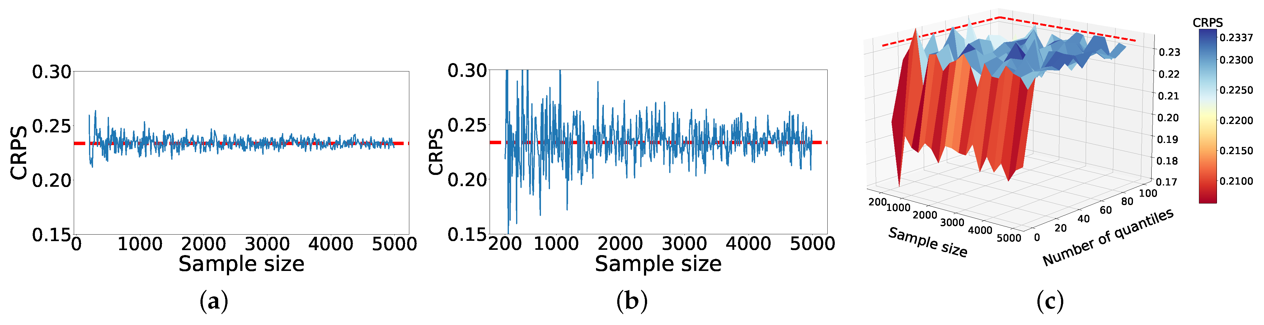
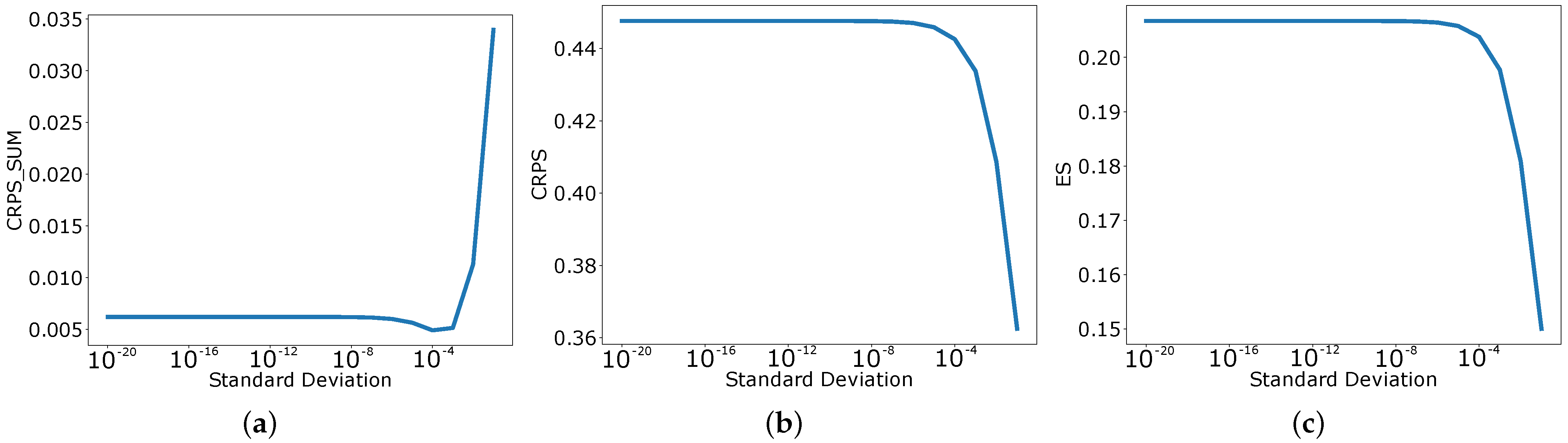
To investigate the significance of sample size on the accuracy of different approximation methods, we ran a simple experiment. In this experiment, we assumed that the probabilistic model follows a Gaussian distribution with $\sum =0$ and $\sigma =1$. Then, we approximated CRPS$(F,x)$ where $x=0$ with various sample sizes in range $[200,5000]$. Since we know the probabilistic model distribution, we can calculate the value of CRPS analytically, i.e., CRPS$(F,x)\approx 0.2337$.

From Figure 1a,b, we can perceive that the empirical CDF method and sample estimation method can converge to the close vicinity of the true value efficiently. However, the empirical CDF method has less variance in comparison to sample estimation. The method based on pinball loss depends on sample size and the number of quantiles. Figure 1c portrays how these two factors affect the approximation. We can see that with a number of quantiles greater than 20, the pinball loss method can produce a very good approximation using only a few samples (circa 500 samples).

3.2. Energy Score (ES)

Energy Score (ES) is a strictly proper scoring rule for multivariate time series. For an m-dimensional observation x in ${\mathbb{R}}^m$ and a predictive cumulative distribution function F, the energy score (ES) [28] is defined as

$$\mathrm{ES}(F,\mathbf{x})={\mathrm{E}}_F{\parallel \mathbf{X}-\mathbf{x}\parallel }^{\beta }-\frac{1}{2}{\mathrm{E}}_F{∥\mathbf{X}-{\mathbf{X}}^{\prime }∥}^{\beta },$$

(9)

where $∥.∥$ denotes Euclidean distance and $\beta \in (0,2)$. We can see here that CRPS is a special case of ES, where $\beta =1$ and $m=1$. While ES is a strictly proper scoring rule for all choices of $\beta$, the standard choice in application is normally $\beta =1$ [28].

ES provides a method for probabilistic forecast model assessment which works well on multivariate time series. Unfortunately, ES suffers from the curse of dimensionality [29] and its discrimination power decreases with increasing numbers of data dimensions. Still, the performance of ES in lower dimensionalities complies with the expected behavior of an honest and careful assessor. Hence, we can use its behavior in lower dimensionalities as the reference for comparison with newly suggested assessment methods.

3.3. CRPS-Sum

To address the limitation of ES in multidimensional data, Salinas et al. [18] introduced CRPS-Sum for evaluating a multivariate probabilistic forecasting model. CRPS-Sum is a proper scoring rule, and it is not strictly proper. CRPS-Sum extends CRPS to multivariate time series with a simple modification. It is defined as

$$\mathrm{CRPS-Sum}={\mathrm{E}}_t\left[\mathrm{CRPS}\left(F_{sum}^{-1},\sum _i{x}_t^i\right)\right],$$

(10)

where $F_{sum}^{-1}$ is calculated by summing samples across dimensions and then sorting to obtain quantiles. Equation (10) calculates CRPS based on the quantile-based method (Equation (7)). In a more general sense, one can calculate the CRPS-Sum by summing both samples and observations across the dimensions. This way, we would acquire a univariate vector of samples and observation. Then, we can apply any aforementioned approximating methods to calculate CRPS-Sum.

4. Investigating CRPS-Sum Properties

CRPS-Sum has been widely welcomed by the scientific community, and many researchers have used it to report the performance of their models [18,19,20,21]. However, the capabilities of CRPS-Sum have not been investigated thoroughly, unlike the vast studies dedicated to the properties of ES and CRPS [28,29,32]. To evaluate the discrimination ability of CRPS-Sum, we conducted several experiments on a toy dataset and outline the results in this section.

4.1. CRPS-Sum Sensitivity Study

In this study, we inspected the sensitiveness of CRPS-Sum concerning the changes in the covariance matrix. This study extends the sensitivity study that was previously conducted by [29,32] for various scoring rules, including CRPS and ES. For easier interpretation of the scoring-rule response to changes in a model or data, we defined relative changes in the scoring rule ${\Delta }_{\mathrm{rel}}$.

We ran our experiment N times, where ${\mathrm{CS}}_i$ denotes the obtained CRPS-Sum from the i-th experiment. We define

$$\begin{array}{c}\hfill \overline{\mathrm{CS}}=\frac{1}{N}\sum _{i=1}^N{\mathrm{CS}}_i,\end{array}$$

(11)

as the mean value of CRPS-Sum for the N experiments. Furthermore, let ${\mathrm{CS}}^{*}$ signify the CRPS-Sum for a model that is identical to the true data distribution. Now, the relative changes [29] in CRPS-Sum is defined as

$${\Delta }_{\mathrm{rel}}\left(\mathrm{CS}\right)=\frac{\overline{\mathrm{CS}}-{\overline{\mathrm{CS}}}^{*}}{{\overline{\mathrm{CS}}}^{*}}.$$

(12)

This metric frames the relative changes in the CRPS-Sum of a forecasting modeling across our experiments as the differences between the predicted and actual density of the stochastic process. The main idea is to determine the sensitivity of the scores with respect to some biased non-optimal forecast in a relative manner.

In this study, we have a true data distribution that follows a bivariate normal distribution with $\sum =\left(\begin{array}{c}0\\ 0\end{array}\right)$ and $\Sigma =\left(\begin{array}{cc}1& \rho \\ \rho & 1\end{array}\right)$ where $\rho \in [-1,-0.8,\dots ,0.8,1]$. Furthermore, we specified a forecasting model f that follows the same distribution; however, this time the off-diagonal element of the covariance matrix is $\varrho \in [-1,-0.9,-0.8,\dots ,0.8,0.9,1]$. In our study, we sampled $n=2^{14}$ windows of size $w=2^9$, as suggested in [32].

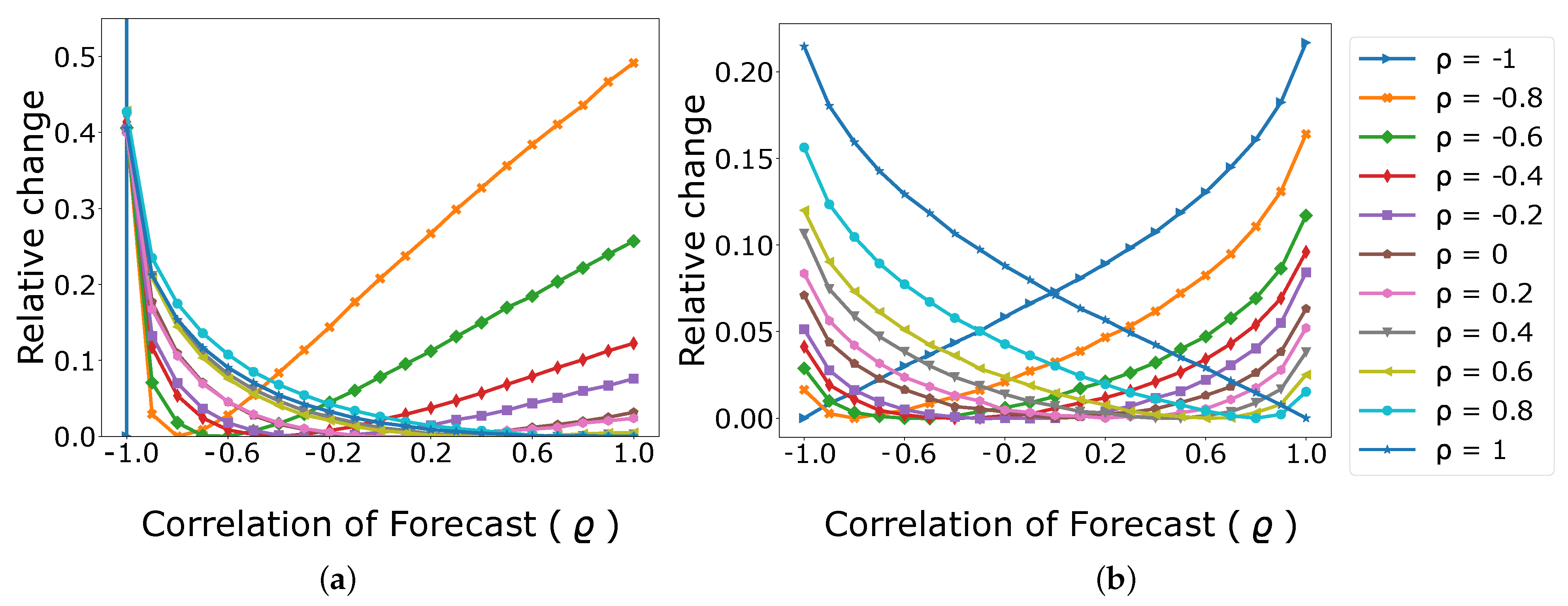
Figure 2 illustrates the relative change in CRPS-Sum and ES with respect to changes in correlation $\rho$ of the data-generating process as a function of the correlation coefficient $\varrho$ of the family of models we studied. We can observe that ES behavior is unbiased with regard to $\rho$ and its figure is symmetric. This is the expected behavior from a scoring rule in this scenario. In contrast, the response of CRPS-Sum to change in $\rho$ is not symmetric. It is more sensitive to the changes when the covariance $\rho$ of the data is negative, and it is almost indifferent to the changes when the covariance $\rho$ of the data is positive.

Hence, the sensitivity of CRPS-Sum to changes in covariance is dependent on the dependency structure of true data. In real-world scenarios, where we do not have access to the covariance matrix of the data-generative process, we cannot reliably interpret CRPS-Sum and compare various models based on CRPS-Sum.

4.2. The Effect of Summation on CRPS-Sum

To calculate CRPS-Sum, first, we summed the time-series over the dimensions [18]. Although this aggregation let us turn a multivariate time series into a univariate one, we lost important information concerning the performance of the model in each dimension. Furthermore, the values of dimensions that are negatively correlated negate each other and, consequently, those dimensions will not be presented in aggregated time series.

For instance, assume we have a multivariate time series x with two dimensions. Our data follow a bivariate Gaussian distribution with $\sum =\left(\begin{array}{c}0\\ 0\end{array}\right)$ and $\sum =\left(\begin{array}{cc}1& -1\\ -1& 1\end{array}\right)$. Hence, the following relation holds between dimensions:

$$x^0=-x^1.$$

(13)

By summing over dimensions, we have:

$$\begin{array}{cc}\hfill \sum _i{x}^i& =0.\hfill \end{array}$$

(14)

Clearly, after summation, we acquire a signal with constant zero, and all the information regarding the variability of the original time series is lost.

To acquire information regarding the performance of the model on each dimension, we can calculated CRPS first. Once the CRPS was validated, we could calculate the CRPS-Sum to check how well the model learned the relationship between the dimensions, and even, at this point, we should not forget the flaws of CRPS-Sum that we witnessed, e.g., sensitivity toward data covariance and loss of information during summation. Unfortunately, the importance of CRPS is ignored in most of the recent papers in the probabilistic forecast domain. In these papers, the CRPS is either not reported at all [20,21], or the argument about the performance of the model is made solely based on CRPS-Sum [18,19]. Considering the flaws of CRPS-Sum, this trend can put the assessment results of these recent models in jeopardy.

5. Closer Look into CRPS-Sum in Practice

In the previous section, we discussed the properties of CRPS-Sum and indicated its shortcomings in hypothetical scenarios using toy data settings. In this section, we aim to investigate CRPS-Sum capabilities with real datasets. To do so, we conducted experiments by constructing simple models that are based on random noise and investigate their performance using CRPS-Sum. In our first experiment, we employed the exchange-rate dataset [35]. The exchange-rate dataset is a multivariate time series dataset which contains the daily exchange rate of eight countries, namely, Australia, British, Canada, Switzerland, China, Japan, New Zealand, and Singapore, which was collected between 1990 and 2016. This dataset has few dimensions, which lets us use ES alongside CRPS and CRPS-Sum. Additionally, it is easier to perform qualitative assessment on lower dimensionalities. We used the dataset in the same setting that is proposed in [18].

We also utilized the low-rank Gaussian copula processes method (GP-copula) from [18]. GP-copula combines an RNN-based time-series model with a Gaussian copula process output model for probabilistic forecasting. Furthermore, the model employs a low-rank covariance structure to reduce the computational complexity and handle non-Gaussian marginal distributions. We selected this model since the model performance has been reported in CRPS-Sum.

Our first model is a dummy univariate model which follows a Gaussian distribution. The mean of the Gaussian distribution is $\sum ={\sum }_{last}$ where ${\sum }_{last}$ is the mean of the last values in the input vector over the dimensions, i.e.,

$${\sum }_{last}=\frac{1}{D}\sum _{i=1}^D{x}_T^i.$$

(15)

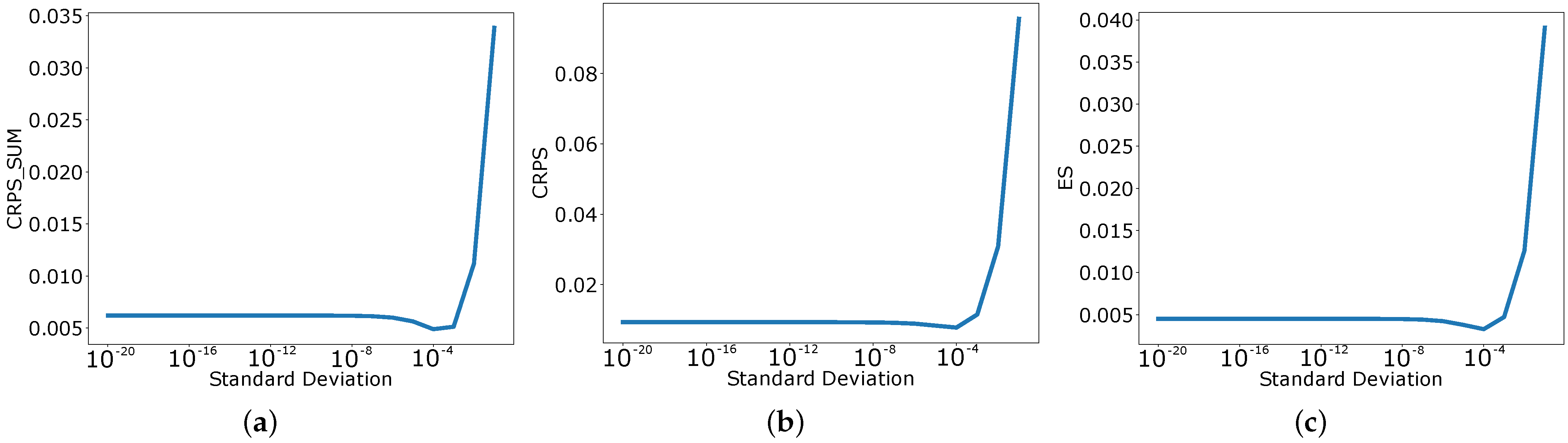
We used $\sigma ={10}^{-4}$ as the standard deviation of the dummy univariate model in our experiments; however, the results are not dependent on the $\sigma$ value (more discussion on $\sigma$ values can be found in Appendix B). We used this model to generate the forecast for every dimension.

For the second model, we employed a multivariate Gaussian distribution to build a dummy multivariate forecaster. The mean of the i-th dimension of the multivariate Gaussian distribution is the value of the last time step in the input window, i.e., ${\sum }_i=x_T^i$. The covariance matrix is zero everywhere except on its main diagonal, which is filled with ${10}^{-4}$. In other words, we extended the last observation of the input window as the prediction and apply a small perturbation from a Gaussian distribution.

Table 1. This table illustrates the results from dummy models on the exchange-rate dataset and compares their performance with GP-copula based on CRPS-Sum, CRPS, and ES. It shows that CRPS-Sum dummy models have better performance in comparison to GP-copula.

	GP-copula	Dummy Univariate	Dummy Multivariate
CRPS-Sum	0.0070	0.0049	0.0048
CRPS	0.0092	0.4425	0.0077
ES	0.0043	0.2037	0.0032

presents the CRPS-Sum, CRPS, and ES of the two dummy models and the result of the GP-copula model from [18] on the exchange-rate dataset. Note that all values in this paper were calculated using the sampling method. We calculated these metrics based on the quantile method as well, which yielded almost similar results. While the CRPS-Sum suggests that the dummy univariate model is much better than GP-copula, the CRPS and ES indicate that the performance of the dummy univariate model is worse than GP-copula. The results reported by CRPS and ES are aligned with our expectations; however, the CRPS-Sum reports a misleading assessment.

On the other hand, the quantitative results for the dummy multivariate model are quite surprising. All three assessment methods denote that the dummy multivariate has a superior performance in comparison to GP-copula. To provide further explanation for this unexpected result, we analyzed the performance of these models qualitatively.

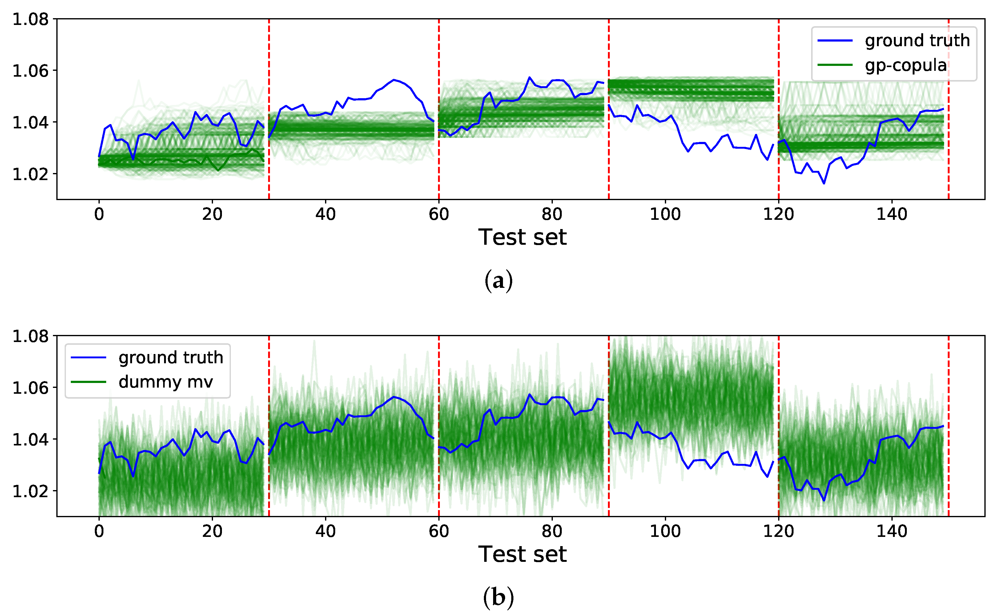
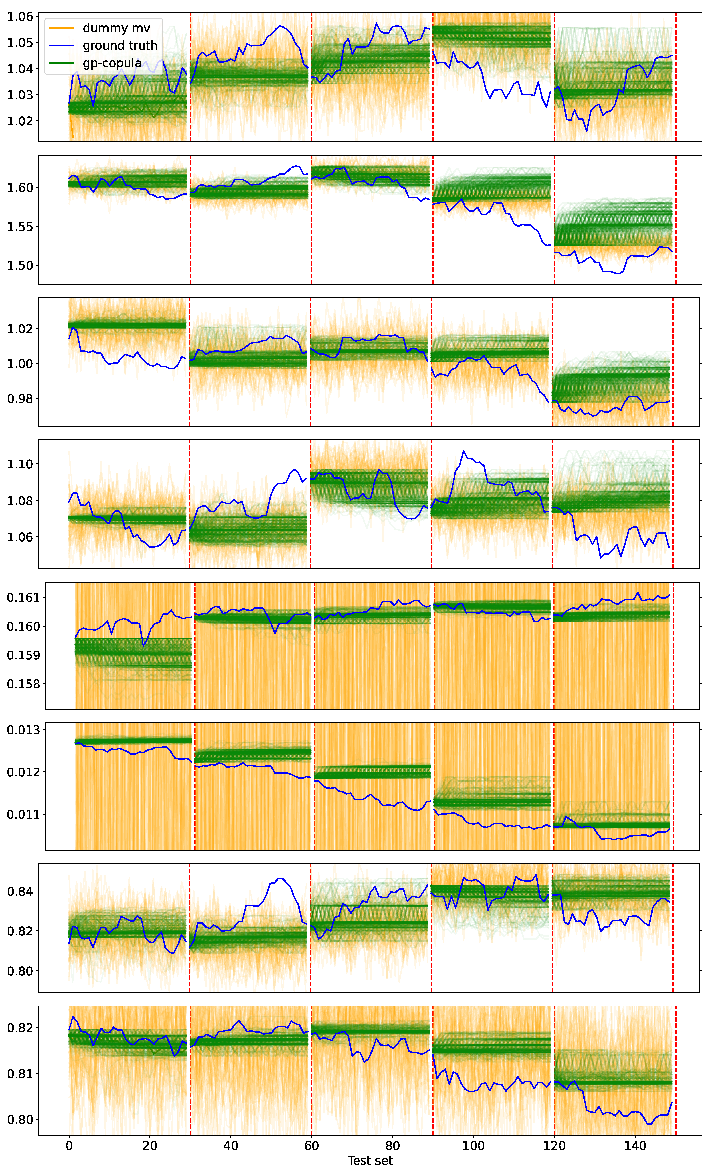
Figure 3a depicts the forecasts from GP-copula for the first dimension of the exchange-rate dataset (the rest of the dimensions are visualized in Appendix A) and Figure 3b presents samples from the dummy multivariate model.

This experiment shows us that the border between a dummy model and a genuine model can become very blurry if we rely solely on CRPS-Sum. Furthermore, we learn that CRPS and visualization can help us to acquire a better understanding of model performance.

In the second experiment, we performed a similar experiment on the taxi dataset [36]. The taxi dataset contains the spatio-temporal traffic time-series of New York taxi rides taken at 1214 locations every 30 min in the months of January 2015 (training set) and January 2016 (test set). This dataset consists of 1214 dimensions.

Table 2. This table illustrates the results from dummy models on the taxi dataset and compares their performance with GP-copula based on CRPS-Sum, CRPS, and ES. In contrast to the exchange-rate dataset, it is not feasible to cross-check these quantities in higher dimensionalities.

	GP-copula	Dummy Univariate	Dummy Multivariate
CRPS-Sum	0.1703	0.4685	0.4705
CRPS	0.3336	0.6778	0.7543
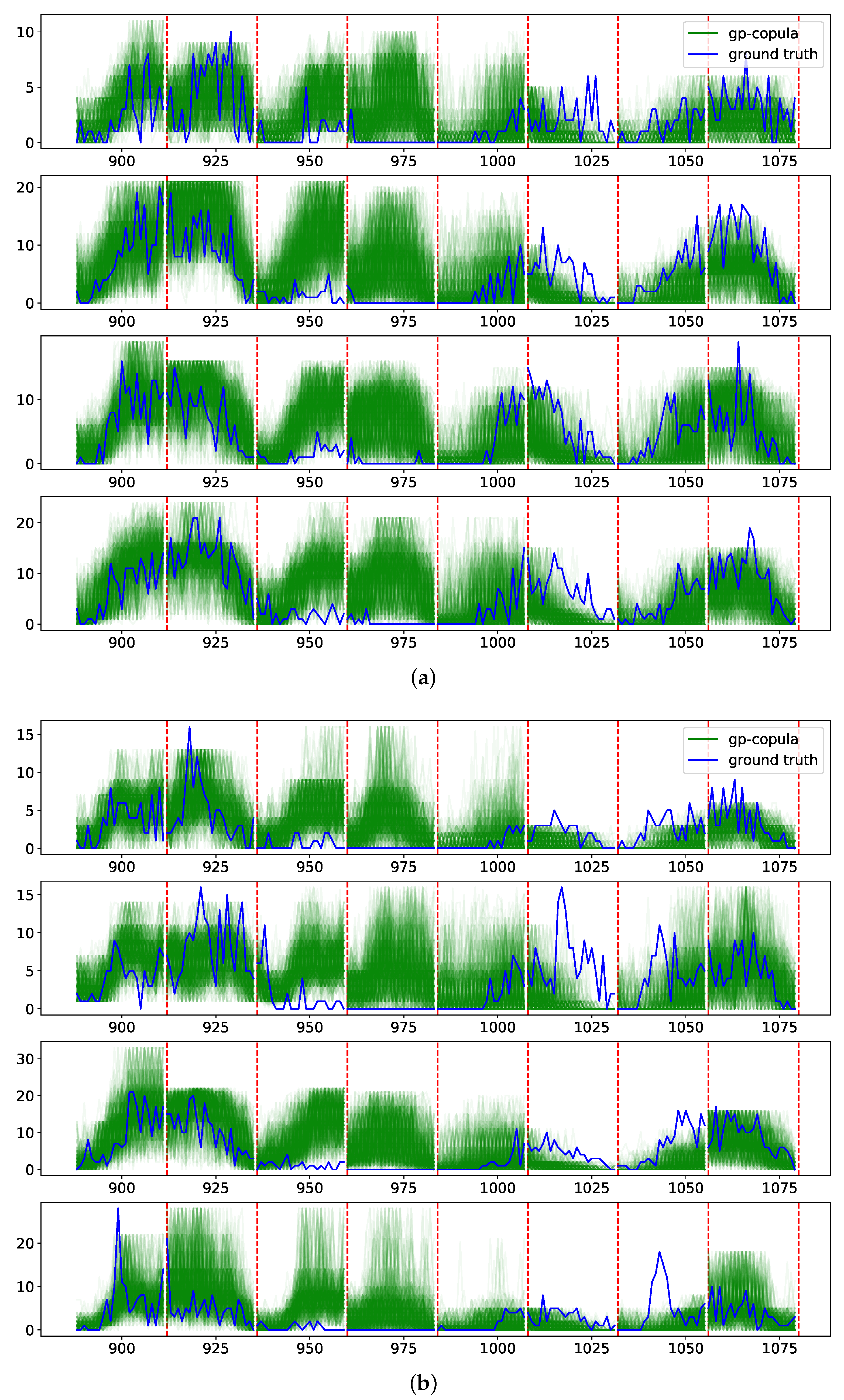
ES	0.0138	0.0284	0.0318

presents results for the experiment on the taxi dataset. In contrast to the previous experiment on the exchange-rate dataset, we cannot examine the discrimination ability of CRPS-Sum by comparing it to other metrics in higher dimensionalities. As mentioned in Section 3.2, the ES is not a reliable indicator of model performance in higher dimensionalities. CRPS cannot reflect the dependency structure learned by the model. Furthermore, we cannot crosscheck the CRPS-Sum discrimination ability with the qualitative performance of the model, since it is not possible to investigate the model’s performance intuitively due to the size of data and the unintuitive nature of time-series data. For instance, Figure 4a,b illustrates the performance of GP-copula on the dimensions where the model has the best and the worst performance based on CRPS. By comparing these two figures, we can perceive clearly that the qualitative analysis of model performance is not feasible and straightforward. This experiment emphasizes again the importance of a strictly proper scoring rule for probabilistic multivariate time-series forecasting, which is sound in its definition and analyzed carefully with real-world datasets with low dimensionalities.

6. Conclusions

In this paper, we reviewed various existing methods for the assessment of probabilistic forecast models and discussed their advantages and disadvantages. While CRPS is only applicable to univariate models and ES suffers from the curse of dimensionality, CRPS-Sum was introduced to help us with assessing multivariate probabilistic forecast models. Unlike CRPS and ES, the properties of CRPS-Sum have not been studied in the past. Our sensitivity study illustrates that the CRPS-Sum behavior is not symmetric concerning the covariance of data distribution. CRPS-Sum is more sensitive to changes in the covariance of the model when the covariance of the data is negative. This is an undesirable behavior and makes result interpretation difficult.

Furthermore, CRPS-Sum cannot reflect the performance of a model on each dimension due to the loss of information caused by summation during its calculation. We demonstrated this problem with simple examples and experiments on the exchange-rate dataset, where a dummy model based on random noise achieved better CRPS-Sum than the state-of-the-art model. Additionally, with the experiment on the taxi dataset, we portrayed that the study of the CRPS-Sum discrimination ability in higher dimensionalities is not feasible.

To conclude, CRPS-Sum cannot provide an unbiased and accurate assessment for multivariate probabilistic forecasters. Thus, we suggest avoiding CRPS-Sum if possible. For data with low dimensionality, we can use ES. In higher dimensions, the assessment of the probabilistic forecast model is still an open problem. In the current state, it is difficult to rely solely on any existing metric and manual qualitative analysis should be used to evaluate the performance as well.

7. Future Works

Considering the shortcomings of CRPS-Sum, there is an urgent need for an assessment metric for multivariate probabilistic forecast models. A desirable metric would be a strictly proper scoring rule that summarizes the model performance in a single value using a reasonable number of samples. Furthermore, it should be capable of reflecting the precision of the model in learning the probability distribution of each dimension, as well as model accuracy in capturing cross-dimension dependencies. Additionally, it is desirable to investigate the discrimination ability of such metrics using various probabilistic forecasting methods on multiple real-world datasets.