Improving PM2.5 Concentration Forecast with the Identification of Temperature Inversion

Abstract

The rapid development of industrialization and urbanization has had a substantial impact on the increasing air pollution in many populated cities around the globe. Intensive research has shown that ambient aerosols, especially the fine particulate matter PM_2.5, are highly correlated with human respiratory diseases. It is critical to analyze, forecast, and mitigate PM_2.5 concentrations. One of the typical meteorological phenomena seducing PM_2.5 concentrations to accumulate is temperature inversion which forms a warm-air cap to blockade the surface pollutants from dissipating. This paper analyzes the meteorological patterns which coincide with temperature inversion and proposes two machine learning classifiers for temperature inversion classification. A separate multivariate regression model is trained for the class with or without manifesting temperature inversion phenomena, in order to improve PM_2.5 forecasting performance. We chose Puli township as the studied site, which is a basin city easily trapping PM_2.5 concentrations. The experimental results with the dataset spanning from 1 January 2016 to 31 December 2019 show that the proposed temperature inversion classifiers exhibit satisfactory performance in F1-Score, and the regression models trained from the classified datasets can significantly improve the PM_2.5 concentration forecast as compared to the model using a single dataset without considering the temperature inversion factor.

1. Introduction

The growth of economic and industrial development inevitably threatens the preservation of the natural environment. One of the sustainable development goals is to promote green trade, which produces low carbon levels during product manufacturing, transportation, use, and end-use disposal. Some of the production emissions are toxic, especially for the particulate matter of diameter ≤ 2.5 μm (PM_2.5), and they can significantly spoil human health. Many researches have shown that PM_2.5 concentrations are greatly related to respiratory diseases [1] and cancer development [2]. It is reported by World Health Organization (WHO) that nearly 3 million people were killed due to ambient PM_2.5 in 2012 [3].

The apportionment of PM_2.5 covers a wide range of chemicals such as sulfate, nitrate, ammonium, carbonaceous compounds, crustal elements, organic compounds, and free radicals [4]. These chemical compositions come from three main sources [5]: natural, anthropogenic, and secondary transformation. The natural source comes from environmental soil dust, crustal elements, volcanic eruptions, sea salt, biomass, etc. The anthropogenic source is emitted from the economic activities ranging from vehicle exhaust, burning, coal and gasoline combustion, to petrochemical production and steel refinery. The secondary transformation source is contributed by photochemical reactions of precursors such as SO₂ and NO_x. The air pollution incurred by these sources may influence different-sized over various durations. The size of the pollution area could be small such as incense burned during temple worship. Vehicle traffic usually causes a line pollution along the roads. For pollution resulting from volcanic eruptions or large petrochemical complexes, the area of pollution coverage can be as large as a city.

PM_2.5 pollution, once emitted from various sources, will drift in the air and transport to downstream zones. Some particular geographic terrains such as valleys, basins, and hillsides could easily trap the PM_2.5 flow to collectively concentrate at local regions. Usually, the concentration lasts for several hours and scatters away with wind flows. However, it may last for several days if the weather condition prevents the concentration from scattering. One such notorious weather condition is the temperature inversion which forms a warm-air cap above the cooler ground surface, trapping the PM_2.5 concentrations under the warm-air cap.

Temperature inversion is a commonly appearing scenario in Taiwan and frequently causes high PM_2.5 concentrations at particular places. This paper chooses Puli township as the study site because it is a basin surrounded by mountains and often sees temperature inversion. We observe that there is high association between the occurrence of high PM_2.5 incurred by temperature inversion and some weather patterns. One such pattern is that there is no precipitation and the wind is relatively calm. If the temperature inversion phenomenon can be recognized by analyzing the weather patterns, we speculate that the estimation of PM_2.5 concentration based on regression of weather variables would be more accurate.

The contributions of this paper include the following. (1) Many researches have shown that temperature inversion is one of the leading causes for observing high PM_2.5 concentrations. Puli is a basin township which easily seduces temperature inversion. To the best of our knowledge, there is no existing research which analyzes the meteorological scenarios of temperature inversion for improving the PM_2.5 prediction performance. This paper presents the first proposal in this research direction. (2) To construct a more effective model for PM_2.5 concentration forecasting, two machine-learning-based classifiers, namely, the CART (classification and regression trees) and CNN (convolutional neural networks), are developed to distinguish the test days into two classes. One class includes the days with temperature inversion, the other class includes the rest. The classification performances of the two classifiers are compared in terms of various metrics. (3) The meteorological features of the two training classes are contrasting and they have different relationships with the PM_2.5 concentrations. A separate regression model for PM_2.5 forecasting is trained for each group to enhance the overall prediction performance. (4) Our experimental results with the Puli PM_2.5 and meteorology datasets during the period from 2016 to 2019 show that the models considering the temperature inversion factor reduce the forecast errors by 4–9% and 2–7% in terms of RMSE and MAE, as compared to the original model.

The remainder of this paper is organized as follows. Section 2 reviews the relevant researches on analyses of PM_2.5 concentrations in Taiwan, temperature inversion phenomenon, and existing PM_2.5 estimation approaches. Section 3 elucidates the proposed method for PM_2.5 forecast. Section 4 presents the experimental results and comparative performances. Finally, Section 5 concludes this work.

2. Literature Review

2.1. Analysis of PM_2.5 Concentration in Taiwan

The west coast of central and southern Taiwan, which accommodates petrochemical complexes, coal combustion power plants, industrial parks, and national highways, is notorious as one of the heaviest-polluting regions in Taiwan [6]. Moreover, the PM_2.5/PM₁₀ ratio for central and southern Taiwan is around 61–67%, which is higher than the 54–59% measured for northern Taiwan [7]. These studies show that the air pollution in central and southern Taiwan is not only higher than that in northern Taiwan, but its apportionment is also more harmful to human health. Several studies have been conducted in these regions to explore the pollution apportionment and transportation routes. The back trajectory model was applied in [8] and it was found that winter aerosols concentrate at Changhua county because of the northwestern wind passing over Mongolia, northern China, and central-western Taiwan. Meanwhile, the southwestern wind in spring and summer blows the soil and crustal elements in the air from the river banks and carries the emissions from coal and oil combustions at the petrochemical complex and the power plants. A case study of 22 polycyclic aromatic hydrocarbons (PAHs) was conducted in the same place [2]. The receptor-based apportionment model is applied to analyze the PAH compounds. The lifetime excess cancer risk (ECR) from inhalation exposure to PAHs is 4.7 × 10⁻⁵, which is nearly fifty times higher than the guideline limit (10⁻⁶) released by United States Environmental Protection Agency (USA EPA). Hsu and Cheng [6] studied the meteorological influence on PM_2.5 concentrations in Yunlin County which is near to two large-scale coal-fired power plants and one petrochemical complex. It is shown that the weather pattern with a continental anticyclone or a stagnant local circulation results in high PM_2.5 concentrations from industrial production. Kaohsiung is another southern Taiwanese city which has high pollution concentrations due to industrialization. Kuo et al. [9] studied the factors most influencing PM_2.5 intensities in Kaohsiung and found that the most abundant PM_2.5 chemical components were ${\mathrm{SO}}_4^{2-}$, ${\mathrm{NO}}_3^{-}$, elemental and organic carbon. ${\mathrm{SO}}_4^{2-}$ constitutes 29.8% of the PM_2.5 mass and it is formed by the oxidation of SO₂ emitted from diesel vehicles and coal/oil combustion which are strongly related to oil and steel industries in Kaohsiung. A population-based study [10] conducted by Chang Gung Memorial Hospital (the largest medical service system in Taiwan) in 2012 showed that the number of emergency room visits for respiratory disease are highly associated with the increase in ambient PM_2.5 concentrations. This phenomenon is more significant for southern Taiwanese districts.

Aside from the industrial production and traffic emissions, some particular anthropogenic activities occasionally trigger pollution events. On every 9 January of the lunar calendar, Taoists burn incense and joss papers at homes and temples to celebrate the birthday of the First God. A case study [11] has shown that there is a rapid increase of PM_2.5 concentrations in almost all residential regions of Taiwan during the religion ritual. In Chinese custom, families gather outdoors to attend moon-watching activities at the Mid-Autumn Festival (MAF) Day (15 August of the lunar calendar). In Taiwan, the moon-watching activities are a barbecue festival, and many people gather at households or in the streets. Tsai et al. [12] studied the relationship between the MAF phenomenon and the PM_2.5 variations. The result shows that the PM_2.5 mass concentration is the highest during the MAF, followed by the period leading up to the MAF, and it is the lowest after the MAF.

In addition to locally produced pollutions, long-range transported pollutions from other countries significantly affect Taiwan’s air quality during different seasons and weather conditions. For instance, every autumn pollutants are carried into Taiwan by the northeast monsoon [13], and in spring the air quality of Taiwan is usually spoiled by north Asian dust storms [14] and the ambient particles transported from northern China [15].

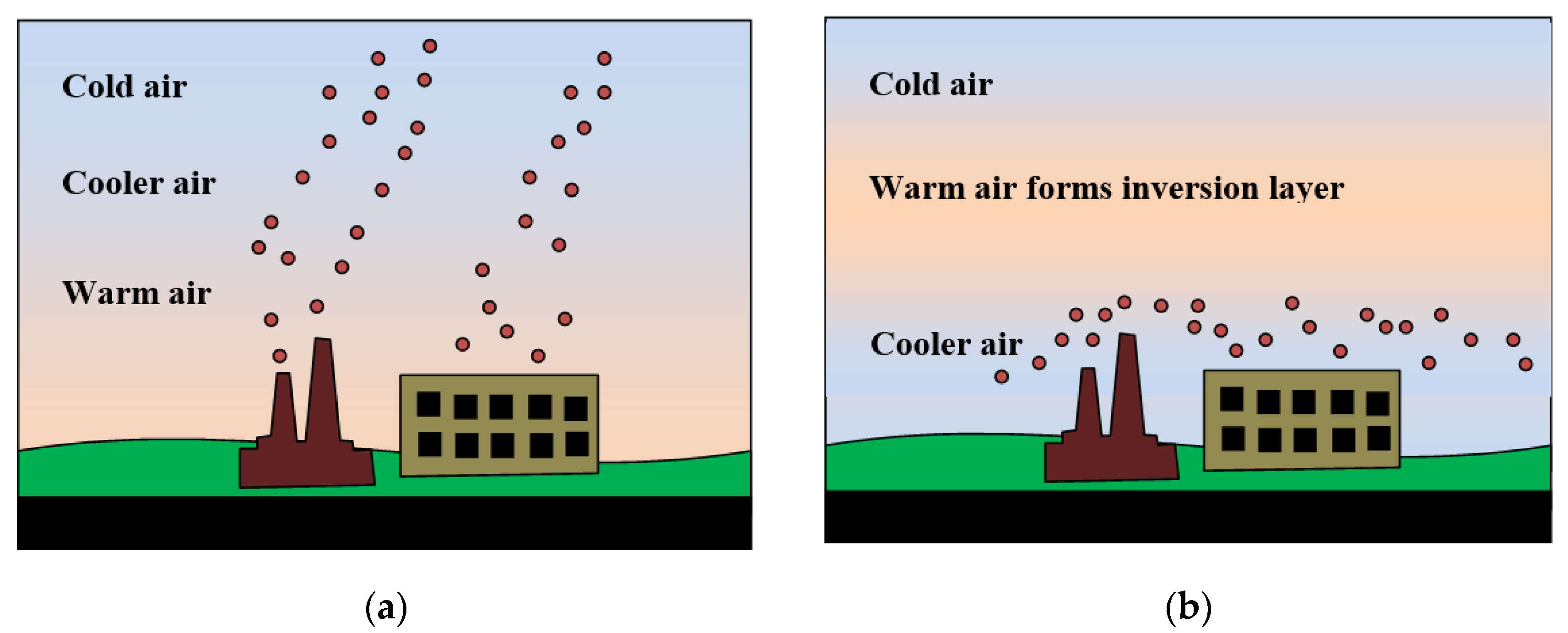
2.2. Temperature Inversion

Air pollution is more serious under particular atmospheric stagnation conditions. Normally, the temperature in the troposphere (from 0 to 11,000 m elevation) decreases by 0.65 degrees Celsius for every 100 m of elevation. The temperature variation phenomenon promotes the convection of aerosols (see Figure 1a). However, at occasional weather conditions such as the radiation cooling at night, the cold air plunges down through the warm air and the warm air forms a cap above the ground-level cold air, causing the temperature layer to be inversed. Such temperature inversion will trap the convection of the surface air limited below the warm-air cap and exacerbate the air pollution as shown in Figure 1b [16,17]. It was indicated in [18] that the PM_2.5 concentration is raised up by 54% due to the temperature inversion at the three observation sites investigated in their study. Tran and Mölders [19] investigated the pollution days observed in Fairbanks, Alaska, and they found that all of the 128 winter pollution days during the period between 2004 and 2009 are related to phenomenon of the temperature inversion.

Puli in Taiwan is a basin township surround by mountains 1000 to 2000 m tall, easily encouraging temperature inversion at nights. Air pollution is therefore hard to dissipate if the wind is calm. This motivates us to explore the relationship between meteorological variables (air pressure, temperature, relative humidity, and wind speed) of temperature inversion and the PM_2.5 concentrations, in order to enhance the prediction accuracy by discriminating between the days with and without temperature inversion. We hypothesize that such a prevailing predictor for PM_2.5 concentrations can be trained by partitioning the training data into the two salient classes.

2.3. PM_2.5 Forecasting

The existing PM_2.5 forecasting approaches fall into three prevailing categories. (1) Regression or autoregression methods: The regression methods require explanatory variables in addition to the PM_2.5 series itself, while the autoregression methods need only the PM_2.5 series. Regression methods can be effective if the selected explanatory variables are informative and sufficient to describe the PM_2.5 concentrations. The widely used explanatory variables include wind speed and direction, precipitation, temperature, relative humidity, atmospheric pressure, land use, traffic amount, road types, satellite images, to name a few. The effectiveness of each explanatory variable depends on the climate ecology and anthropogenic activities in the studied location. Both linear [20,21,22] and nonlinear [23,24,25] regression models have been employed in the literature. Autoregression methods focus on discovering the temporal trends contained in the PM_2.5 time series. Autoregressive integrated moving average model (ARIMA) was adopted in [26] to explore the short-term time series and estimate the mean daily PM_2.5 concentration. Generalized autregressive conditional heteroscedasticity (GARCH) model was used in [27] to capture linear and nonlinear panel information for PM_2.5 concentrations forecasting. (2) Machine learning methods: Among others, support vector machine (SVM) and artificial neural networks (ANN) are the most popular ones. Mogollón-Sotelo et al. [28] constructed an SVM to forecast PM_2.5 concentrations in Bogotá which is a tropical city with complex terrains. The SVM model is trained to represent the behavior of days with high PM_2.5 concentrations and those with fast changes in PM_2.5 tendency. An SVM was developed in [29] for PM_2.5 class prediction. Three most relevant meteorological variables are extracted by measuring the cosine similarity among records in the same PM_2.5 class. With the identified meteorological variables, the SVM is trained to make the classification. The training parameters of the SVM are optimized by the particle swarm optimization (PSO) algorithm to improve the classification accuracy. A specific type of ANN named multiple layer perceptron (MLP) is adopted in [30] to learn the relationship between PM_2.5 concentration and a set of meteorological factors with satellite-derived AOD data. An ensemble model was established in [31] to combine PM_2.5 estimates from three machine-learning methods, namely, neural network, random forest, and gradient boosting. A deep-learning long short-term memory (LSTM) model was proposed in [32] for predicting daily PM_2.5 concentration in China. The spatiotemporal information of surrounding monitoring stations is used to adjust the prediction model. Another deep learning network consisting of a CNN and an LSTM was deployed in [33]. The CNN is designed to extract meteorological features from 14 sites in Shanghai and the LSTM is used to model time dependence of pollutants. (3) Hybrid methods. An increasing number of recent works developed hybrid approaches which boost the performance by complementing the strengths and weaknesses of individual models. In particular, regression has been hybridized with ANN [34] and SVM [27]. It is worth noting that most hybrid methods combine complementing models to build a stronger predictor. To the best of our knowledge, none has intended to combine contrasting machine-learning models in various phases such as meteorological pattern classification and PM_2.5 concentration prediction as we have in our paper.

Different periods of training time span have been considered in the literature, ranging from a couple of days covering a pollution event, a monsoon season, an entire year, to a longer-term multiyear dataset [11,12,25,27]. Training on different periods of time span may obtain distinct relationship between PM_2.5 concentrations and the investigated variables. For instance, the relationship between temperature and PM_2.5 concentrations varies with the investigated season. The plots for the data collected in Puli EPA supersite for different seasons in 2016 manifest diverse temperature vs. PM_2.5 patterns (see Figure 2a). The PM_2.5 concentrations generally grow linearly with the temperature in summer (see Figure 2b), while the relationship converts to a complex nonlinear form in autumn as shown in Figure 2c. If we use all data to express the relationship, the descriptive power of the investigated variables will decrease. Analogously, training on different datasets having distinct properties such as temperature inversion or stationary front, the resulted learning model will perform differently on unseen data. Few studies have noticed this problem. In this paper, two training datasets are used to produce more descriptive-power relationship functions for the designated datasets. One training class includes the data for those days in a year which belong to the detected temperature inversion class, the other contains data in the seven days immediately preceding the test day. In other words, we consider temperature inversion as a specific type of meteorological phenomenon and an effective PM_2.5 forecasting model can be trained on such instances. While for the days without temperature inversion, the relationship between PM_2.5 concentration and meteorological variables is more influenced by the short-term data in the preceding week.

3. Proposed Methods

3.1. Materials

As seen in Figure 3a, Puli is located in central Taiwan and is to the east of two potential pollution sources, the largest coal combustion power plant in Taichung city and a petrochemistry complex in Yunlin county. The landscape of Puli is a basin sitting at 100 m above sea level and surrounded by mountains. The mountains climb up from the west to the east of Puli with heights from 1000 to 2000 m, as shown in Figure 3b. As there is a river going across Puli, the main inlet for the external pollutions flowing into the basin is through the west river valley (indicated by red arrow). The highway 6, which is the major transportation route carrying goods from the west into Puli, was built along the river. The busy highway traffic also produces PM_2.5 concentrations. It is often observed that once the pollutants arise, they last longer in the Puli basin area than in the western metropolitan areas. This situation gets even worse in those days with temperature inversion. As the Taiwan Environmental Protection Administration (Taiwan EPA) deployed only one PM_2.5 monitoring supersite in Puli township (see the red dot in Figure 3b), we thus collected the PM_2.5 and the meteorological hourly data measured at the supersite (https://www.epa.gov.tw/ accessed on 10 December 2021). The time span of the collected data is between 1 January 2016 and 31 December 2019. The Taiwan EPA supersite applies the beta attenuation monitoring (BAM) technique for PM_2.5 measurement (https://airtw.epa.gov.tw/cht/EnvMonitoring/Central/Tools.aspx accessed on 10 December 2021). The BAM employs the energy absorption of beta radiation by suspended particles extracted from the air flow. The attenuation caused by suspended particles is exponentially dependent on the particle mass in the sample. We obtained the Puli meteorological dataset from the Taiwan Central Weather Bureau (http://e-service.cwb.gov.tw/HistoryDataQuery/ accessed on 10 December 2021) which tallies atmospheric pressure, temperature, relative humidity, wind speed and direction, and precipitation.

3.2. Feature Engineering

To select effective features for classifying the days into two classes, i.e., the days with and without temperature inversion, we consulted meteorologists to learn about commonly seen meteorological phenomena when temperature inversions arise. The prevailing phenomena are as follows. We usually see relatively high temperature around noon and relatively low temperature at night. The difference between the temperature at noon and at night is large as compared to other days in the same season. The correlation between the phenomena and the temperature inversion is more significant when the relative humidity is high and the wind is calm at night and there is no precipitation. However, the relative highs and lows for the meteorological measures vary from month to month. We thus applied k-means algorithm in Scikit-learn to automatically label the meteorological data into three classes according to individual monthly value ranges. For each of the meteorological measures (temperature, relative humidity, and wind speed) and PM_2.5 observations, we collected the hourly data within the same month and the k-means algorithm was used to label the hourly data for each measure into three classes: high (colored in red), middle (uncolored), and low (colored in green). However, the meteorological patterns depicted by meteorologists are weak. For example, the time period for measuring the noon temperature could be flexible. We may see relatively high temperature span through 11:00 a.m. to 2:00 p.m., or from 12:00 a.m. to 3:00 p.m. Both phenomena can be considered as relatively high noon temperature. The same situation applies to other meteorological patterns. In order to obtain ground-truth values of temperature inversion, we manually labeled each day as being with and without temperature inversion according to these weak patterns.

Figure 4 shows the data labeling for two plausible examples of temperature inversion phenomena. The left example is from 2016, the right one 2017. Both examples show that the temperature around noon was relatively high and started to cool down in the evening, and reached its monthly low range in the midnight. An opposite phenomena was observed for relative humidity, which showed a monthly low around noon and monthly high at night. The PM_2.5 collectively concentrated in the afternoon due to temperature inversion and the conditions of calm wind at night and no precipitation barricade the PM_2.5 concentrations to disperse. The PM_2.5 value reached its monthly highs before evening and usually stayed in this high class for more than eight straight hours. Conspicuously, the previously-noted phenomena about temperature, relative humidity, wind speed, and precipitation are salient features for classifying temperature inversion.

We further divided the days in 2016 and 2017 into two groups, the days with and without the noted meteorological phenomena, respectively. For each group, the mean hourly PM_2.5 concentration was evaluated. It is seen in Figure 5 that, for both years, the mean hourly PM_2.5 value with the noted phenomena was higher than that without the meteorological phenomena. The difference between the mean values of the two groups is more significant after evening and before dawn. This reveals that the two groups had very different conditions for raising PM_2.5 concentrations. We believe that if the two groups of days were separately analyzed, the prediction of PM_2.5 concentrations would be more accurate.

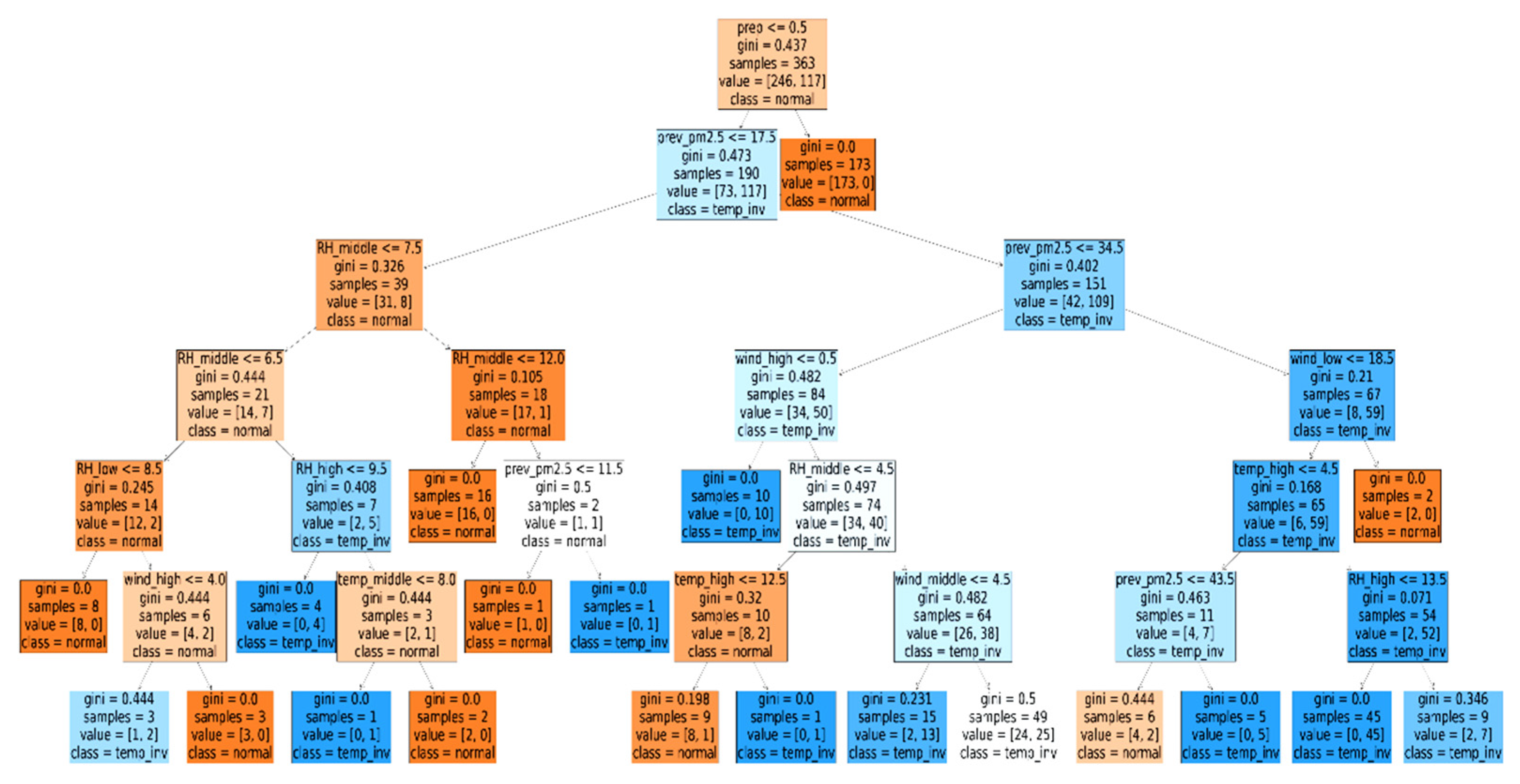
3.3. Temperature Inversion Classification

With the preliminary results of feature engineering, we selected the following features for designing the temperature inversion classification models: three categorical features (the labeling of hourly temperature, relative humidity, and wind speed, as high, middle, or low determined by k-means) and two numerical features (precipitation and PM_2.5 concentrations in the immediate previous day). Two classification models, CART and CNN, were chosen for comparative performance analyses.

CART [35] is an advanced decision tree algorithm. It can be applied to accomplish classification (with categorical target value) or regression (with continuous target value) learning tasks. CART is widely used because it is provided in the Scikit-learn library. The classification by CART proceeds as follows. A binary tree is grown to a specified maximum depth. At each level of depth, the feature which minimizes the Gini impurity is chosen to branch the inner node with an appropriate threshold into dichotomies. The Gini impurity is an estimate of the probability that a randomly chosen sample is misclassified. After the classification tree is fully grown, a pruning step with cross-validation is applied to reduce the tree complexity. Because the CART implementation provided by Scikit-learn currently does not support categorical variables, we converted our categorical features (temperature, relative humidity, and wind speed) to numerical ones by redefining them as the number of hours that each individual feature is labeled as each of the range classes (high, middle, and low). The previous day 24 h PM_2.5 concentrations were replaced by their mean value to reduce the number of similar features. Figure 6 shows the learned decision tree from the collected data in 2016 where three days had missing values and were removed and the data of the remaining 363 days were used as the training data. It is seen that the most salient rule for labeling the days as temperature inversion is as follows.

No precipitation, the previous day mean hourly PM_2.5 concentration is above 34, the number of low-wind-speed hours is less than 19, the number of high-temperature hours is greater than 4, and the number of high relative humidity hours is less than 14.

The second most significant rule is as follows.

No precipitation, the previous day mean hourly PM_2.5 concentration is between 18 and 34, and there is no high wind speed hours.

The CNN [36] has emerged as one of the main research streams in deep learning. A CNN adds several convolution layers in front of traditional neural networks such as the fully-connected multilayer perceptron. The convolution layer applies local convolution operations with different kernels/filters such that the local features contained in the original input image can be automatically extracted. The salient responses of these local features are retained by pooling operations. By concatenating several convolution layers, the features of various details and resolutions are learned. These features are fed forward to the traditional fully-connected networks to learn the weights and bias for the classification. Due to the increasing computing capability of processors such as GPUs, large CNN architectures which are able to learn classification for millions of images have been proposed. Ever since AlexNet [37] won the first prize of ILSVRC 2012, the development of CNN-based applications has been overwhelming. AlexNet improves the error rate by 10 percent as compared to the champion in ILSVRC 2011. AlexNet consists of five convolution layers followed by a two-layer fully-connected neural network. More recently, sophisticated CNNs such as GoogLeNet [38], ResNet [39], and SENet [40], have prevailed the ILSVRC competitions.

The design of our CNN architecture is as follows. The input layer receives data instances of 5 × 24 images which is composed of five selected features collected in straight 24 h. The five features are the temperature, relative humidity, wind speed, precipitation, and the previous day PM_2.5 concentrations. To accommodate monthly relative range, the features are encoded into numerical codes as 1 (low range), 2 (middle range), and 3 (high range) determined by k-means. Following the input layer, two repetitions of convolution layer and pooling layer are deployed. In the convolution layer, six 3 × 3 convolution kernels are applied to generate six feature maps with the ReLU activation function. Each feature map then goes through the max-pooling layer to extract the salient features. The same convolution-pooling architecture is constructed again to extract more generalized feature maps. Next, the feature maps are flattened to form a one-dimensional vector which is fed into the fully-connected network to produce the final output classification.

We trained the constructed CNN with the entire 2016 data whose 363 meteorological records were randomly assigned into training set and validation set respecting the size ratio of 8:2. Figure 7 shows the learning curve of the two sets. We observed that the classification accuracy of the training set improved as the number of epochs increased, while the classification accuracy of the validation set stopped improving after 25 epochs. In order to prevent over-fitting to the training set, the training of our CNN model terminated at the 25th epoch.

3.4. Multivariate Regression

As previously noted, we consulted meteorologists to manually partition the days in our collected data into two classes. One class (referred to as Temp_inv) included those with temperature inversion phenomena and the other class (referred to as Normal) contained those without temperature inversion. To take advantage of the temperature inversion factor in the estimation of PM_2.5 concentration, we used two different training datasets according to the classification result of the test day. If the test day was classified by the classifier as Temp_inv, the regression with the training dataset including all the records manually labeled by experts as Temp_inv in 2016 was used. Otherwise (i.e., the test day was classified by the classifier as Normal), the regression with the training dataset which consisted of records of a short period of days preceding the test day was employed. The reason for adopting different lengths of training dataset is that the temperature inversion occasionally appears under particular meteorological phenomena and we collected sufficient such long-term instances in a year for obtaining a stable regression. For the test days without the temperature inversion phenomena, the relationship between its PM_2.5 concentration and meteorological features closely resembled that observed in short-term preceding days. The best size of the short-term training dataset is verified in our experiments and will be noted in Section 4.2.

A multivariate linear regression function was trained with the designated training set according to the classification result (either Temp_inv or Normal) of the test day. The regression function learned the relationship between the PM_2.5 concentration and the referenced meteorological variables. The form of the multivariate linear regression function is as follows.

$$\widehat{y}\left(t\right)=w_0+w_1{x}_1\left(t\right)+w_2{x}_2\left(t\right)+w_3{x}_3\left(t\right)+w_4{x}_4\left(t\right)$$

(1)

where $\widehat{y}$ is the estimated PM_2.5 concentration, x₁, x₂, x₃ and x₄ indicate air pressure, temperature, relative humidity, and precipitation measured at time t, respectively. The task was to learn the optimal regression coefficients (w_i) resulting in the least mean squared error (LMSE) between $\widehat{y}$ and the actual PM_2.5 concentration y over the duration time period of the adopted training dataset, viz., ${\displaystyle \sum _t{\left(y\left(t\right)-\widehat{y}\left(t\right)\right)}^2}/{\displaystyle \sum _{t}1}$.

The learning task can be accomplished by applying a feasible optimization algorithm. In particular, the constriction-factor particle swarm optimization (CFPSO) [41] was deployed in this paper to obtain the optimal regression coefficients. Our CFPSO is as follows. A swarm of S particles is generated at random where particle i is represented as $P_i=\left(w_{i0},w_{i1},w_{i2},w_{i3},w_{i4}\right)$, i = 1, 2, …, S. Hence, each particle is a candidate set of regression coefficients. The PSO improves the swarm intelligence by memorizing the best candidate set pbest_i seen by particle i, and the best candidate set gbest seen by all the particles. The particles iteratively fly in the candidate set space by reference to pbest_i and gbest through each dimension j as follows.

w_ij ← + 0.729 v_ij + 1.496 r_1j (pbest_ij − w_ij) + 1.496 r_2j (gbest_j − w_ij)

(2)

where r_1j and r_2j are random real numbers drawn from U(0, 1).

The CFPSO algorithm terminated with a maximal number of iterations or when the best candidate set gbest of the entire swarm cannot be improved further after a sufficiently large number of iterations.

4. Experimental Results and Comparative Performances

In this section, we report the experiments for temperature inversion classification and PM_2.5 estimation. The performance obtained by various algorithms and strategies are compared. The platform for conducting the experiments was a Note Book with a 2.4 GHz CPU and 8 GB RAM. All programs were coded in Python 3.6.8 and the Scikit-learn package.

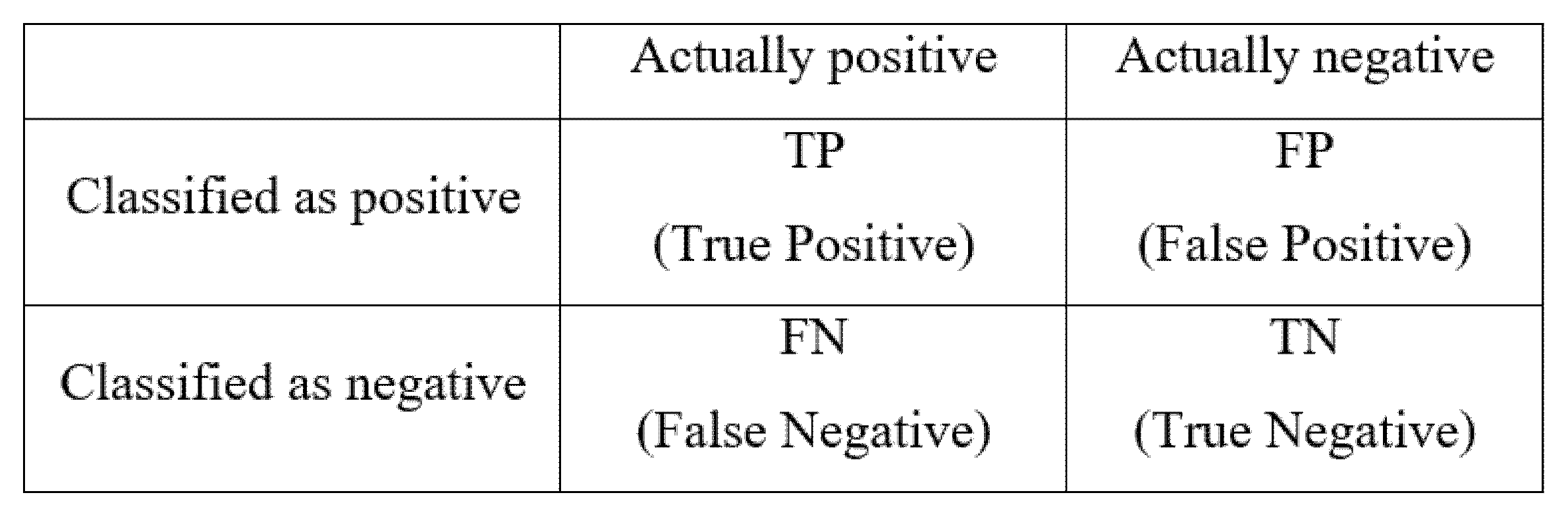
4.1. Temperature Inversion Classification

As described in Section 3.3, CART and CNN were developed to perform the temperature inversion classification. In the machine learning literature, the commonly used measures for evaluating the performance of a two-class (positive or negative) classifier are defined by the confusion matrix as illustrated in Figure 8.

Several useful classification performance metrics such as accuracy, precision, recall, and F1-Score can be evaluated from the confusion matrix as follows.

$$\mathrm{Precision}=\mathrm{TP}/\left(\mathrm{TP}+\mathrm{FP}\right),$$

(3)

$$\mathrm{Recall}=\mathrm{TP}/\left(\mathrm{TP}+\mathrm{FN}\right),$$

(4)

$$\mathrm{Accuracy}=\left(\mathrm{TP}+\mathrm{TN}\right)/\left(\mathrm{TP}+\mathrm{FP}+\mathrm{FN}+\mathrm{TN}\right),$$

(5)

$$\mathrm{F}1-\mathrm{Score}=2\times \mathrm{Precision}\times \mathrm{Recall}/\left(\mathrm{Precision}+\mathrm{Recall}\right).$$

(6)

Each metric gauges the classification performance from a different perspective. Precision focuses on the effectiveness of the samples which the classifier recognizes as positive, while recall emphasizes how many true positive samples are correctly recognized by the classifier. Precision and recall are contrasting measures. A perfect recall can be obtained at the cost of reduced precision by letting the classifier recognize more samples as positive. Accuracy reports the correct recognitions on both positive and negative classes from all test samples. Accuracy could be a biased measure if the data size of the two classes differs significantly. F1-Score is a balanced measure by taking into account both precision and recall simultaneously.

As the time span of our data collected from Taiwan EPA (https://www.epa.gov.tw/ accessed on 10 December 2021) is between 1 January 2016 and 31 December 2019, we used all days in 2016 as the training set for the classifiers and randomly selected 72 test days (two days in each month) from 2017 to 2019 to construct the test set.

Table 1. Comparative performances between CART and CNN for temperature inversion classification.

	2017		2018		2019
	CART	CNN	CART	CNN	CART	CNN
TP	10	11	10	6	9	7
FP	0	2	2	1	0	1
TN	9	7	9	10	12	12
FN	5	4	3	7	3	4
Precision	1.00	0.85	0.83	0.86	1.00	0.88
Recall	0.67	0.73	0.77	0.46	0.75	0.64
Accuracy	0.79	0.75	0.79	0.67	0.88	0.79
F1-Score	0.80	0.79	0.80	0.60	0.86	0.74

shows the comparative performances between CART and CNN. It can be seen that CART outperformed CNN on almost all classification measures across the three test years. The only two exception cases are the recall in 2017 and the precision in 2018. More importantly, CART surpassed CNN in F1-Score for all cases, indicating CART is more suitable than CNN for temperature inversion classification on our dataset.

4.2. PM_2.5 Concentration Estimation

After training the classifiers, namely, CART and CNN, each test day could be firstly labeled as the one with or without temperature inversion. Secondly, the hourly PM_2.5 concentration of the test day was estimated by the regression with the training set according to the test day’s label. If the test day was in the temperature inversion class, the training set including all days with temperature inversion in 2016 was used. Otherwise, a short period of training days immediately prior to the test day was employed as the training set.

To evaluate the accuracy of the PM_2.5 estimation, the performance measures, the rooted mean square error (RMSE) and the mean absolute error (MAE), which have been widely used in the literature, were adopted in this paper and they are defined as follows.

$$\mathrm{RMSE}=\sqrt{{\displaystyle \sum _t{\left(y\left(t\right)-\widehat{y}\left(t\right)\right)}^2}/{\displaystyle \sum _{t}1}},$$

(7)

$$\mathrm{MAE}={\displaystyle \sum _t\left|y\left(t\right)-\widehat{y}\left(t\right)\right|}/{\displaystyle \sum _{t}1},$$

(8)

where t is the duration of test time in number of hours.

Five different forecasting strategies were compared. As noted in Section 3.2, the days in 2016 were manually labeled by experts with two classes, the class with temperature inversion (referred to as Temp_inv) and the class without the phenomenon (referred to as Normal). We noted the results by an expert, which were then used to train CART and CNN, as described in Section 3.3. So we had three classification models (Expert, CART and CNN) which were able to classify a test day into a class (Temp_inv or Normal). For comparison, we further built two dummy classifiers, AllTemp and AllNormal, which always label the test day as Temp_inv or Normal, respectively. The PM_2.5 concentration forecasting was made by multivariate regression as described in Section 3.4. If the test day was classified as Temp_inv by the deployed model, the regression trained on the days in Temp_inv of 2016 was used to make the forecast. Otherwise, the regression trained on a short-term period of days preceding the test day was employed to predict the PM_2.5 concentration.

To verify the best length of the short-term training dataset for forecasting the PM_2.5 of a test day recognized as Normal, we experimented with five, six, and seven days, respectively, to see which training length gives the best performance. The performance of the forecasting results with the test days in the three test years ranging from 2017 to 2019 is tabulated in

Table 2. PM_2.5 forecast performance of various model strategies with short-term training in five days.

		Expert	CART	CNN	AllNormal	AllTemp
2017	RMSE	16.42	16.13	16.32	16.37	16.23
	MAE	12.36	12.29	12.34	12.35	12.4
2018	RMSE	9.01	9.21	9.74	10.37	11.97
	MAE	6.56	6.88	6.87	7.34	8.58
2019	RMSE	7.8	8.59	8.59	8.95	9.7
	MAE	6.05	6.48	6.74	6.77	7.21

,

Table 3. PM_2.5 forecast performance of various model strategies with short-term training in six days.

		Expert	CART	CNN	AllNormal	AllTemp
2017	RMSE	15.68	15.63	15.18	16.02	16.08
	MAE	11.78	11.77	11.39	11.89	12.14
2018	RMSE	8.74	8.99	9.22	10.52	11.59
	MAE	6.65	6.87	6.61	7.77	8.44
2019	RMSE	7.77	8.64	8.61	9.32	8.92
	MAE	5.93	6.55	6.73	7.05	7.21

and

Table 4. PM_2.5 forecast performance of various model strategies with short-term training in seven days.

		Expert	CART	CNN	AllNormal	AllTemp
2017	RMSE	15.01	14.97	14.01	15.32	16.63
	MAE	11.42	11.56	10.63	11.43	13.08
2018	RMSE	7.68	8.18	8.34	8.92	11.24
	MAE	6.33	6.66	7.09	7.16	8.64
2019	RMSE	7.65	7.74	7.56	8.32	8.45
	MAE	5.8	6.27	6.89	6.78	6.85

. Several implications can be drawn from the results. (1) It is noted that the experiments with various length of short-term training dataset only influenced Expert, CART, CNN, and AllNormal. The model AllTemp always refers to the long-term training dataset in 2016 and it will not be affected by varying short-term training length. It is seen that Expert and CART manifest the best performance on all cases when the length of short-term training dataset is set to seven days preceding the test day. Although CNN and AllNormal didn’t always get better results with seven days on all cases, they had the best performance overall with seven-day training dataset. The exceptions were as follows. CNN showed the best MAE result with six days in 2018 and 2019, while AllNormal gave the best 2019 MAE performance when the length of short-term training was set to five days. Considering the overall comparative performances, a seven-day short-term training dataset was employed in our models. (2) In most cases, Expert, CART and CNN outperformed AllNormal and AllTemp on both RMSE and MAE, meaning that the classification of the test day for temperature inversion did improve the performance of the subsequent PM_2.5 forecast. If we compare the mean performance of Expert, CART and CNN, which consider the temperature inversion, to that of AllNormal, the forecast error was reduced by 4~9% and 2~7% in terms of RMSE and MAE. The improvement made by temperature inversion classification was significant. (3) It can be seen that AllNormal surpassed AllTemp on all cases in terms of both RMSE and MAE. This was because the number of days deemed to be under temperature inversion phenomenon was less than one third of all days in the entire year, and AllNormal made more correct classifications than AllTemp and thus obtained better forecast results. (4) It is natural to assume that the forecast assisted by human experts is likely to be superior to that by CART or CNN, because we consider the results of experts as our ground-truth values. This assumption is quite true in 2018 and 2019, but if we look at the forecast result in 2017, CNN makes the best forecasts, while CART and Expert are comparable. With a further investigation, we found that in 2017 Puli township had significantly more pollution days than in 2016, 2018 and 2019. Some of the pollution days were due to external sources instead of temperature inversion as will be noted. These cases incurred large forecast errors for the experts. On the contrary, CART and CNN were not perfect classifiers like Expert; they sometimes misclassified external sources as temperature inversion, which unexpectedly resulted in a better forecast. However, we cannot consider CART and CNN as better classifiers than Expert just based on 2017 results because the Expert was the ground-truth for training the classifiers. The reason for employing CART and CNN was that they can reduce the manual effort of experts labeling the records, and make the recognition of temperature inversion automatic.

One of the typical events caused by external pollutions was on 10 March 2017. We observe there existed a high correlation between the pollution events in Puli and Lunbei (see Figure 3a). Lunbei is near to a large petrochemical complex and it is 65 km southwest of Puli. A river goes between the two townships and forms a potential tunnel for pollution transportation.

Table 5. Relationship between pollution events in Puli and Lunbei.

Hour	Puli PM2.5	Lunbei PM2.5	Wind Speed	Wind Direction
0	51	68	0.0	0
1	53	76	0.6	39
2	48	79	0.9	67
3	46	90	0.3	112
4	44	88	1.2	117
5	41	91	1.2	126
6	41	93	0.0	0
7	44	100	0.0	0
8	46	114	0.4	76
9	48	119	1.0	69
10	56	118	0.9	183
11	53	103	2.2	167
12	46	84	2.0	204
13	41	75	2.5	311
14	33	94	2.4	316
15	33	85	1.8	341
16	54	62	3.1	20
17	96	27	2.7	1
18	123	19	3.3	6
19	126	22	4.0	17
20	127	18	3.6	14
21	127	12	4.1	19
22	124	16	3.6	19
23	116	12	2.8	31

shows the hourly PM_2.5 concentration (μg/m³) for both townships and the wind speeds (m/s) and wind directions (in 360 degrees) observed at Lunbei in the same day. It is seen that the PM_2.5 concentration measured at Lunbei rose since from hour 0 and reached its daily high 119 μg/m³ at hour 9. It then gradually decreased to normal at hour 17. The PM_2.5 concentration measured at Puli showed similar trends but with a time lag of about 10 h. The concentration rose from hour 14 and reached its daily high of 127 μg/m³ at hour 20 and 21. It remained above 100 μg/m³ until midnight. The main wind direction observed at Lunbei during hour 10 and hour 12 was west or southwest with speeds between 0.9 and 2.2 m/s. If we divide the straight distance (65 km) between the two townships by the time lag (10 h), the transportation speed is 1.64 m/s, which is close to the wind speed during the same period. Actually, the transportation speed was a bit higher than 1.64 m/s since the river valley is a curved route, so the two phenomena highly coincided with each other.

The pollution event incurred by external sources definitely cannot be correctly modeled by local climate ecology such as temperature inversion. Our future research will be focused on finding correlated monitoring stations as forecast regulators. For example, the monitoring station at Lunbei may serve as a regulator for the Puli PM_2.5 forecast. If the test day for Puli is classified as normal, then the PM_2.5 measured at Lunbei with some hours ahead (which can be calculated from wind directions and speeds) can be used as an extra variable in the regression to adjust the forecast.

5. Conclusions

In this paper, we have proposed an improved model for PM_2.5 forecasting. The model consists of two phases. In the first phase, a temperature inversion classifier is trained. We chose CART and CNN as the potential classifier for comparison on the Puli dataset. In the second phase, the test day is labeled by the employed classifier as either the temperature inversion class or the other. If it is in the temperature inversion class, the regression trained with the temperature inversion dataset is adopted to make the PM_2.5 forecast. Otherwise, the regression trained with the seven days prior to the test day is used to predict the PM_2.5 concentration. The experimental results show that CART outperforms CNN for temperature inversion classification on the Puli dataset. With the classifiers, the test day for PM_2.5 forecast is subject to the regression trained with the correct class. The forecast experiments tested on the Puli meteorology dataset during 2017 to 2019 show that the models considering the temperature inversion factor can reduce the forecast errors by 4–9% and 2–7% in terms of RMSE and MAE, as compared to the original model. However, there are some limitations regarding this research. The main meteorological patterns leading to temperature inversion vary from place to place. The classifier should be retrained with the dataset collected for the investigated location. Furthermore, our current forecast model based on temperature inversion classification may under-forecast PM_2.5 when external pollution sources arise. Our future research is directed to finding correlated PM_2.5 monitoring stations along the pollution transportation route as forecast regulators to adjust our model.

References

1. Song, C.; He, J.; Wu, L.; Jin, T.; Chen, X.; Li, R.; Ren, P.; Zhang, L.; Mao, H. Health burden attributable to ambient PM2.5 in China. Environ. Pollut. 2017, 223, 575–586. [Google Scholar] [CrossRef] [PubMed]
2. Chen, Y.C.; Chiang, H.C.; Hsu, C.Y.; Yang, T.T.; Lin, T.Y.; Chen, M.J.; Chen, N.T.; Wu, Y.S. Ambient PM2.5-bound polycyclic aromatic hydrocarbons (PAHs) in Changhua County, Central Taiwan: Seasonal variation, source apportionment and cancer risk assessment. Environ. Pollut. 2016, 218, 372–382. [Google Scholar] [CrossRef]
3. WHO Media Centre, Ambient (Outdoor) Air Quality and Health. Available online: http://www.who.int/mediacentre/factsheets/fs313/en/ (accessed on 30 October 2019).
4. Liang, C.S.; Duan, F.K.; He, K.B.; Ma, Y.L. Review on recent progress in observations, source identifications and countermeasures of PM2.5. Environ. Int. 2016, 86, 150–170. [Google Scholar] [CrossRef]
5. Singh, N.; Murari, V.; Kumar, M.; Barman, S.C.; Banerjee, T. Fine particulates over South Asia: Review and meta-analysis of PM2.5 source apportionment through receptor model. Environ. Pollut. 2017, 223, 121–136. [Google Scholar] [CrossRef] [PubMed]
6. Hsu, C.H.; Cheng, F.Y. Classification of weather patterns to study the influence of meteorological characteristics on PM2.5 concentrations in Yunlin County, Taiwan. Atmos. Environ. 2016, 144, 397–408. [Google Scholar] [CrossRef]
7. Chen, M.L.; Mao, I.F.; Lin, I.K. The PM2.5 and PM10 particles in urban areas of Taiwan. Sci. Total Environ. 1999, 226, 227–235. [Google Scholar] [CrossRef]
8. Hsu, C.Y.; Chiang, H.C.; Lin, S.L.; Chen, M.J.; Lin, T.Y.; Chen, Y.C. Elemental characterization and source apportionment of PM10 and PM2.5 in the western coastal area of central Taiwan. Sci. Total Environ. 2016, 541, 1139–1150. [Google Scholar] [CrossRef]
9. Kuo, Y.M.; Wang, S.W.; Jang, C.S.; Yeh, N.; Yu, H.L. Identifying the factors influencing PM2.5 in southern Taiwan using dynamic factor analysis. Atmos. Environ. 2011, 45, 7276–7285. [Google Scholar] [CrossRef]
10. Hwang, S.L.; Lin, Y.C.; Guo, S.E.; Chi, M.C.; Chou, C.T.; Lin, C.M. Emergency room visits for respiratory diseases associated with ambient fine particulate matter in Taiwan in 2012: A population-based study. Atmos. Pollut. Res. 2017, 8, 465–473. [Google Scholar] [CrossRef]
11. Chen, L.J.; Ho, Y.H.; Lee, H.C.; Wu, H.C.; Liu, H.M.; Hsieh, H.H.; Huang, Y.T.; Lung, S.C. An open framework for participatory PM2.5 monitoring in smart cities. IEEE Access 2017, 5, 14441–14454. [Google Scholar] [CrossRef]
12. Tsai, Y.I.; Sopajaree, K.; Kuo, S.C.; Yu, S.P. Potential PM2.5 impacts of festival-related burning and other inputs on air quality in an urban area of southern Taiwan. Sci. Total Environ. 2015, 527, 65–79. [Google Scholar] [CrossRef]
13. Chuang, M.T.; Chang, S.C.; Lin, N.H.; Wang, J.L.; Sheu, G.R.; Chang, Y.J.; Lee, C.T. Aerosol chemical properties and related pollutants measured in Dongsha Island in the northern South China Sea during 7-SEAS/Dongsha experiment. Atmos. Environ. 2013, 78, 82–92. [Google Scholar] [CrossRef]
14. Yu, H.L.; Chien, L.C.; Yang, C.H. Asian dust storm elevates children’s respiratory health risks: A spatiotemporal analysis of children’s clinic visits across Taipei (Taiwan). PLoS ONE 2012, 7, e41317. [Google Scholar] [CrossRef] [Green Version]
15. Xu, L.; Yu, Y.; Yu, J.; Chen, J.; Niu, Z.; Yin, L.; Zhang, F.; Liao, X.; Chen, Y. Spatial distribution and sources identification of elements in PM2.5 among the coastal city group in the western Taiwan Strait region, China. Sci. Total Environ. 2013, 442, 77–85. [Google Scholar]
16. Triantafyllou, A.G.; Kiros, E.S.; Evagelopoulos, V.G. Respirable particulate matter at an urban and nearby industrial location: Concentrations and variability and synoptic weather conditions during high pollution episodes. J. Air Waste Manag. Assoc. 2002, 52, 287–296. [Google Scholar] [CrossRef] [PubMed] [Green Version]
17. Gramsch, E.; Cáceres, D.; Oyola, P.; Reyes, F.; Vásquez, Y.; Rubio, M.A.; Sánchez, G. Influence of surface and subsidence thermal inversion on PM2.5 and black carbon concentration. Atmos. Environ. 2014, 98, 290–298. [Google Scholar] [CrossRef]
18. Wallace, J.; Kanaroglou, P. The effect of temperature inversions on ground-level nitrogen dioxide (NO2) and fine particulate matter (PM2.5) using temperature profiles from the Atmospheric Infrared Sounder (AIRS). Sci. Total Environ. 2009, 407, 5085–5095. [Google Scholar] [CrossRef]
19. Tran, H.N.Q.; Mölders, N. Investigations on meteorological conditions for elevated PM2.5 in Fairbanks, Alaska. Atmos. Res. 2011, 99, 39–49. [Google Scholar] [CrossRef]
20. Vlachogianni, A.; Kassomenos, P.; Karppinen, A.; Karakitsios, S.; Kukkonen, J. Evaluation of a multiple regression model for the forecasting of the concentrations of NOx and PM10 in Athens and Helsinki. Sci. Total Environ. 2011, 409, 1559–1571. [Google Scholar] [CrossRef] [PubMed]
21. Moisan, S.; Herrera, R.; Clements, A. A dynamic multiple equation approach for forecasting PM2.5 pollution in Santiago, Chile. Int. J. Forecast. 2018, 34, 566–581. [Google Scholar] [CrossRef] [Green Version]
22. Zhang, T.; Liu, P.; Sun, X.; Zhang, C.; Wang, M.; Xu, J.; Pu, S.; Huang, L. Application of an advanced spatiotemporal model for PM2.5 prediction in Jiangsu Province, China. Chemosphere 2020, 246, 125563. [Google Scholar] [CrossRef] [PubMed]
23. Cobourn, W.G. An enhanced PM2.5 air quality forecast model based on nonlinear regression and back-trajectory concentrations. Atmos. Environ. 2010, 44, 3015–3023. [Google Scholar] [CrossRef]
24. Baker, K.R.; Foley, K.M. A nonlinear regression model estimating single source concentrations of primary and secondarily formed PM2.5. Atmos. Environ. 2011, 45, 3758–3767. [Google Scholar] [CrossRef]
25. Yin, Q.; Wang, J.; Hu, M.; Wong, H. Estimation of daily PM2.5 concentration and its relationship with meteorological conditions in Beijing. J. Environ. Sci. 2016, 48, 161–168. [Google Scholar] [CrossRef]
26. Ni, X.Y.; Huang, H.; Du, W.P. Relevance analysis and short-term prediction of PM2.5 concentrations in Beijing based on multi-source data. Atmos. Environ. 2017, 150, 146–161. [Google Scholar] [CrossRef]
27. Wang, P.; Zhang, H.; Qin, Z.; Zhang, G. A novel hybrid-Garch model based on ARIMA and SVM for PM2.5 concentrations forecasting. Atmos. Pollut. Res. 2017, 8, 850–860. [Google Scholar] [CrossRef]
28. Mogollón-Sotelo, C.; Casallas, A.; Vidal, S. A support vector machine model to forecast ground-level PM2.5 in a highly populated city with a complex terrain. Air Qual. Atmos. Health 2021, 14, 399–409. [Google Scholar] [CrossRef]
29. Liu, W.; Guo, G.; Chen, F.; Chen, Y. Meteorological pattern analysis assisted daily PM2.5 grades prediction using SVM optimized by PSO algorithm. Atmos. Pollut. Res. 2019, 10, 1482–1491. [Google Scholar] [CrossRef]
30. Mao, X.; Shen, T.; Feng, X. Prediction of hourly ground level PM2.5 concentrations 3 days in advance using neural networks with satellite data in eastern China. Atmos. Pollut. Res. 2017, 8, 1005–1015. [Google Scholar] [CrossRef]
31. Di, Q.; Amini, H.; Shi, L.; Kloog, I.; Silvern, R.; Kelly, J.; Sabath, M.B.; Choirat, C.; Koutrakis, P.; Lyapusting, A.; et al. An ensemble-based model of PM2.5 concentration across the contiguous United States with high spatiotemporal resolution. Environ. Int. 2019, 130, 104909. [Google Scholar] [CrossRef]
32. Xiao, F.; Yang, M.; Fan, H.; Fan, G.; Al-qaness, M.A.A. An improved deep learning model for predicting daily PM2.5 concentration. Sci. Rep. 2020, 10, 20988. [Google Scholar] [CrossRef] [PubMed]
33. Qin, D.; Yun, J.; Zou, G.; Yong, R.; Zhao, Q.; Zhang, B. A novel combined prediction scheme based on CNN and LSTM for urban PM25 concentration. IEEE Access 2019, 7, 20050–20059. [Google Scholar] [CrossRef]
34. Zhang, B.; Li, X.; Zhao, Y.; Li, Y.; Wang, X. Air quality PM2.5 prediction based on multi-model fusion. In Proceedings of the 2019 Chinese Control and Decision Conference (CCDC), Nanchang, China, 3–5 June 2019. [Google Scholar]
35. Breiman, L.; Friedman, J.H.; Olshen, R.A.; Stone, C.J. Classification and Regression Trees; Wadsworth & Brooks/Cole Advanced Books & Software: Monterey, CA, USA, 1984. [Google Scholar]
36. LeCun, Y.; Haffner, P.; Bottou, L.; Bengio, Y. Object recognition with gradient-based learning. In Shape, Contour and Grouping in Computer Vision; Lecture Notes in Computer Science; Springer: Berlin/Heidelberg, Germany, 1999; Volume 1681. [Google Scholar]
37. Krizhevsky, A.; Sutskever, I.; Hinton, G.E. ImageNet classification with deep convolutional neural networks. Adv. Neural Inf. Process. Syst. 2012, 25, 1097–1105. [Google Scholar] [CrossRef]
38. Szegedy, C.; Liu, W.; Jia, Y.; Sermanet, P.; Reed, S.; Anguelov, D.; Erhan, D.; Vanhoucke, V.; Rabinovich, A. Going deeper with convolutions. In Proceedings of the 2015 IEEE Conference on Computer Vision and Pattern Recognition (CVPR), Boston, MA, USA, 7–12 June 2015. [Google Scholar] [CrossRef] [Green Version]
39. He, K.; Zhang, X.; Ren, S.; Sun, J. Deep residual learning for image recognition. In Proceedings of the 2016 IEEE Conference on Computer Vision and Pattern Recognition (CVPR), Las Vegas, NV, USA, 26 June–1 July 2016; pp. 770–778. [Google Scholar] [CrossRef] [Green Version]
40. Hu, J.; Shen, L.; Sun, G. Squeeze-and-excitation networks. In Proceedings of the 2018 IEEE Conference on Computer Vision and Pattern Recognition (CVPR), Salt Lake City, UT, USA, 18–23 June 2018. [Google Scholar] [CrossRef] [Green Version]
41. Clerc, M.; Kennedy, J. The particle swarm explosion, stability, and convergence in a multidimensional complex space. IEEE Trans. Evol. Comput. 2002, 6, 58–73. [Google Scholar] [CrossRef] [Green Version]
Figure 1. Temperature inversion. (a) Normal aerosol convection; (b) inhibited aerosol convection under the warm air inversion layer.
Applsci 12 00071 g001
Figure 2. Relationship between temperature and PM2.5 concentrations observed at Puli EPA supersite. (a) Entire year 2016 with a different color for each season; (b) summer; (c) autumn.
Applsci 12 00071 g002
Figure 3. The investigated site. (a) Location of Puli township and two potential external pollution sources. (b) Geography of Puli township and the Taiwan EPA supersite (located at the Puli middle school).
Applsci 12 00071 g003
Figure 4. The data labeling for two plausible examples of temperature inversion phenomena.
Applsci 12 00071 g004
Figure 5. The mean hourly PM2.5 value observed at Puli EPA supersite for the days with or without the plausible meteorological phenomena causing temperature inversion.
Applsci 12 00071 g005
Figure 6. The learned decision tree from the collected data in 2016.
Applsci 12 00071 g006
Figure 7. The learning curve of our CNN model with the training set and validation set.
Applsci 12 00071 g007
Figure 8. Confusion matrix.
Applsci 12 00071 g008