Prediction and Analysis of the Surface Roughness in CNC End Milling Using Neural Networks

Abstract

In the metal cutting process of machine tools, the quality of the surface roughness of the product is very important to improve the friction performance, corrosion resistance, and aesthetics of the product. Therefore, low surface roughness is ideal for mechanical cutting. If the surface roughness of the product can be predicted, not only the quality of the product can be improved but also the processing cost can be reduced. In this study a back propagation neural network (BPNN) was proposed to predict the surface roughness of the processed workpiece. ANOVA was used to analyze the influence of milling parameters, such as spindle speed, feed rate, cutting depth, and milling distance. The experimental results show that the root mean square error (RMSE) obtained by using the back propagation neural network is 0.008, which is much smaller than the 0.021 obtained by the traditional linear regression method.

1. Introduction

In metal cutting, the workpiece quality obtained by different machining parameters is also different. In the processing of the spindle, speed is fast and slow, the feed is high and low; in the processing of the chip, there are many factors affecting the final quality of the workpiece [1,2,3,4]. The back propagation neural network is used to detect the surface roughness [5]. Bit diameter, cutting speed, feed and processing time are used as inputs to the neural network structure, and the surface roughness is estimated. Design of Experiment (DOE) is a method to arrange the contents of the experiment and analyze the experimental data by using optimal words. This method has a wide range of applications, including production process and equipment parameters, process methods, raw materials, or formula selection, to improve product quality or output [6,7].

There are many ways to predict surface roughness and analyze each machining parameter. At present, the common prediction method is to establish the prediction model by using the method of neural network [8,9,10,11]. Zain et al. [12] present the Artificial Neural Network (ANN) model for predicting the surface roughness performance measure in the machining process by considering the ANN as the essential technique for measuring surface roughness. In the prediction of surface roughness, different processing parameters can be used as input to neural networks [13,14,15,16,17,18,19,20]. Zerti et al. [21] used the response surface methodology and the artificial neural networks approach for output modeling. The method of parametric analysis is also useful to analyze by many statistical methods. Surface roughness is not only an output but also an input to predict other processing parameters in neural networks. Thangarasu et al. [22], based on the response of cutting force and surface roughness, used artificial neural network to predict the side wear of cutting tools.

In this study, the machining method of milling was used for experiments, and the prediction was made by using the back propagation neural network, in which the input parameters were cutting depth, spindle speed, feed, milling pitch, and the output was the surface roughness of the workpiece. Linear regression was used to compare the root mean square error (RMSE) and ANOVA was used to analyze the relationship between parameters, and the influence of input parameters of output was discussed. In this study, the inverse transfer neural network was used for modeling. The input parameters were cutting depth, feed, spindle speed, milling pitch, and the output was workpiece surface roughness.

The remainder of this study is organized as follows. Section 2 describes the prediction and analysis of the surface roughness, Section 3 presents the results and discussion, and the Section 4 offers conclusions for this study.

2. Prediction and Analysis of the Surface Roughness

2.1. Surface Roughness and Experimental Setup

The surface of any processed part has a complex structure with numerous ridges and depressions with different heights, depths, and gaps. Surface roughness refers to the small gaps in the surface of the high and low frequency of the formation of a depression. Surface roughness affects the amount of wear and tightness of parts when they engage with other objects. For all of these reasons, the need to numerically manage surface nuances has increased in recent years.

Figure 1 depicts the waveform of surface roughness. A baseline is presented in the figure as a reference. The surface roughness has irregular peaks and valleys.

Figure 2 depicts the contour curve of the arithmetic average height. The arithmetic average height represents the average of the absolute value of the base length.

When the contour curve depicts the roughness curve, Ra is called the arithmetic mean roughness; when the contour curve depicts the waviness curve, $W_a$ is called arithmetic mean waviness. Equation (1) is the mathematical formula of arithmetic average height. Ra was used the reference value.

$$Ra=\frac{1}{lr}\int \begin{array}{c}lr\\ 0\end{array}\left|Z\left(x\right)\right|\mathrm{dx}$$

(1)

where lr is benchmark length and $Ra$ is the arithmetic average height. A section of the reference length is sampled from the average direction of the roughness curve, and the X-axis and Y-axis are set in the sampling part of the mean line. When the roughness curve Y = Z(x), the values of $Ra$ is obtained by formula x in microns (μm).

The S220 CEXSH31000 micro grain carbide end milling tool (CMTec) was used in this study. The specifications of the tool are presented in

Table 1. Tool S220 specifications.

Blade Diameter (d)	Blade Length (L1)	Tool Length (L)	Number of Edges (F)	Helix Angle
10 (mm)	30 (mm)	75 (mm)	3	45°

.

Four parameters, feed rate, spindle speed, cutting depth, and milling pitch, were evaluated in this study. The experiment was a three layer experiment. A total of 54 experiments were conducted. The recommended parameters for milling aluminum work pieces are presented in

Table 2. S220 CEXSH31000 end mills milling parameter recommended value.

Spindle Speed	Feed	$\mathbf{Cutting} \mathbf{Depth} \left({\mathit{d}}_{\mathit{c}}\right)$	$\mathbf{Cutting} \mathbf{Width} \left({\mathit{d}}_{\mathit{w}}\right)$
5760 (rpm)	1260 (mm/min)	1.5 (mm)	0.1 (mm)

. The configuration of experimental parameters is depicted in

Table 3. Experimental parameter configuration.

	1 Layer	2 Layer	3 Layer
Feed (mm/min)	3000	4000	5000
Spindle speed(rpm)	3000	5000	8000
Cutting depth (mm)	0.5	1	1.5
Milling pitch (mm)	3	5

.

The MF400U Quaser five-axis vertical machining center was used in the experiment. The specifications of the machine are listed in

Table 4. Quaser five-axis vertical machining center MF400U.

Item	Parameter
Workbench size (mm)	$\varphi$320
Maximum workpiece rotation diameter (mm)	$\varphi$400
Maximum workpiece size (mm)	$\varphi$400 × 300
Workbench load (kg)	100
X-axis (mm)	410
Y-axis (mm)	610
Z-axis (mm)	510
A-axis	+30°~120°
C-axis	360°
Maximum spindle speed (rpm)	10,000
Controller	SIEMENS

.

2.2. BPNN

The BPNN is a multi-layer feedforward network with learning ability and is used to train an ANN; it includes at least three layers (input layer, hidden layer, and output layer). The BPNN is a supervised learning network. The training data and the target output data are input into the neural network, and the weights are adjusted repeatedly by using the steepest (a type of gradient descent) method to minimize the error between the neural network output and the actual value. Herein, we present theoretical and mathematical derivations of the BPNN. The BPNN is implemented as follows.

First, determine the input layer neurons $x_m$, the number of hidden layer neurons $h_o$, and number of output layer neurons $y_n$.

Then, the bias between the weight value and the neural network is randomly set. $w_{ij}$ is the weights between the input layer and hidden layer. $w_{jk}$ is the weights between hidden layer and output layer. The deviation of $\theta h_o$ is hidden layer. ${\theta }_{yn}$ is biased output layer.

To calculate the output value of the hidden layer the formula is as follows:

$$net\_h_O={\displaystyle \sum }_{m=1}^M{w}_{ij}\times x_m-\theta h_o$$

(2)

$$h_o=\frac{1}{1+e^{-net\_h_0}}$$

(3)

where net$\_h_O$ is the product of the number of neurons in the hidden layer weighted sum, M; is the total number of input layer neurons, and the output value is the number of neurons in the hidden layer, and the nonlinear transform.

For the output value of the output layer the formula is as follows:

$$net\_y_n={\displaystyle \sum }_{o=1}^O{w}_{jk}\times h_o-\theta y_n$$

(4)

$$y_n=\frac{1}{1+e^{-net\_y_n}}$$

(5)

where net$\_y_n$ is the product of the number of neurons in output layer weighted sum, O is the total number of hidden layer neurons, and $y_n$ is the neural network output value.

For the error amount of the output layer the formula is as follows.

$$\mathsf{\Delta }{y}_n=y_n·\left(1-y_n\right)·\left(T_n-y_n\right)$$

(6)

where the delta $\delta y_n$ error volume is the number of neurons in the output layer; $y_n$ and between the amount of error. $T_n$ output value as the goal.

The error of the hidden layer the formula is calculated as follows.

$$\delta h_o=h_o·\left(1-h_o\right)·{\displaystyle \sum }_{n=1}^N{w}_{jk}·\delta y_n$$

(7)

where $\delta h_o$ denotes the number of neurons in the hidden, and the N is the total number of output layer neurons.

For the weight value between the input layer and the hidden layer, the formula is as follows.

$$w_{ij}=w_{ij}+\Delta w_{ij}$$

(8)

To calculate the deviation value of the hidden layer the formula is as follows.

$$\theta h_o=\theta h_o+\Delta \theta h_o$$

(9)

For the weight value between the hidden layer and the output layer, the formula is as follows.

$$w_{jk}=w_{jk}+\Delta w_{jk}$$

(10)

The offset value of the output layer is updated as follows.

$$\theta y_n=\theta y_n+\Delta \theta y_n$$

(11)

The squared error of the output neuron is calculated as follows.

$$E=\frac{1}{2}{\displaystyle \sum }_n{(T_n-y_n)}^2$$

(12)

where E is the square error of the output neurons, $T_n$ is the target output value, and $Y_n$ is the neural network output value. After one learning cycle, if the error obtained is smaller, the performance of neural network learning is better. The smaller the error between the output value of the neural network and the target output value is, the better.

According to Table 2, we designed the orthogonal table of L24. The training data of the BPNN are depicted in

Table 5. Experimental orthogonal table.

No.	Cutting Depth (mm)	Spindle Speed (rpm)	Feed (mm/min)	Milling Pitch (mm)	Ra ($\mathsf{\mu }\mathbf{m}$)
1	0.5	3000	3000	0.3	1.895
2	0.5	3000	4000	0.3	2.729
3	0.5	3000	5000	0.3	3.337
4	0.5	3000	3000	0.5	2.027
5	0.5	3000	4000	0.5	2.700
6	0.5	3000	5000	0.5	3.487
7	0.5	5000	3000	0.3	1.386
8	0.5	5000	4000	0.3	1.517
9	0.5	5000	5000	0.3	1.645
10	0.5	5000	3000	0.5	1.416
11	0.5	5000	4000	0.5	1.903
12	0.5	5000	5000	0.5	2.249
13	0.5	8000	3000	0.3	1.354
14	0.5	8000	4000	0.3	1.377
15	0.5	8000	5000	0.3	1.520
16	0.5	8000	3000	0.5	1.523
17	0.5	8000	4000	0.5	1.425
18	0.5	8000	5000	0.5	1.439
19	1	3000	3000	0.3	2.455
20	1	3000	4000	0.3	2.959
21	1	3000	5000	0.3	4.070
22	1	3000	3000	0.5	3.378
23	1	3000	4000	0.5	4.191
24	1	3000	5000	0.5	3.721
25	1	5000	3000	0.3	2.221
26	1	5000	4000	0.3	2.717
27	1	5000	5000	0.3	2.483
28	1	5000	3000	0.5	1.612
29	1	5000	4000	0.5	2.105
30	1	5000	5000	0.5	2.476
31	1	8000	3000	0.3	1.683
32	1	8000	4000	0.3	2.049
33	1	8000	5000	0.3	2.336
34	1	8000	3000	0.5	1.395
35	1	8000	4000	0.5	1.731
36	1	8000	5000	0.5	2.069
37	1.5	3000	3000	0.3	2.801
38	1.5	3000	4000	0.3	3.813
39	1.5	3000	5000	0.3	4.461
40	1.5	3000	3000	0.5	3.018
41	1.5	3000	4000	0.5	5.509
42	1.5	3000	5000	0.5	23.901
43	1.5	5000	3000	0.3	3.005
44	1.5	5000	4000	0.3	2.838
45	1.5	5000	5000	0.3	3.617
46	1.5	5000	3000	0.5	2.722
47	1.5	5000	4000	0.5	2.883
48	1.5	5000	5000	0.5	3.586
49	1.5	8000	3000	0.3	1.534
50	1.5	8000	4000	0.3	1.969
51	1.5	8000	5000	0.3	3.043
52	1.5	8000	3000	0.5	1.312
53	1.5	8000	4000	0.5	2.469
54	1.5	8000	5000	0.5	2.663

. A total of 54 data experiments were conducted. The 42nd group of data produced extreme data because of the relationship between the rotational speed and feed rate.

2.3. Analysis of Variance

Analysis of variance (ANOVA) was used to evaluate continuous and dependent variables. Furthermore, for the variables (independent variable), when the variable factors were contained in the equal to or more than three categories, we checked whether the average between all kinds did not equal statistical models

The three main assumptions of ANOVA are as follows:

• The ethnic distributions implied by each group of samples must be normal or approximately normal.
• Each group of samples must be independent.
• The number of ethnic variations must be equal.

The values required for ANOVA are summarized in

Table 6. ANOVA table.

	Sum of Square (SS)	Degree of Freedom (DF)	Mean of Square (MS)	F (Test)	p-Value
Between group	$S{S}_B$	$G-1$ (Group-1)	$M{S}_{\mathrm{B}}$	$\frac{M{S}_B}{M{S}_W}$	Table search
Within group	$S{S}_W$	$\left(N-1\right)-\left(G-1\right)$ $=N-G$	$M{S}_{\mathrm{W}}$
Total	$S{S}_T$	$N-1$ (Samples-1)

, where Total Sum of Square Error: $S{S}_T$, Between Group Sum of Square Error: $S{S}_B$, Between Group Mean of Square Error: $M{S}_B$, Within Group Mean of Square Error: $M{S}_w$.

3. Results and Analysis

3.1. Effect of Input Parameters on Surface Roughness

According to the results, the influence of the cutting parameters on surface roughness can be categorized into two states. In the first state, one parameter is mutable and the other two parameters are constant. In the second state, the two parameters are interactive, and one parameter is constant. Thus, the surface roughness can be observed through the changes of the two parameters, leaving the other parameters unchanged. Figure 3, Figure 4, Figure 5 and Figure 6 depict the influence of four input parameters on surface roughness.

From Figure 3, Figure 4, Figure 5 and Figure 6, it can be found that the smaller the cutting depth, the smaller the surface roughness measured. If the spindle speed gets faster, the surface roughness of the workpiece gets smaller. The smaller the feed rate, the smaller the surface roughness. In the milling spacing diagram, we find that the smaller the milling spacing, the smaller the surface roughness.

3.2. Results of ANOVA

ANOVA is a standard statistical tool for determining the effects of a single parameter from all input process parameters. In this analysis, the percentage contribution of each parameter is used to measure its corresponding effect on the output response. In this study, ANOVA was used to analyze the influence of milling parameters, that is, spindle speed, feed rate, cutting depth, and milling spacing will affect the surface roughness.

Table 7. ANOVA results for the cutting depth.

	SS	DF	MS	F	p-Value	Critical Value	Con (%)
$S{S}_B$	59.3598	1	59.3598	112.0691	<0.0001	3.932438	51.86%
$S{S}_w$	55.08584	104	0.529672
$S{S}_T$	114.4456	105

,

Table 8. ANOVA results for the spindle speed.

	SS	DF	MS	F	p-Value	Critical Value	Con (%)
$S{S}_B$	7.66 × 108	1	7.66 × 108	357.9129	<0.0001	3.932438	77.48%
$S{S}_w$	2.22 × 108	104	2,138,970
$S{S}_T$	9.88 × 108	105

,

Table 9. ANOVA results for the feed.

	SS	DF	MS	F	p-Value	Critical Value	Con (%)
$S{S}_B$	4.19 × 108	1	4.19 × 108	1247.14	<0.0001	3.932438	92.3%
$S{S}_w$	3.49 × 107	104	336,357.5
$S{S}_T$	4.54 × 108	105

and

Table 10. ANOVA results for the milling pitch.

	SS	DF	MS	F	p-Value	Critical Value	Con (%)
$S{S}_B$	115.6564	1	115.6564	256.6285	<0.0001	3.932438	71%
$S{S}_w$	46.87036	104	0.450677
$S{S}_T$	162.5268	105

list ANOVA results for surface roughness and four input parameters.

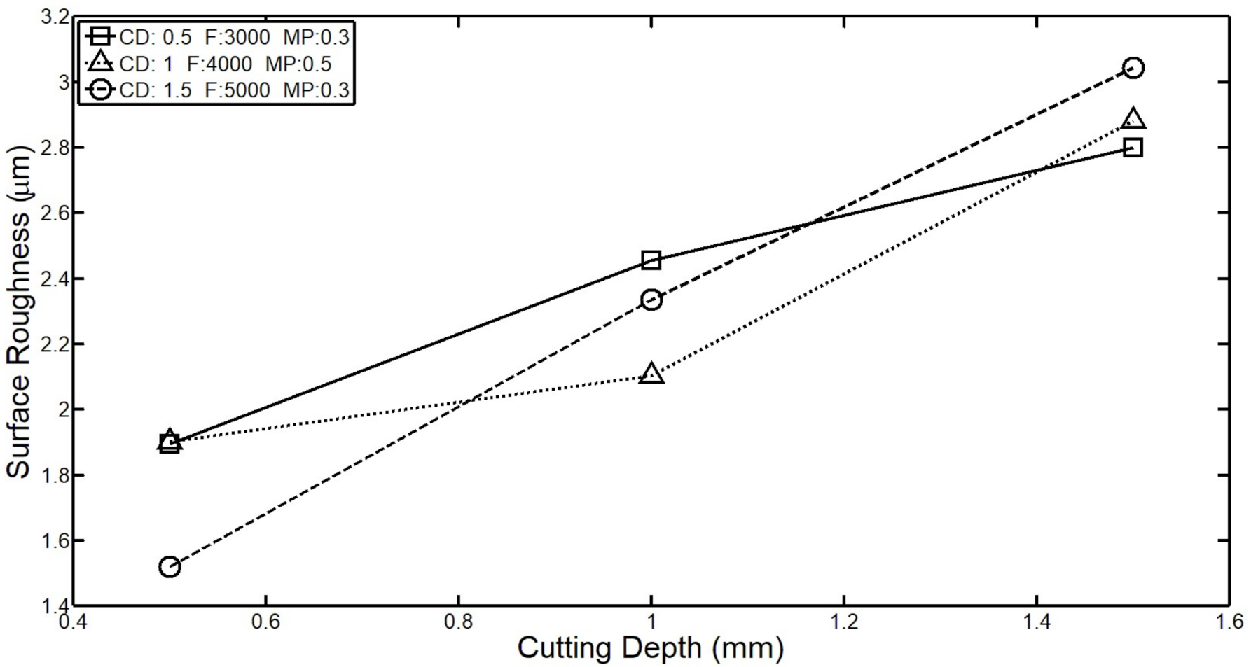
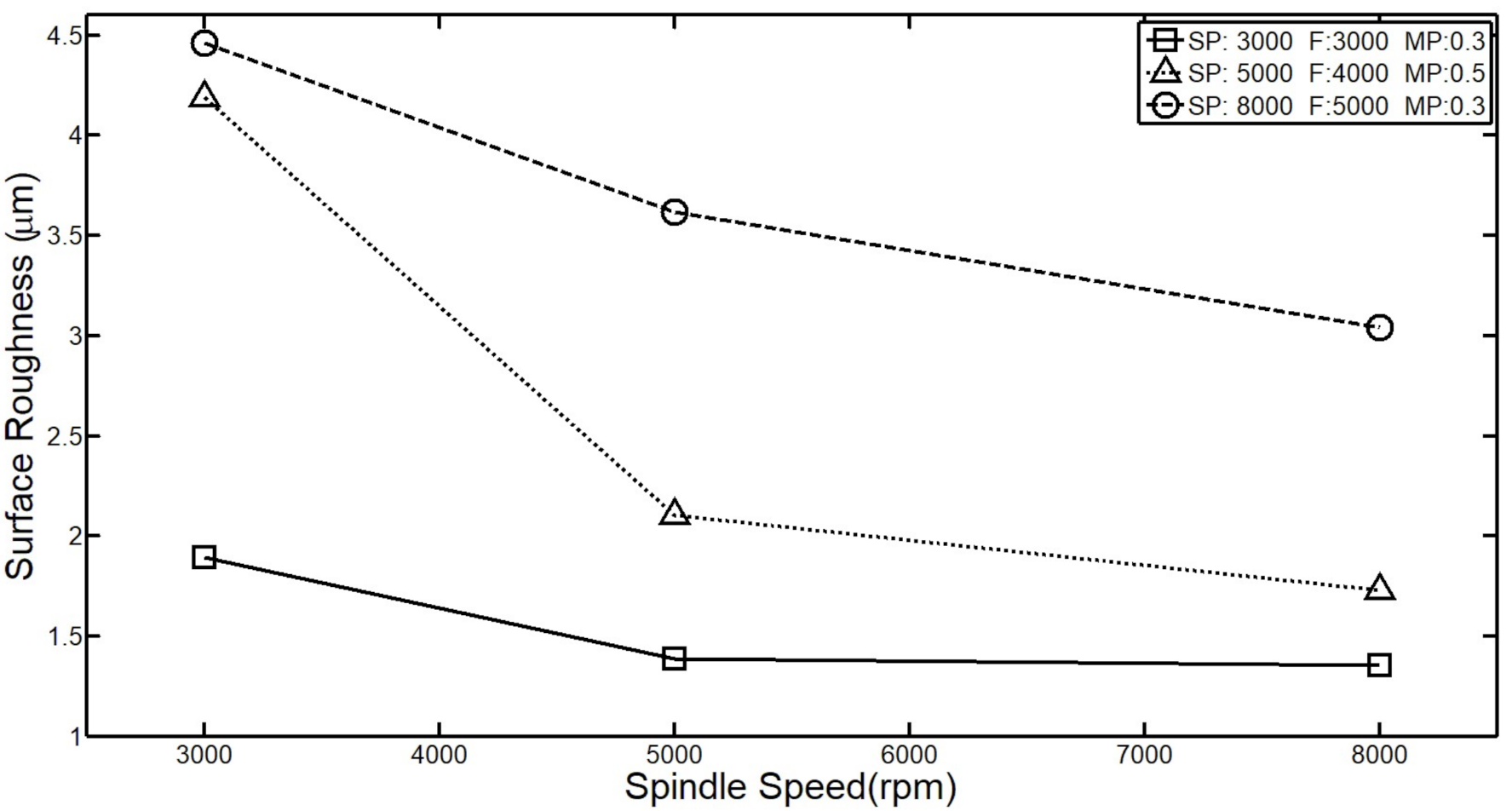
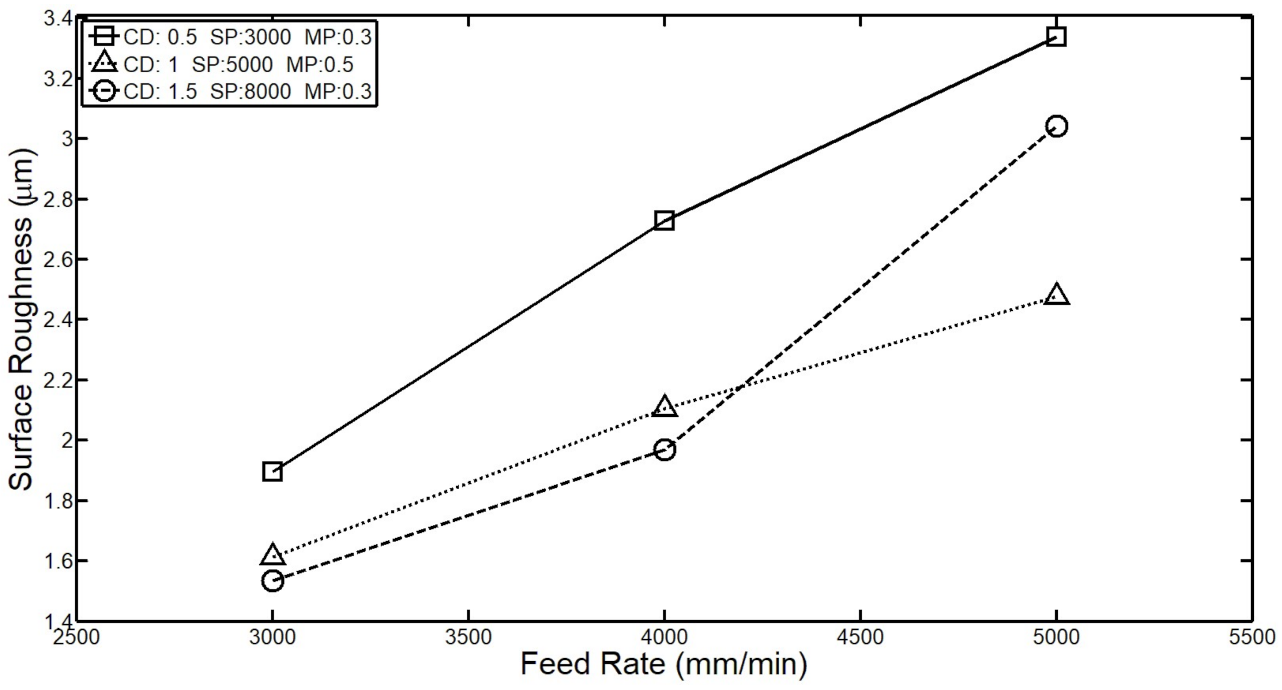
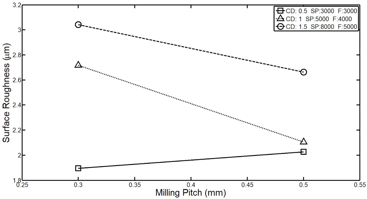
For the cutting depth, spindle speed, feed rate, and milling distance, p-values are far less than 0.0001, which means that these four processing parameters and surface roughness have a first relation. The main contribution of cutting depth was 51.86%. The contribution of spindle speed was 77.48%. The contribution of feed was 92.3%. The contribution of milling spacing was 71%. ANOVA statistics show that the cutting depth is a parameter with low contribution. From the value of F, it was found that the model is meaningful. In general, surface roughness is measured as a function of feed speed. Therefore, it has the physical significance and the greatest contribution. The contribution of spindle speed and milling spacing is similar.

3.3. Parameter Analysis of BPNN

The back propagation neural network is a multi-layer feedforward network with learning ability. It is a method to train the artificial neural network, including at least three layers (input layer, hidden layer, and output layer). Its learning is a kind of supervised learning. The training data and the target output data were input into the neural network, and the weights were adjusted repeatedly by using the gradient steepest descent method to minimize the error between the neural network output and the actual value. Next, we will introduce the theory and mathematical derivation of back propagation neural networks.

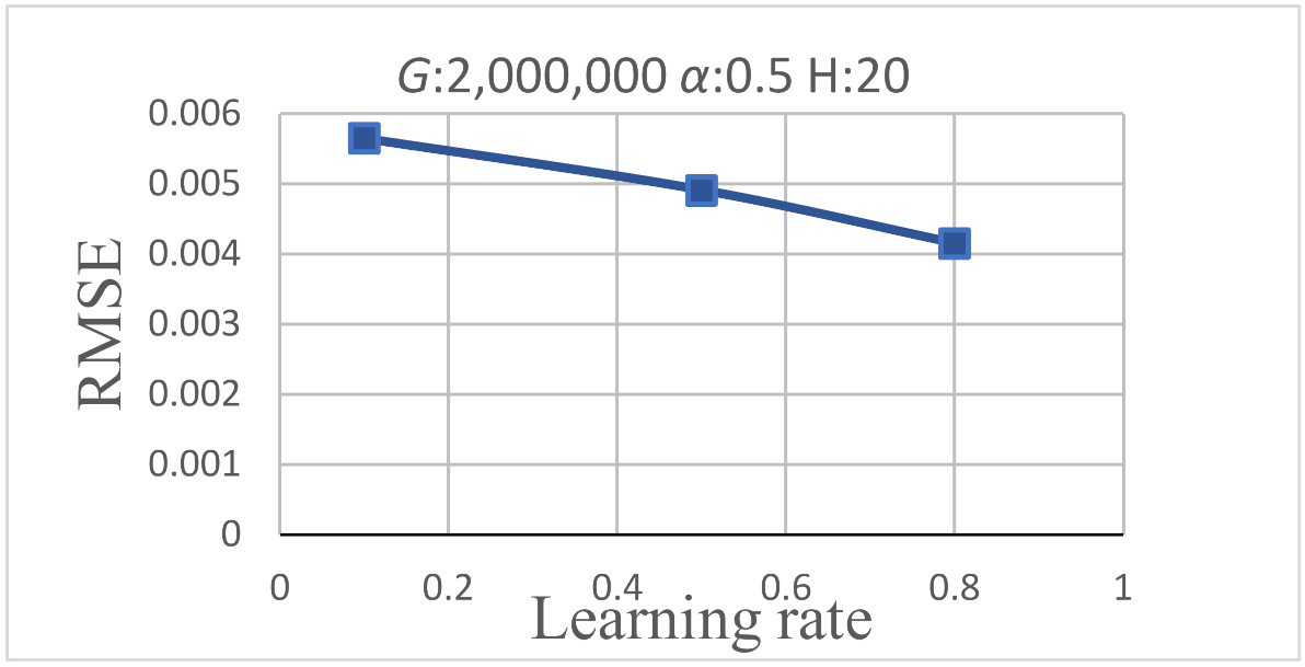
When the learning rate is too small, it can avoid network vibration. However, this phenomenon leads to slow convergence, which results in a slow learning rate. If the learning rate is too large, the target value can be approached faster. However, too much correction can result in network vibration, or even lead to network weight value divergence.

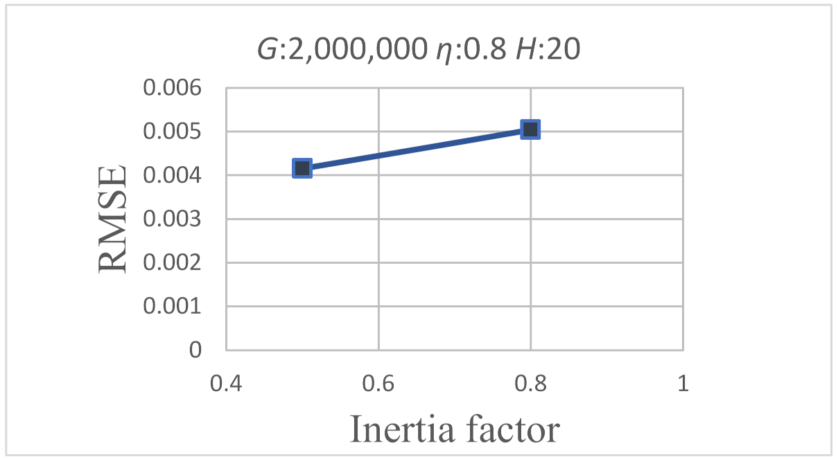
The inertia factor is the change from the previous weighted value to the next weighted value. Typically, the value is between 0 and 1. The weights should be moved in the same direction.

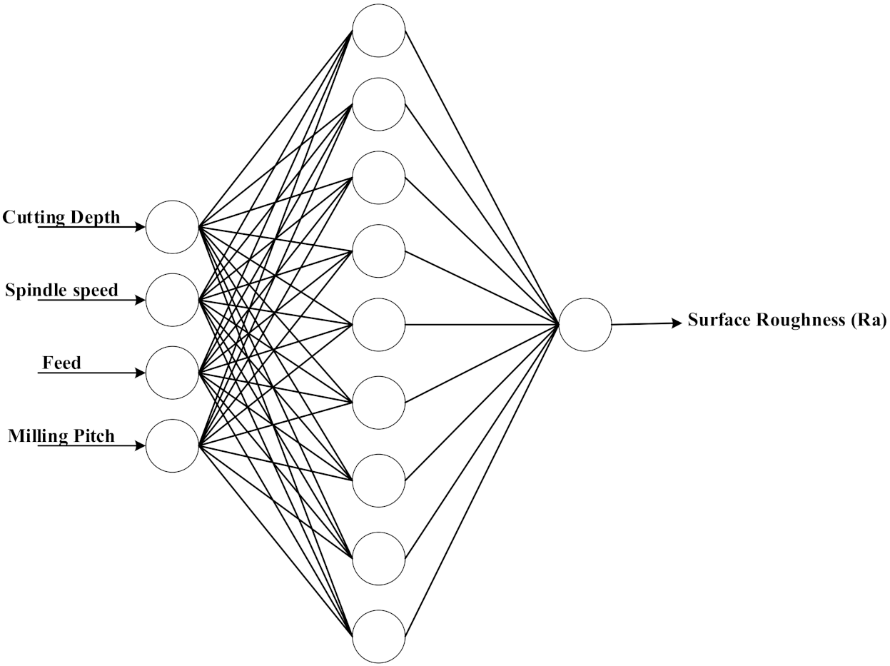
In this study, a three-layer BPNN was proposed (Figure 7). The input layer had four neurons, including the feed, spindle speed, cutting depth, and milling spacing. According to the experiment, the hidden layer was divided into 20 and 30 neurons. The following experiment was conducted to analyze the number of hidden layer neurons. One neuron in the output layer was surface roughness.

The target value of each training data back propagation neural network (T_n) and back propagation neural network output prediction (Y_n), calculation error, and RMSE were calculated between two calculations.

The RMSE is the square root of MSE and denotes the accuracy of the prediction and the degree of deviation between the predicted and target values. The smaller the value is, the higher the accuracy is.

The RMSE is calculated as follows:

$$\mathrm{RMSE}=\sqrt{\frac{1}{N}{\displaystyle \sum }_n^N{( T_n-Y_n)}^2}$$

(13)

where N is the total number of data.

We analyzed these parameters in

Table 11. Parameters of the back propagation neural network.

$\mathrm{Iteration} \left(\mathit{g}\right)$	500,000	1,000,000	2,000,000
$\mathrm{Learning} \mathrm{rate} \left(\mathit{\eta }\right)$	0.1	0.5	0.8
$\mathrm{Inertia} \mathrm{factor} \left(\mathit{\alpha }\right)$	0.5	0.8
$\mathrm{Number} \mathrm{of} \mathrm{hidden} \mathrm{layer} \mathrm{neurons} ( {\mathit{H}}_{\mathit{n}})$	20	30

. The iteration of the RMSE (g), vector (η, eta), inertial factor (α, alpha), and the number of hidden layer neurons (H_n) are depicted, and the RMSE values are listed in in Table 11.

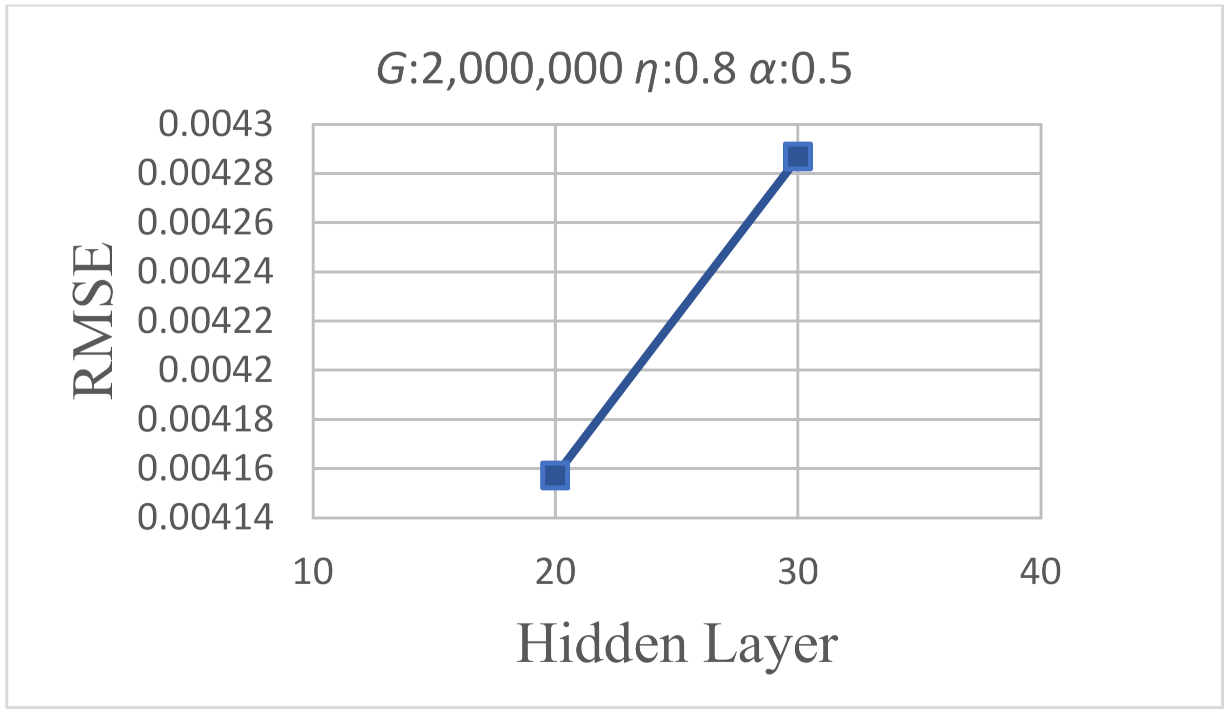
Too few neurons in the hidden layer can lead to large errors. Here, the number of hidden layer neurons was too large. Although the error value can be reduced, this slows the convergence rate.

Table 12. BPNN parameter experiment results.

No.	$\mathit{g}$	$\mathit{\eta }$	$\mathit{\alpha }$	${\mathit{H}}_{\mathit{n}}$	RMSE
1	500,000	0.1	0.5	20	0.006509797
2	500,000	0.1	0.5	30	0.006452063
3	500,000	0.1	0.8	20	0.006119852
4	500,000	0.1	0.8	30	0.006391917
5	500,000	0.5	0.5	20	0.005824562
6	500,000	0.5	0.5	30	0.005207749
7	500,000	0.5	0.8	20	0.005122899
8	500,000	0.5	0.8	30	0.005292113
9	500,000	0.8	0.5	20	0.005538547
10	500,000	0.8	0.5	30	0.005474869
11	500,000	0.8	0.8	20	0.005046593
12	500,000	0.8	0.8	30	0.00503299
13	1,000,000	0.1	0.5	20	0.006459028
14	1,000,000	0.1	0.5	30	0.006260511
15	1,000,000	0.1	0.8	20	0.00545881
16	1,000,000	0.1	0.8	30	0.005549763
17	1,000,000	0.5	0.5	20	0.005418789
18	1,000,000	0.5	0.5	30	0.005435733
19	1,000,000	0.5	0.8	20	0.004799067
20	1,000,000	0.5	0.8	30	0.004720272
21	1,000,000	0.8	0.5	20	0.005104896
22	1,000,000	0.8	0.5	30	0.005057594
23	1,000,000	0.8	0.8	20	0.004475259
24	1,000,000	0.8	0.8	30	0.004706842
25	2,000,000	0.1	0.5	20	0.005654144
26	2,000,000	0.1	0.5	30	0.005682413
27	2,000,000	0.1	0.8	20	0.005117443
28	2,000,000	0.1	0.8	30	0.005167562
29	2,000,000	0.5	0.5	20	0.004917882
30	2,000,000	0.5	0.5	30	0.004883775
31	2,000,000	0.5	0.8	20	0.00446712
32	2,000,000	0.5	0.8	30	0.004655432
33	2,000,000	0.8	0.5	20	0.004157405
34	2,000,000	0.8	0.5	30	0.004286702
35	2,000,000	0.8	0.8	20	0.00504091
36	2,000,000	0.8	0.8	30	0.00500624

indicates that the lowest RMSE was obtained for experiment 36. The inertia factor for all the experiments was 0.8. Next, we analyzed the RMSE changes for the four parameters (Figure 8, Figure 9, Figure 10 and Figure 11).

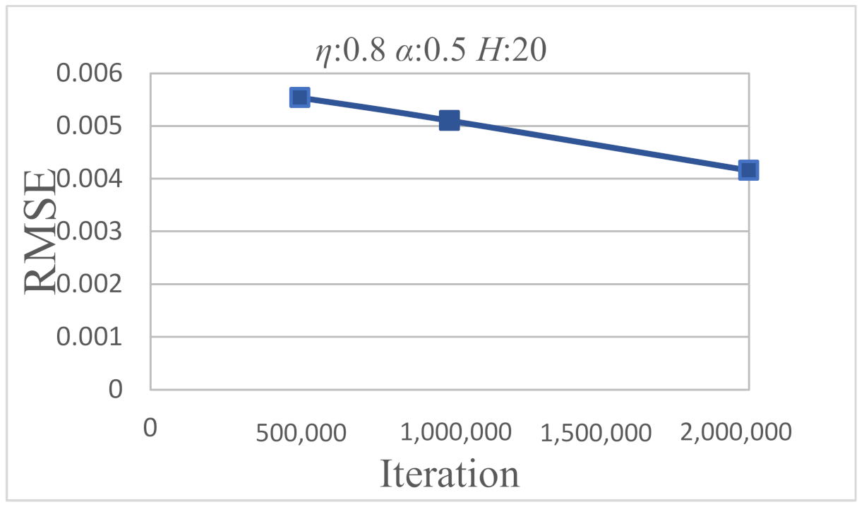
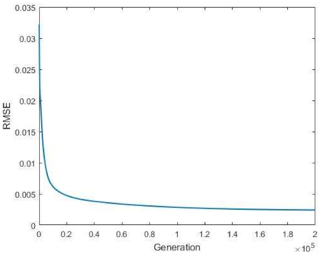
The results of the experiments indicated that the number of iterations increased from 500,000 to 1,000,000 and then to 2,000,000. The RMSE decreased with the increase in the number of iterations. However, iterations did not affect the training time, learning rate, and inertia factor.

According to Figure 10, the higher the learning rate is, the lower RMSE is.

The experiment result indicated that an increase in the inertia factor reduces the RMSE. If the value is too small, the error does not converge, resulting in the RMSE being too large.

The results in Figure 11 indicate that number of neurons in the hidden layer has a negligible effect on the RMSE. Too many neurons can result in divergence and can increase the training time, leading to increased errors.

3.4. Predictive Results of BPNN

According to Table 12, the lowest RMSE was obtained for experiment 36. Figure 12 illustrates the learning rate curve of each experiment and presents a representation of the convergence process and MSE. The learning rate graph was obtained by calculating the average value of 10 experiments.

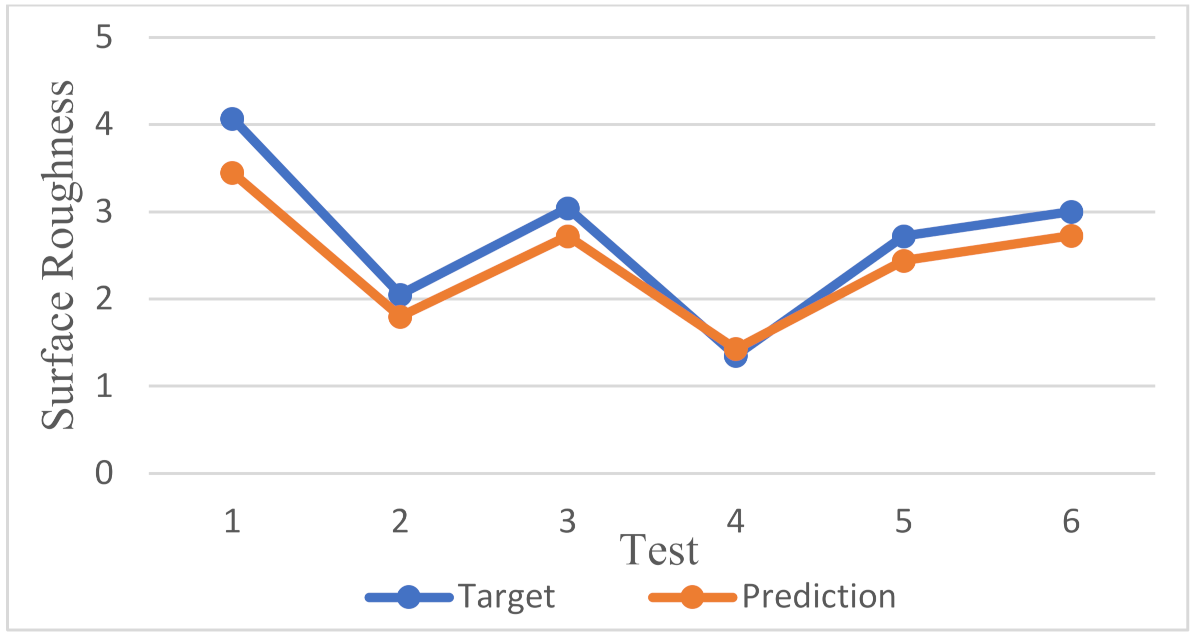
The measured value of the surface roughness instrument used in this experiment is the third place after the decimal point, and thus, the error value is required to be as small as possible. The changes in the target and predicted values listed are shown in Figure 13.

The coefficient ($R^2$) is used to measure the dependent variable and independent variables in statistical differences and explains the relationship between the target and predicted values. Typically, the value is between 0 and 1, and the value is closer to 1, which indicates excellent predictive power.

The determination coefficient is as follows:

$$R^2=1-\frac{S{S}_{res}}{S{S}_{tot}}=1-\frac{\sum {(T_n-Y_n)}^2}{\sum {(T_n-T)}^2}$$

(14)

where $S{S}_{res}$ is the sum of the residual square target and predicted values. $S{S}_{tot}$ is the sum of the target and average error. $Y_n$ is the predicted value, $T_n$ is the target value, and T is the target of the average.

The predication performance of linear regression was compared with that of BPNN. We substituted an input parameter into the equation to obtain the linear regression equation of surface roughness, which is expressed as follows:

$$Y=0.203+0.273x_1-0.357x_2+0.208x_3+0.022x_4$$

(15)

where Y is the surface roughness, $x_1$ is cutting depth, $x_2$ is spindle speed, $x_3$ is feed rate, $x_4$ is milling pitch

Table 13. BPNN parameter experiment results.

Model	RMSE	${\mathit{R}}^2$
Linear regression	0.021215796	0.7794
BPNN	0.008338854	0.9995

indicates that the RMSE of the BPNN was less than that of linear regression and that the $R^2$ value reached 0.9995, which is higher than that (0.7794) of linear regression, indicating that the BPNN is more accurate than linear regression.

4. Conclusions

In this study a BPNN was used to predict the surface roughness in CNC end milling. Furthermore, this study analyzed the influence of CNC parameters including cutting depth, spindle speed, feed rate, and milling pitch on surface roughness. The contributions of this study are summarized from the experimental results as follows.

(1)

In the measurement experiment of surface roughness, the CNC parameters with a smaller cutting depth, a faster spindle speed, and a smaller feed rate will obtain a better surface roughness.

(2)

According to ANOVA, the contributions of the cutting depth, spindle speed, feed rate, and milling pitch in CNC were 51.86%, 77.48%, 92.3%, and 71%, respectively. This result shows that the feed rate has a greater influence on the surface roughness.

(3)

In the process of training neural networks, when the used BPNN with the number of iterations is set to 2,000,000, the learning rate is set to 0.8, the inertia factor is set to 0.5, and the number of hidden layer neurons is set to 20 it will have a lower RMSE.

(4)

In this study, linear regression and the used BPNN were compared. From the experimental results, it can be verified that the used BPNN has a lower RMSE and a higher $R^2$. Furthermore, the prediction accuracy of linear regression and the used BPNN were 97.88% and 99.17%, respectively. According to the results, the used BPNN achieves excellent prediction of surface roughness.

References

1. Kohli, A.; Dixit, U.S. A neural-network-based methodology for the prediction of surface roughness in a turning process. Int. J. Adv. Manuf. Technol. 2004, 25, 118–129. [Google Scholar] [CrossRef]
2. Unune, D.R.; Mali, H.S. Artificial neural network–based and response surface methodology–based predictive models for material removal rate and surface roughness during electro-discharge diamond grinding of Inconel 718. Proc. Inst. Mech. Eng. Part B J. Eng. Manuf. 2016, 230, 2082–2091. [Google Scholar] [CrossRef]
3. Sharma, V.S.; Dhiman, S.; Sehgal, R.; Sharma, S.K. Estimation of cutting forces and surface roughness for hard turning using neural networks. J. Intell. Manuf. 2008, 19, 473–483. [Google Scholar] [CrossRef]
4. Tsao, C.C.; Hocheng, H. Evaluation of thrust force and surface roughness in drilling composite material using Taguchi analysis and neural network. J. Mater. Process. Technol. 2008, 203, 342–348. [Google Scholar] [CrossRef]
5. Sanjay, C.; Jyothi, C. A study of surface roughness in drilling using mathematical analysis and neural networks. Int. J. Adv. Manuf. Technol. 2006, 29, 846–852. [Google Scholar] [CrossRef]
6. Alagarsamy, S.V.; Ravichandran, M.; Meignanamoorthy, M.; Sakthivelu, S.; Dineshkumar, S. Prediction of surface roughness and tool wear in milling process on brass (C26130) alloy by Taguchi technique. Mater. Today Proc. 2020, 21, 189–193. [Google Scholar] [CrossRef]
7. Benardos, P.G.; Vosniakos, G.C. Prediction of surface roughness in CNC face milling using neural networks and Taguchi’s design of experiments. Robot. Comput. Integr. Manuf. 2002, 18, 343–354. [Google Scholar] [CrossRef]
8. Paturi, U.M.R.; Devarasetti, H.; Narala, S.K.R. Application of Regression and Artificial Neural Network Analysis In Modelling Of Surface Roughness In Hard Turning Of AISI 52100 Steel. Mater. Today Proc. 2018, 5, 4766–4777. [Google Scholar] [CrossRef]
9. Markopoulos, A.P.; Manolakos, D.E.; Vaxevanidis, N.M. Artificial neural network models for the prediction of surface roughness in electrical discharge machining. J. Intell. Manuf. 2008, 19, 283–292. [Google Scholar] [CrossRef]
10. Fredj, N.B.; Amamou, R. Ground surface roughness prediction based upon experimental design and neural network models. Int. J. Adv. Manuf. Technol. 2006, 31, 24–36. [Google Scholar] [CrossRef]
11. Bagci, E.; Işık, B. Investigation of surface roughness in turning unidirectional GFRP composites by using RS methodology and ANN. Int. J. Adv. Manuf. Technol. 2006, 31, 10–17. [Google Scholar] [CrossRef]
12. Ahmad, N.; Janahiraman, T.V.; Tarlochan, F. Modeling of Surface Roughness in Turning Operation Using Extreme Learning Machine. Arab. J. Sci. Eng. 2015, 40, 595–602. [Google Scholar] [CrossRef]
13. Ezugwu, E.O.; Fadare, D.A.; Bonney, J.R.; Silva, B.D.; Sales, W.F. Modelling the correlation between cutting and process parameters in high-speed machining of Inconel 718 alloy using an artificial neural network. Int. J. Mach. Tools Manuf. 2005, 45, 1375–1385. [Google Scholar] [CrossRef]
14. Karpat, Y.; Özel, T. Multi-objective optimization for turning processes using neural network modeling and dynamic-neighborhood particle swarm optimization. Int. J. Adv. Manuf. Technol. 2006, 35, 234–247. [Google Scholar] [CrossRef]
15. Lee, S.S.; Chen, J.C. On-line surface roughness recognition system using artificial neural networks system in turning operations. Int. J. Adv. Manuf. Technol. 2003, 22, 498–509. [Google Scholar] [CrossRef]
16. Karayel, D. Prediction and control of surface roughness in CNC lathe using artificial neural network. J. Mater. Processing Technol. 2009, 209, 3125–3137. [Google Scholar] [CrossRef]
17. Mulay, A.; Ben, B.S.; Ismail, S.; Kocanda, A. Prediction of average surface roughness and formability in single point incremental forming using artificial neural network. Arch. Civ. Mech. Eng. 2019, 19, 1135–1149. [Google Scholar] [CrossRef]
18. Zhong, Z.W.; Khoo, L.P.; Han, S.T. Prediction of surface roughness of turned surfaces using neural networks. Int. J. Adv. Manuf. Technol. 2005, 28, 688–693. [Google Scholar] [CrossRef]
19. Dhokia, V.G.; Kumar, S.; Vichare, P.; Newman, S.T.; Allen, R.D. Surface roughness prediction model for CNC machining of polypropylene. Proc. Inst. Mech. Eng. Part B J. Eng. Manuf. 2008, 222, 137–157. [Google Scholar] [CrossRef]
20. Sonar, D.K.; Dixit, U.S.; Ojha, D.K. The application of a radial basis function neural network for predicting the surface roughness in a turning process. Int. J. Adv. Manuf. Technol. 2005, 27, 661–666. [Google Scholar] [CrossRef]
21. Zerti, A.; Yallese, M.A.; Zerti, O.; Nouioua, M.; Khettabi, R. Prediction of Mechanical Engineers. Part C J. Mech. Eng. Sci. 2019, 233, 4439–4462. [Google Scholar] [CrossRef]
22. Thangarasu, S.S.; Mohanraj, T.; Devendran, K. Tool wear prediction in hard turning of EN8 steel using cutting force and surface roughness with artificial neural network. Proc. Inst. Mech. Eng. Part C J. Mech. Eng. Sci. 2019, 234, 329–342. [Google Scholar]
Figure 1. Surface roughness waveform.
Applsci 12 00393 g001
Figure 2. The arithmetic mean height of the contour curve.
Applsci 12 00393 g002
Figure 3. The influence of cutting depth on surface roughness.
Applsci 12 00393 g003
Figure 4. The influence of spindle speed on surface roughness.
Applsci 12 00393 g004
Figure 5. The influence of feed on surface roughness.
Applsci 12 00393 g005
Figure 6. The influence of milling pitch on surface roughness.
Applsci 12 00393 g006
Figure 7. Proposed BPNN architecture.
Applsci 12 00393 g007
Figure 8. Iteration variables for RMSE.
Applsci 12 00393 g008
Figure 9. Learning rate variables for RMSE.
Applsci 12 00393 g009
Figure 10. Inertia factor variables for RMSE.
Applsci 12 00393 g010
Figure 11. Number of hidden layer neuron variables for RMSE.
Applsci 12 00393 g011
Figure 12. Learning rate curves ( g : 2,000,000, η : 0.8, α : 0.5,   H n : 20).
Applsci 12 00393 g012
Figure 13. Target and predicted results of BPNN.
Applsci 12 00393 g013