Image Preprocessing Method in Radiographic Inspection for Automatic Detection of Ship Welding Defects

Abstract

Welding defects must be inspected to verify that the welds meet the requirements of ship welded joints, and in welding defect inspection, among nondestructive inspections, radiographic inspection is widely applied during the production process. To perform nondestructive inspection, the completed weldment must be transported to the nondestructive inspection station, which is expensive; consequently, automation of welding defect detection is required. Recently, at several processing sites of companies, continuous attempts are being made to combine deep learning to detect defects more accurately. Preprocessing for welding defects in radiographic inspection images should be prioritized to automatically detect welding defects using deep learning during radiographic nondestructive inspection. In this study, by analyzing the pixel values, we developed an image preprocessing method that can integrate the defect features. After maximizing the contrast between the defect and background in radiographic through CLAHE (contrast-limited adaptive histogram equalization), denoising (noise removal), thresholding (threshold processing), and concatenation were sequentially performed. The improvement in detection performance due to preprocessing was verified by comparing the results of the application of the algorithm on raw images, typical preprocessed images, and preprocessed images. The mAP for the training data and test data was 84.9% and 51.2% for the preprocessed image learning model, whereas 82.0% and 43.5% for the typical preprocessed image learning model and 78.0%, 40.8% for the raw image learning model. Object detection algorithm technology is developed every year, and the mAP is improving by approximately 3% to 10%. This study achieved a comparable performance improvement by only preprocessing with data.

1. Introduction

Welding defects must be inspected to verify that the welds meet the requirements of ship welded joints in order for them to support their own weight and the cargo weight during the lifetime of ships and perform their role without breakage by having resistance to stress, corrosion, and fatigue cracking. Destructive and nondestructive inspection methods have been applied to welding joints. Destructive inspections have high reliability; however, performing them directly on welding joints is unreasonable. Further, performing destructive inspections on all joints is difficult. Nondestructive inspections are widely applied during the production process because they can determine pass or fail based on quality standards, by measuring and detecting physical properties that change because of defects without damaging the weld zone. To perform nondestructive inspections, the completed weldment must be transported to the nondestructive inspection station or the inspection equipment must be installed on site; however, this process is expensive. Therefore, methods to instantly inspect welding defects on site, while taking into consideration the locations that are difficult for field workers to access, are necessary [1].

Thus, the automation of welding defect detection is required. Recently, machine vision [2] technology has been developed because the use of vision-based defect detectors using cameras has become universalized. Accordingly, artificial intelligence has been employed for defect detection using image processing, and at several processing sites of companies, continuous attempts are being made to combine machine vision and deep learning [3] to detect defects more accurately [4]. The data preprocessing step performed before training a deep learning model involves changing the existing data to data suitable for the learning algorithm. Such a preprocessing step is also applied to new data to be predicted after the model is created, and the more the deep learning algorithm goes through the preprocessing step, the better the learning performance [5]. Therefore, in the study of creating a welding defect detection algorithm using deep learning, the preprocessing of welding defects in radiographic images before algorithm creation has a great effect on improving the accuracy of the welding defect detection algorithm [6,7]. However, the data preprocessing step has not been consistent, and a technique optimized for welding defects has not been proposed. In general, Contrast Limited Adaptive Histogram Equalization (CLAHE) and image denoising are used in the preprocessing step for generating a radiographic detection algorithm [8,9].

This study aimed to express the welding defect part more conspicuously than in the raw image. The preprocessing algorithm using CLAHE, image denoising, thresholding, and concatenation was applied to analyze the defect characteristics according to the purpose and reflect the defect characteristics. Then, the mean average precision (mAP) was checked by comparing the typical preprocessing, the non-preprocessing, and the preprocessing algorithm we proposed.

2. Preprocessing Method

In general, types of image preprocessing applied in deep learning include denoising, cropping, thresholding, binarization, morphology transformation, and more. The goal of image preprocessing method for welding defect is to change the intensity difference between the background part and the defect part to a certain level or more, and to change the characteristics of the defined black defect and white defect to appear. According to the above purpose, image preprocessing was performed by applying histogram equalization, denoising, and thresholding. After that, in order to reflect the characteristics of white and black defects, concatenation was performed to compose three channels of the raw image, the thresholded image expressing the characteristics of the black defect and the thresholded images expressing the characteristics of the white defect.

2.1. Histogram Equalization

Histogram equalization (HE) is used to obtain contrast-enhanced images by generating a mapping function using the histogram probability distribution of the input images and the cumulative distribution generated on this basis. HE can be performed appropriately only if the distribution of the pixel intensity is identical over the entire image by performing the redistribution of pixel intensity using one histogram. If a part of the image has a different distribution from the other regions, the image to which HE is applied would be distorted.

In contrast to HE, which can be applied only if the distribution of pixel intensity is identical in the entire image, adaptive histogram equalization (AHE) [10] divides an image into multiple parts using a grid and applies HE to each sub-image. Therefore, this method is suitable for adjusting the local contrast of an image because the image contrast within a given grid is improved. However, AHE has the disadvantage of generating a large peak (that is, an amplified noise), even if there is a noise that shows an extremely small difference from the other regions when the pixel intensities in a random grid are concentrated in an extremely small region because the pixel intensities in that region are spread to a large region.

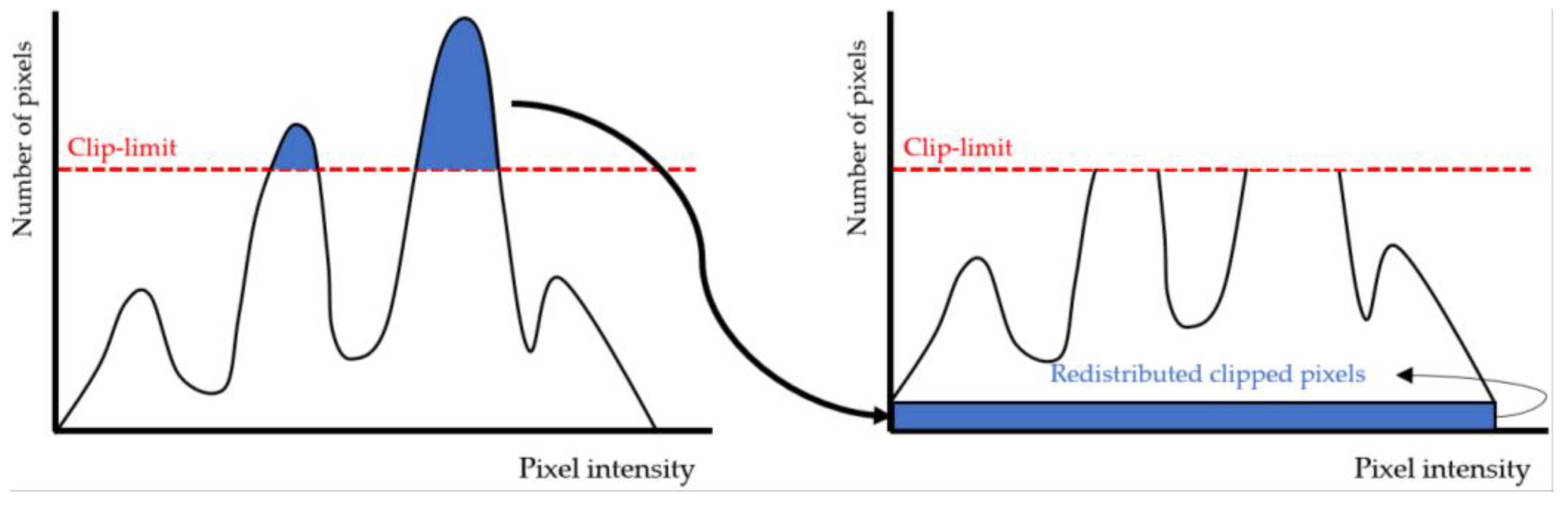
CLAHE is a variant of AHE that applies limitations to contrast to solve the noise amplification problem of AHE [11]. It redistributes pixels above a specific height by applying a limitation to the histogram height before calculating the cumulative distribution function (CDF), as shown in Figure 1. In this process, it limits the gradient of the CDF such that it does not become too high. Finally, the CLAHE-applied image is obtained by applying HE to the CDF [12]. 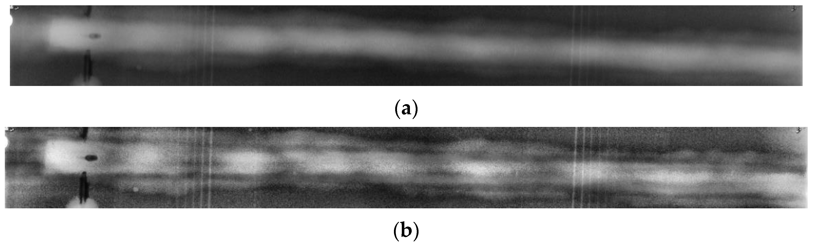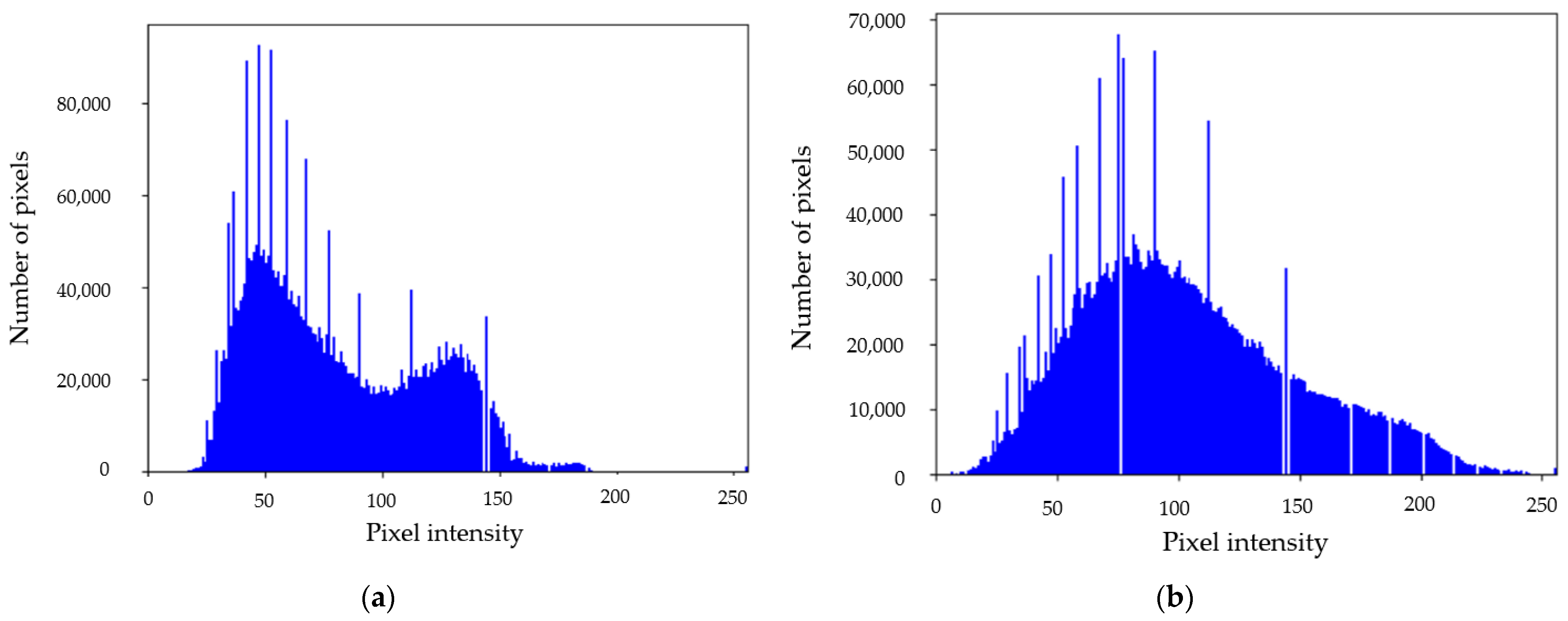Figure 2 shows a higher contrast through the raw image and the CLAHE-applied image, and the histogram of each image shows how the pixel values are spread by applying CLAHE, as shown in Figure 3.

2.2. Denoising

After CLAHE is applied to images, noise that degrades data quality increases [13]. Because noise lowers the performance and accuracy of the algorithm, denoising is performed for CLAHE-applied images.

The nonlocal means (NLM) algorithm [14] reduces noise by performing a weighted average of pixel values. Images are defined over a discrete regular grid $\mathsf{\Omega }$ of dimension $d$ and cardinality $\left|\mathsf{\Omega }\right|$. $v$ denotes the original image, the value of the restored image $u$ at a site $s\in \mathsf{\Omega }$ is defined as the convex combination

$$u\left(s\right)=\frac{1}{Z\left(s\right)}{\displaystyle \sum }_{t\in \mathcal{N}\left(s\right)}w\left(s, t\right)v\left(t\right)$$

(1)

where $w\left( , \right)$ are non-negative weights, Z(s) is a normalization constant such that for any site s we have $Z\left(s\right)={\displaystyle \sum }_{t\in \mathcal{N}\left(s\right)}w\left(s, t\right)$, and $\mathcal{N}\left(s\right)$ corresponds to a set of neighboring sites of $s$. $w\left(s, t\right)$ is the weight for each region, at sites $s$ and $t$. The weight for each region can be expressed as follows [14,15]:

$$w\left(s, t\right)=g_h\left({\displaystyle \sum }_{\delta \in ∆}{G}_{\sigma }\left(\delta \right){\left(v\left(s+\delta \right)-v\left(t+\delta \right)\right)}^2\right)$$

(2)

In Equation (2), $G_{\sigma }$ represents a Gaussian distribution in the ${\sigma }^2$ size, $g_h:{ℝ}^{+}\to {ℝ}^{+}$ is a continuous non-increasing function with $g_h\left(x\right)=e^{-\frac{x^2}{h^2}}$, and $∆$ represents the discrete patch region containing the neighboring sites $\delta$. $h$ is used to control the amount of filtering. Thus, NLM algorithm restores an image by performing a weighted average of pixel values taking into account spatial and intensity similarities between pixels.

The NLM algorithm is highly effective for denoising but takes a considerable amount of time because it involves several calculations. Hence, several researchers have attempted to reduce the time taken by this algorithm through acceleration using a GPU and improving the algorithm. Therefore, the process of calculating the weight $w\left(s, t\right)$, which requires a considerable amount of time in the NLM algorithm, was changed from 2D to 1D, and the calculation was performed with a precalculated value. Given a translation vector $d_x$, a new image $S_{d_x}$ can be expressed as follows [15]:

$$S_{d_x}\left(p\right)={\displaystyle \sum }_{k=0}^p{\left(v\left(k\right)-v\left(k+d_x\right)\right)}^2, p\in \mathsf{\Omega }$$

(3)

$S_{d_x}$ corresponds to the discrete integration of the squared difference of the image $v$ and its translation by $d_x$. Under 1D assumption $\mathsf{\Omega }$ is $\mathsf{\Omega }=⟦0, n-1⟧$, an image with $n$ pixels. In 1D, patches of the form $∆=⟦-P, P⟧$ are used to compute the weight for two pixels $s$ and $t$. By replacing the Gaussian distribution by a constant without noticeable differences. Thus Equation (2) rewrites as follows [15]:

$$w\left(s, t\right)=g_h\left({\displaystyle \sum }_{{\delta }_x\in ∆}{\left(v\left(s+{\delta }_x\right)-v\left(t+{\delta }_x\right)\right)}^2\right)$$

(4)

Let $d_x=\left(t-s\right)$ and define $\widehat{p}=\left(s+{\delta }_x\right)$. With this reparametrization, $w\left(s, t\right)$ can be expressed as $w\left(s, t\right)=g_h({\displaystyle \sum }_{\widehat{p}=s-P}^{s+P}{\left(v\left(\widehat{p}\right)-v\left(\widehat{p}+d_x\right)\right)}^2)$. If split the sum and use the identity in Equation (3), $w\left(s, t\right)$ rewrites as shown in Equation (5) [15].

$$w\left(s, t\right)=g_h\left(S_{d_x}\left(s+P\right)-S_{d_x}\left(s-P\right)\right)$$

(5)

In the case of this calculation, the required amount of computation is determined independently of the patch size; this significantly reduces the algorithm computation time, thus facilitating efficient computation.

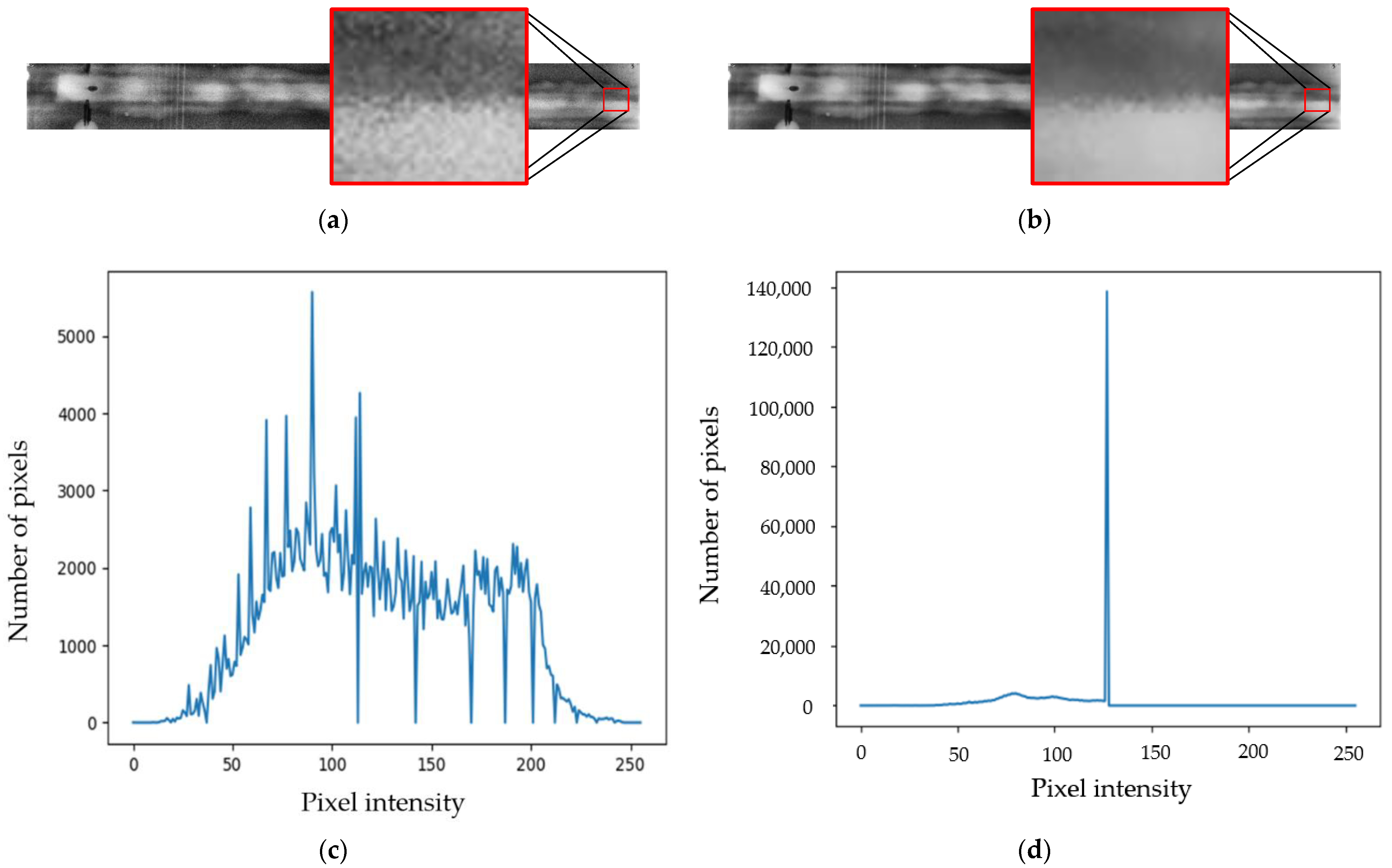
Figure 4 shows the partially enlarged image before denoising and after denoising, quality improvement of the image after denoising and histogram distribution of the enlarged image. The quality is improved and pixel intensities of the image are concentrated in one part after denoising.

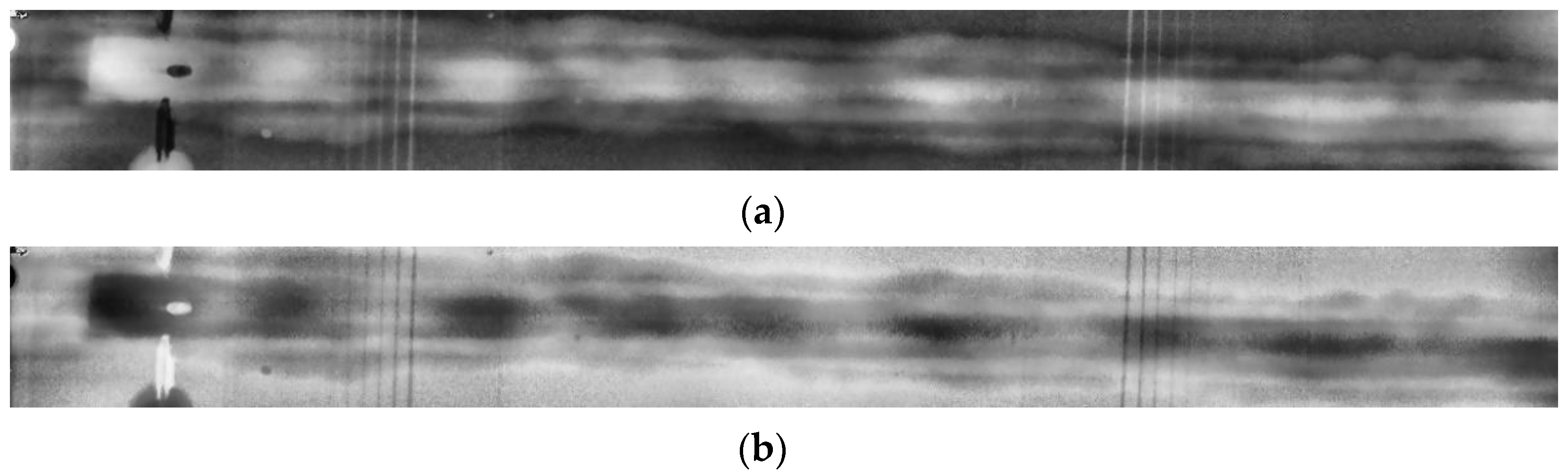
Defects, such as porosities and incomplete penetrations, which account for 90% of all welding defects, have low pixel values. Thus, the image was denoised, as shown in Figure 5a. For excessive penetrations and slag inclusions, which have higher pixel values than the background part, the image with reversed pixel values was also denoised, as shown in Figure 5b.

2.3. Thresholding

Training a deep learning model with data requires the normalization of the data to improve the learning efficiency by readjusting the input image or through normalization and to facilitate the use of an activation function that converts the total sum of input signals to output signals in deep learning [16]. The data were normalized to the range of [−1, 1] by removing the unnecessary parts of the background by analyzing the pixel values of the welding defect and background parts and setting the threshold at a pixel value of 127.5.

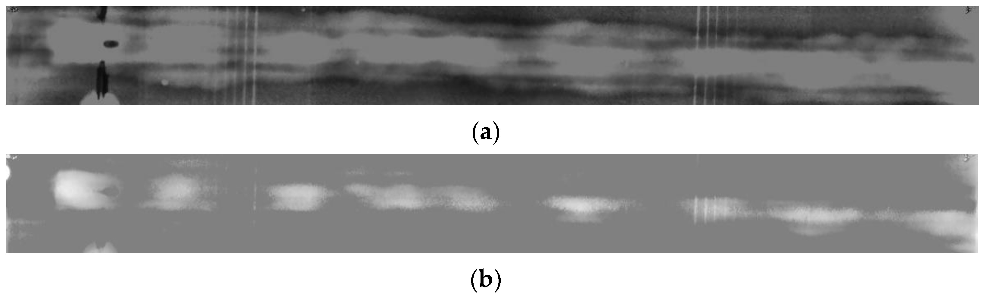
The defects that have a pixel value lower than the background part statistically have a value lower than 127.5, and the background part has a pixel value higher than 127.5. By setting the threshold to 127.5, the pixel values higher than the threshold were modified to 127.5, and the pixel values lower than the threshold were maintained, as shown in Figure 6a.

For the defects having a pixel value higher than the background part, the image in Figure 5b, wherein the pixel values were reversed in the denoising step, was used. In this image, the pixel values lower than the threshold were modified to 0, and the pixel values higher than the threshold were maintained and reversed again, as shown in Figure 6b.

2.4. Defect Thresholding Concatenate Image

In order to express the characteristics of the data to be expressed in one place, each new datum that has analyzed the characteristics of the data is expressed to form a layer through concatenation [17,18,19]. The welding defect data in this paper has two types of defects. One is a black defect with a lower pixel value than the background part, and the other is a white defect with a higher pixel value than the background part. It is necessary to express the characteristics of these two defects as one datum.

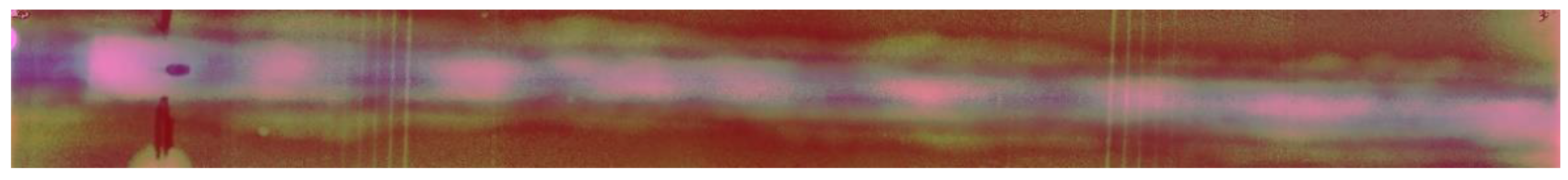
Input data was constructed through image concatenation to detect white and black defects in one algorithm, so that the characteristics of each image could be expressed in each algorithm. Thresholding that can contain black information as shown in Figure 6a is placed in channel 2, and thresholding that can contain white information as shown in Figure 6b is arranged in channel 3, and then combined to form one image. The final preprocessed image is constructed by two thresholded images and the raw image without CLAHE to grayscale so that the image pixel values are composed of three channels, as shown in Figure 7. Unlike when only the raw image is used, each additional information is included in channels 2 and 3, which improves performance. The process of preprocessing is shown in Algorithm 1.

Algorithm 1: Radiographic inspection image preprocessing

Input: Raw image, Threshold value: $v_T$, Max value: $v_M$ Output: Preprocessed image   For Raw image in images:        lab = convert color (Raw image, BGR to LAB)      l, a, b = split channel (lab)      clahe l = CLAHE (l)      Image = merge channel (clahe l, a, b)        Denoised image = Fast nonlocal means denoising (Image)      Denoised and reversed image = bitwise not (Denoised image)        Image = convert color (Denoised image, BGR to grayscale)      Reversed image = convert Color (Denoised and reversed image, BGR to grayscale)      Threshold = THRESHOLD (Image, $v_T$$, v_M$, THRESH_TRUNC)      Threshold reverse = THRESHOLD (Reversed image, $v_T$$, v_M$, THRESH_TRUNC)      Threshold reverse = bitwise not (Threshold reverse)        Preprocessing image = merge channel (Image, Threshold, Threshold reverse)

3. Experimental Method

3.1. Composition of Dataset

The training dataset was used to train the model. The validation dataset was used to determine how well the model was trained using the training dataset. A test dataset was used to evaluate the performance of the model. The training dataset, validation dataset, and test dataset were composed of 6:2:2 as shown in Figure 8.

As the welding defects consisted of a total of 320 data points, the training dataset was composed of 192 data points, and the validation and test datasets were composed of 64 data points each. When the radiographic inspection images themselves are used for learning, the learning rate is lowered due to noise such as the shooting date, image quality indicator (IQI) and weld seam number in the images. Therefore, only the bead part was cut from the radiographic inspection images and used for learning.

Among the defects present in the data, porosity and incomplete penetration with lower pixel values compared to beads, which are background parts, were labeled as black defects, and excessive penetration and slag inclusion with higher pixel values than beads were labeled as white defect. The 256 points of data used in training were of various sizes. High-quality images increase the number of parameters to be learned and lower the learning speed, as well as overload the computer during learning and cause learning to be stopped, so images were readjusted to 1280 × 1280 [20].

3.2. Object Detection Deep Learning Model

The You Only Look Once (YOLO) algorithm [21] was used to demonstrate the performance improvement in the object detection model of welding defect preprocessed images.

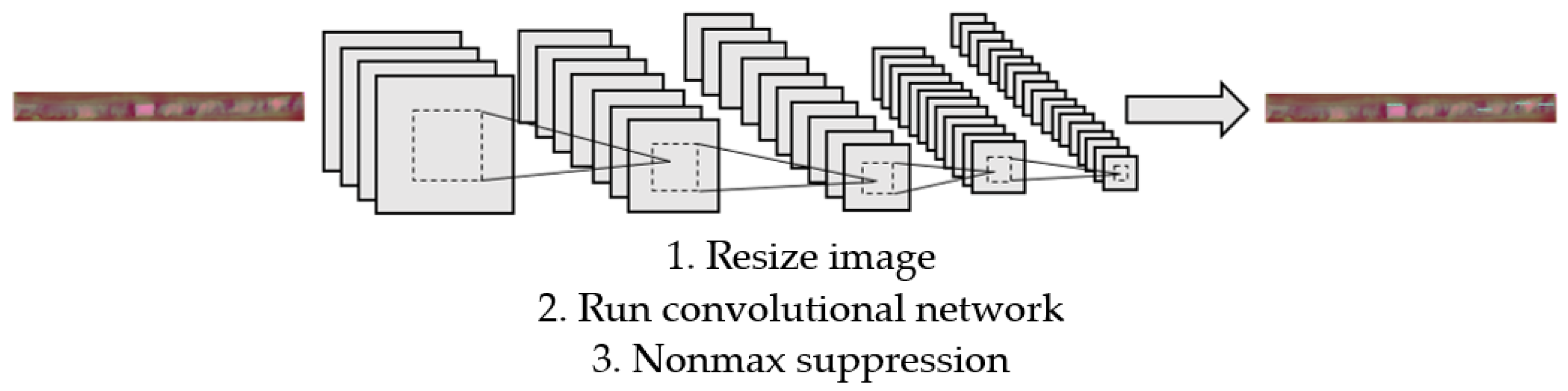
The structure of the YOLO algorithm based on a convolutional neural network (CNN) is shown in Figure 9. Object detection and recognition were integrated into one system after using the estimation method according to the unit configuration of the final output layer and the fixed segmentation for the input image in the existing method. Consequently, this algorithm can perform object detection more than 1000 times faster than the Region-based Convolutional Network method (R-CNN) and more than 100 times faster than Fast R-CNN (R-CNN and fast R-CNN are widely used deep learning-based object detection methods) [22].

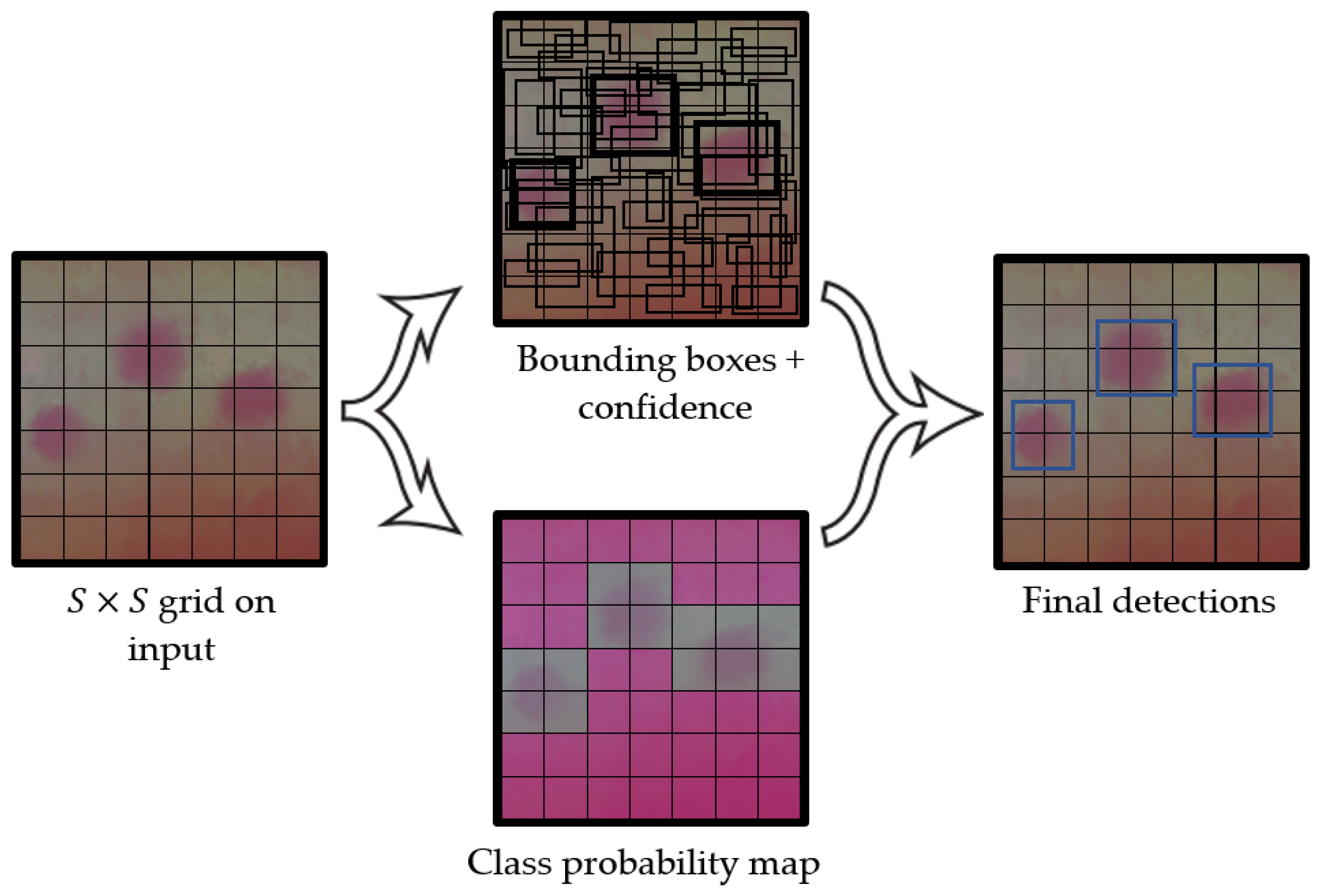
Figure 10 shows an overview of the YOLO model. The YOLO algorithm divides the input image into S × S square grid cells, which then are divided into squares based on the formed cells. Next, the probability that each square would include objects is calculated. Subsequently, the result of object detection using the YOLO algorithm is shown by outputting squares for the case where the threshold is exceeded based on the probability that the squares would include objects [21].

3.3. Generalized Intersection over Union (GIoU) Loss

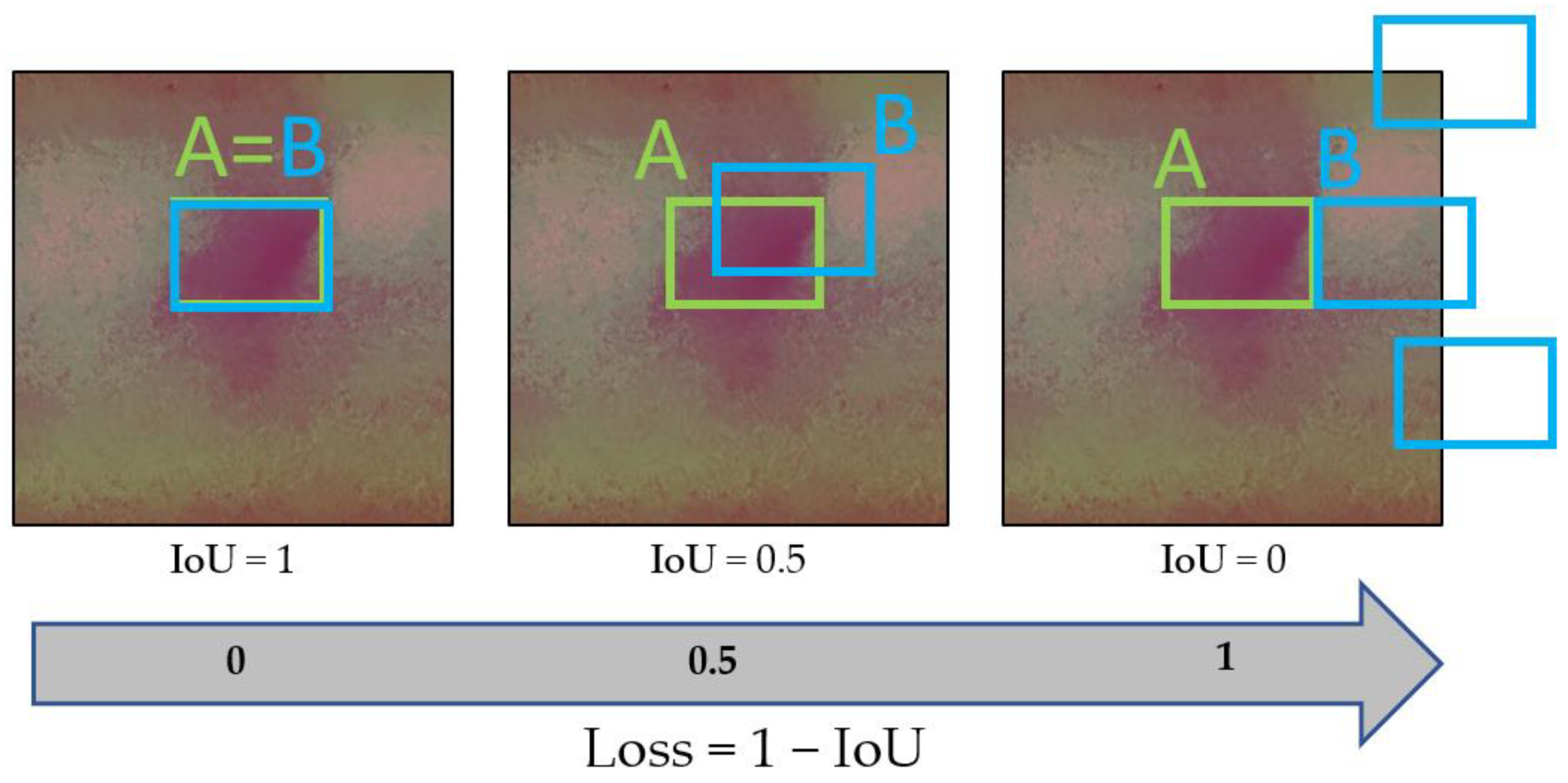
When the intersection over union (IoU) is used to formulate a loss function, 1 − IoU is used as an index so that the more overlapping there is between the ground truth boxes A and the prediction box B, the closer this value is to zero, as shown in Figure 11. In general, the loss must be closer to 0 if the prediction is better, and the loss must be higher if the prediction is worse. However, as shown in the last figure in Figure 11, the general IoU becomes 0 if there is no intersection between the two boxes. Thus, it is uncertain whether the intersection did not occur because the prediction is closer to the ground truth or because of a large error. The process of calculating the loss function using IoU is shown in Algorithm 2.

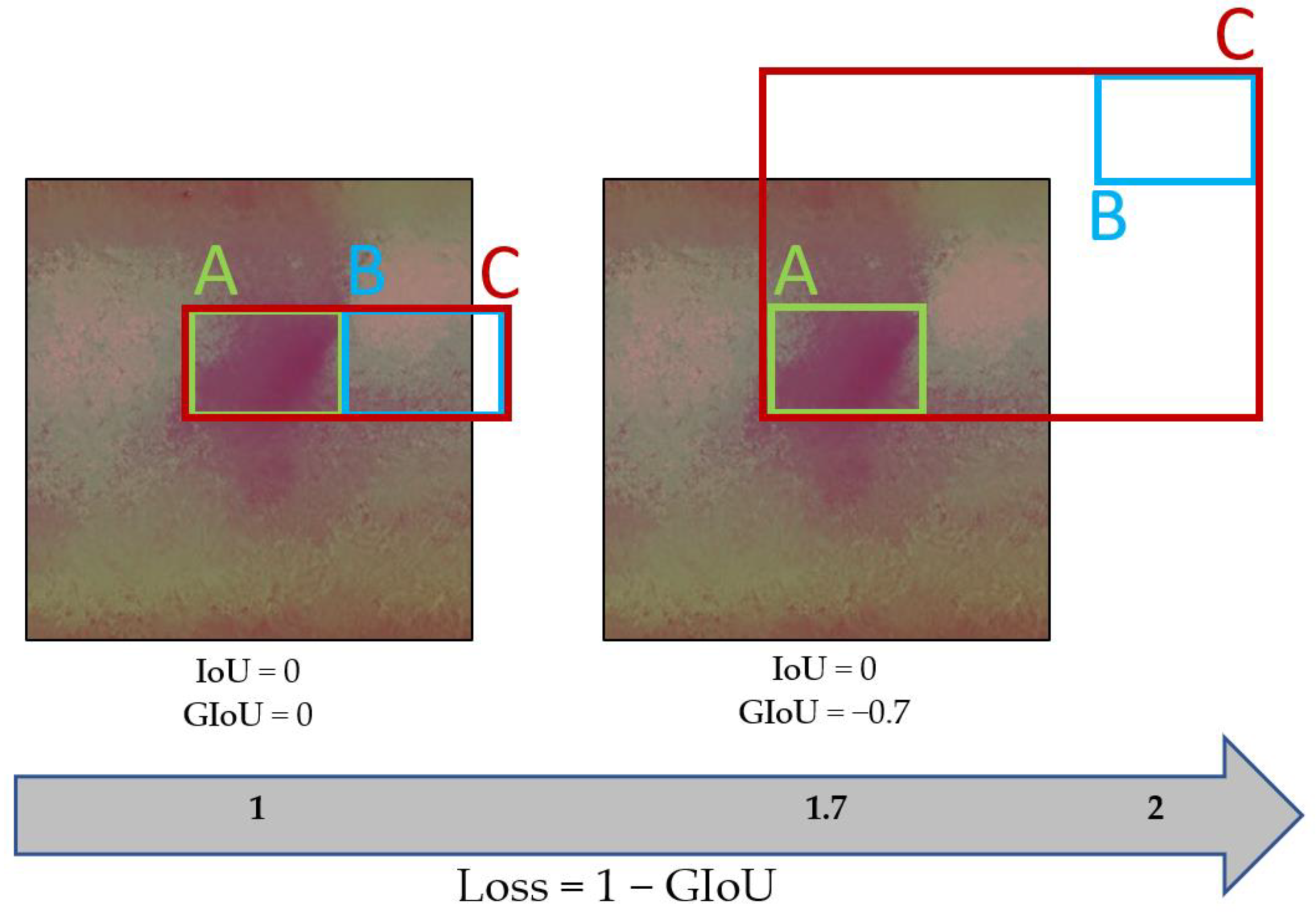
The afore mentioned problem is solved through a loss function using the generalized intersection over union (GIoU). In the GIoU, the smallest box C that covers the ground truth box and precision box in the IoU box is added, as shown in Figure 12. The GIoU is defined as follows:

$$\mathrm{GIoU}=\mathrm{IoU}-\frac{\left|\mathrm{C}-\left(\mathrm{A}{\displaystyle \cup }\mathrm{B}\right)\right|}{\left|\mathrm{C}\right|}$$

(6)

If the distance between boxes A and B becomes infinite, the GIoU converges to −1.

Thus, if there is no intersection between boxes A and B, the IoU is 0 in all cases, whereas the GIoU value changes depending on the distance between the two boxes; hence, whether the intersection is not generated because the prediction is close to the ground truth or because of a large error can be distinguished [23]. The process of calculating loss function using GIoU is shown in Algorithm 2.

Algorithm 2: IoU and GIoU as bounding box losses

$\mathrm{Input}: \mathrm{Predicted} B^p$$\mathrm{and} \mathrm{ground} \mathrm{truth} B^g \mathrm{bounding} \mathrm{box} \mathrm{coordinates}:$ $B^p=\left(x_1^p, y_1^p, x_2^p, y_1^p\right)$$, B^g=\left(x_1^g, y_1^g, x_2^g, y_1^g\right)$ $\mathrm{output}: L_{IoU}, L_{GIoU}$    1. $\mathrm{For} \mathrm{the} \mathrm{predicted} \mathrm{box} B^p$$, \mathrm{ensuring} x_2^p>x_1^p$$\mathrm{and} y_2^p>y_1^p:$ ${\widehat{x}}_1^p=min\left(x_1^p, x_2^p\right)$$, {\widehat{x}}_2^p=max\left(x_1^p, x_2^p\right)$$, {\widehat{y}}_1^p=min\left(y_1^p, y_2^p\right)$$, {\widehat{y}}_2^p=max\left(y_1^p, y_2^p\right)$    2. $\mathrm{Calculating} \mathrm{area} \mathrm{of} B^g :A^g=\left(x_2^g-x_1^g\right)\times \left(y_2^g-y_1^g\right)$    3. $\mathrm{Calculating} \mathrm{area} \mathrm{of} B^p :A^p=\left({\widehat{x}}_2^p-{\widehat{x}}_1^p\right)\times \left({\widehat{y}}_2^p-{\widehat{y}}_1^p\right)$    4. $\mathrm{Calculating} \mathrm{intersection} \mathrm{I} \mathrm{between} B^p$$\mathrm{and} B^g:$ $x_1^I=max\left({\widehat{x}}_1^p, x_1^g\right)$$, x_2^I=min\left({\widehat{x}}_2^p, x_2^g\right)$$, y_1^I=max\left({\widehat{y}}_1^p, y_1^g\right)$$, y_2^I=min\left({\widehat{y}}_2^p, y_2^g\right)$    5. $\mathrm{Finding} \mathrm{the} \mathrm{coordinate} \mathrm{of} \mathrm{smallest} \mathrm{enclosing} \mathrm{box} B^c:$ $x_1^c=min\left({\widehat{x}}_1^p, x_1^g\right)$$, x_2^c=max\left({\widehat{x}}_2^p, x_2^g\right)$$, y_1^c=min\left({\widehat{y}}_1^p, y_1^g\right)$$, y_2^c=max\left({\widehat{y}}_2^p, y_2^g\right)$    6. $\mathrm{Calculating} \mathrm{area} \mathrm{of} B^c$$: A^c=\left(x_2^{\mathrm{c}}-x_1^c\right)\times \left(y_2^c-y_1^c\right)$    7. $IoU=\frac{\mathrm{I}}{u},$$\mathrm{where} u=A^p+A^g-I$    8. $GIoU=IoU-\frac{A^c-u}{A^c}$    9. $L_{IoU}=1-IoU$$, L_{GIoU}=1-GIoU$

3.4. Mean Average Precision (mAP)

The mAP indicator uses recall and precision, which are used as performance indicators of binary classifiers, and it is used to evaluate the performance of an object detection algorithm.

Table 1. Confusion matrix.

		Predict
		Positive	Negative
Ground Truth	Positive	True Positive	False Negative
	Negative	False Positive	True Negative

depicts a comparison of the actual and predicted values to measure the performance of the trained model.

Precision is the ratio of correct detections among all the detection results and can be expressed as follows:

$$\mathrm{Precision}=\frac{\mathrm{TP}}{\mathrm{TP}+\mathrm{FP}}=\frac{\mathrm{TP}}{\mathrm{all} \mathrm{detections}}$$

(7)

Recall is the ratio of accurately detected objects among the objects to be detected, and it can be expressed as follows:

$$\mathrm{Recall}=\frac{\mathrm{TP}}{\mathrm{TP}+\mathrm{FN}}=\frac{\mathrm{TP}}{\mathrm{all} \mathrm{ground} \mathrm{truths}}$$

(8)

After the precision–recall (PR) curve [24] is obtained through the changes in precision and recall according to the change in the threshold by the confidence level, the average precision (AP), which has the area under the graph in the PR curve as its value, is determined. The AP is then averaged for each class to determine the mAP. To represent the performance of the algorithm, mAP, which is a PASCAL visual object class performance evaluation method, is used as a performance indicator for object detection [25].

4. Results

4.1. Preprocessing Results

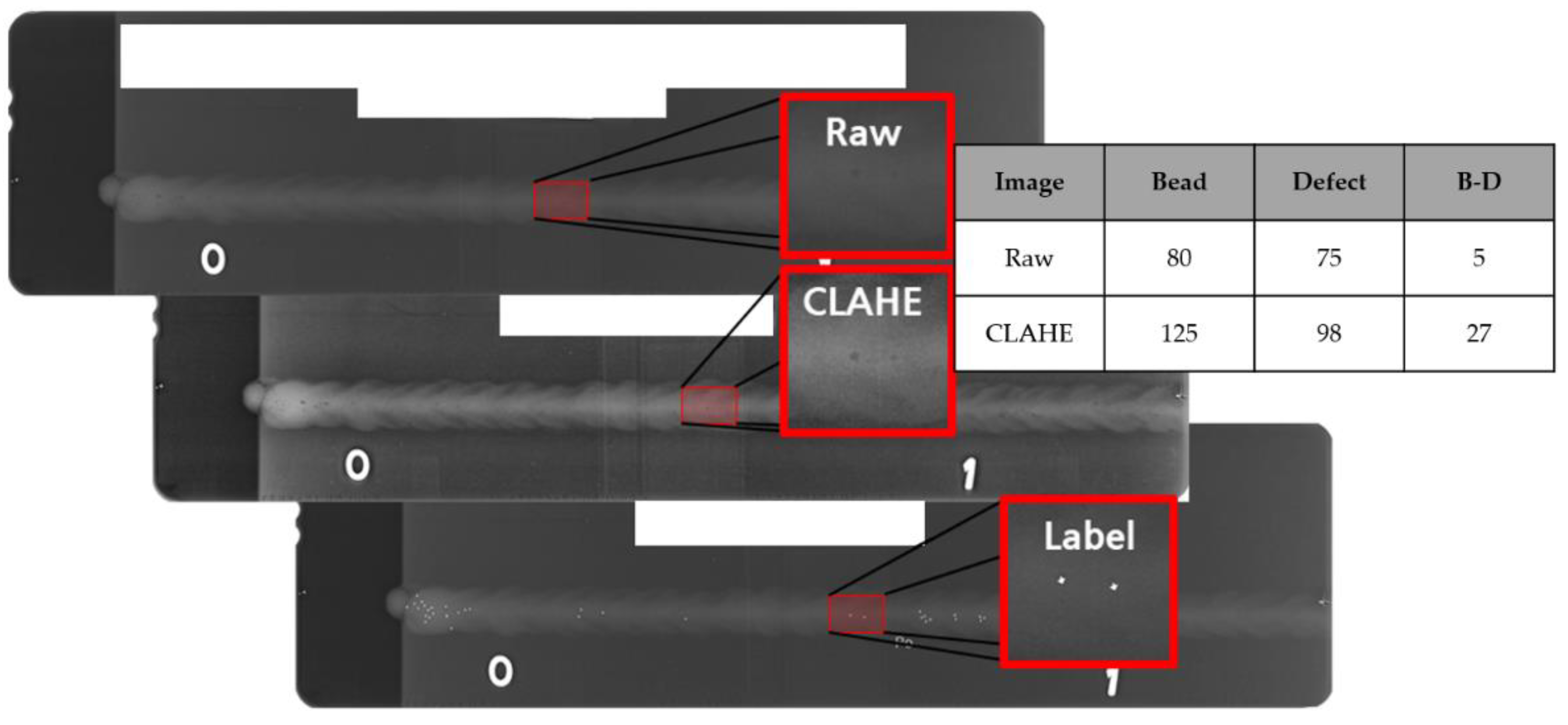
As shown in Figure 13, the degree of change because of CLAHE was measured by analyzing and measuring the pixels of the bead, which represent the background part and welding defect part. In the raw image, the pixel value of the bead, the background part, was 80, whereas the pixel value of the defect part was 75, showing a difference of 5. In the CLAHE-applied image, the pixel value of the bead was 125, whereas the pixel value of the defect part was 98, showing a difference of 27.

Table 2. Welding defect before applying CLAHE and after applying CLAHE.

		Lower Pixel Intensity than Background (Black Defect)			Higher Pixel Intensity than Background (White Defect)
	Level	1	2	3	1	2	3
	Pixel	30–	15–30	0–15	30–	15–30	0–15
Before applying CLAHE	Defect	83	131	883	20	34	66
After applying CLAHE	Defect	265	422	420	76	24	10

shows the results of the raw image before applying CLAHE and the image after applying CLAHE by improving the entire defect data. Object detection in computer vision is mainly performed using pattern recognition. The recall becomes low unless the difference between the object and the background part is above a certain level [26]. Therefore, the defects in the data were divided into three levels, and the objects were classified based on the difference in pixels between the object and the background part. Level 1 is a difference of 30 pixels or more between the bead and defect, Level 2 is a difference of 15–30, and Level 3 is a difference of 0–15. The higher the level, the more difficult it is to distinguish between the bead and defect. Consequently, among the defects with a pixel value lower than the background part, the number of Level 3 defects decreased from 883 to 420. Among the defects with a pixel value higher than the background part, the number of Level 3 defects decreased from 66 to 10.

4.2. Object Detection Result

In the case of the preprocessing method we proposed and the typical preprocessing method, the noise that hindered learning was removed after CLAHE was applied. The CNN model requires several computing resources if it is trained with the original pixel values of the image because each pixel has a value of 0–255. In the preprocessing method we proposed, after thresholding the raw images so that the pixels are normalized, the thresholded image, the reverse thresholded image, and raw image are merged into three channels to reflect the features of white and black defects.

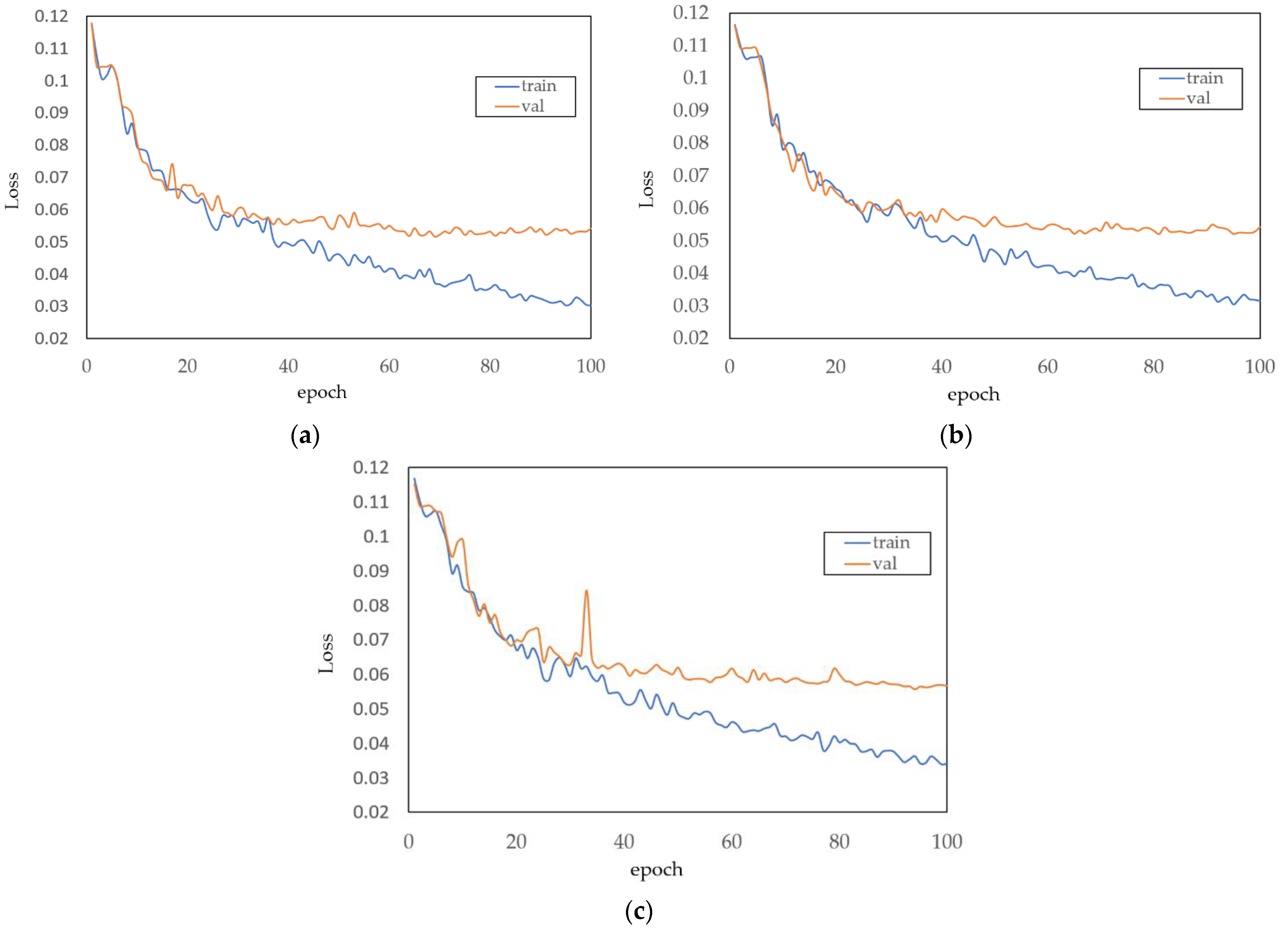
The loss graph and mAP for learning were derived by training the YOLO algorithm with the raw images, typical preprocessed images and preprocessed images of the welding defects. Figure 14 shows the loss graphs of the preprocessed, typical preprocessed and raw image learning models. The loss on the training dataset for the preprocessed image learning model, typical preprocessed image learning model, and the raw image learning model, converged to 0.03019, 0.031688 and 0.03415. The loss on the test dataset for the preprocessed image learning model, typical preprocessed image learning model, and the raw image learning model, converged to 0.05406, 0.05434 and 0.05674. In the loss graph of the three learning models, both the loss on the training data and the loss on the validation data show a decreasing trend, so it can be judged that overfitting did not occur in the trained models.

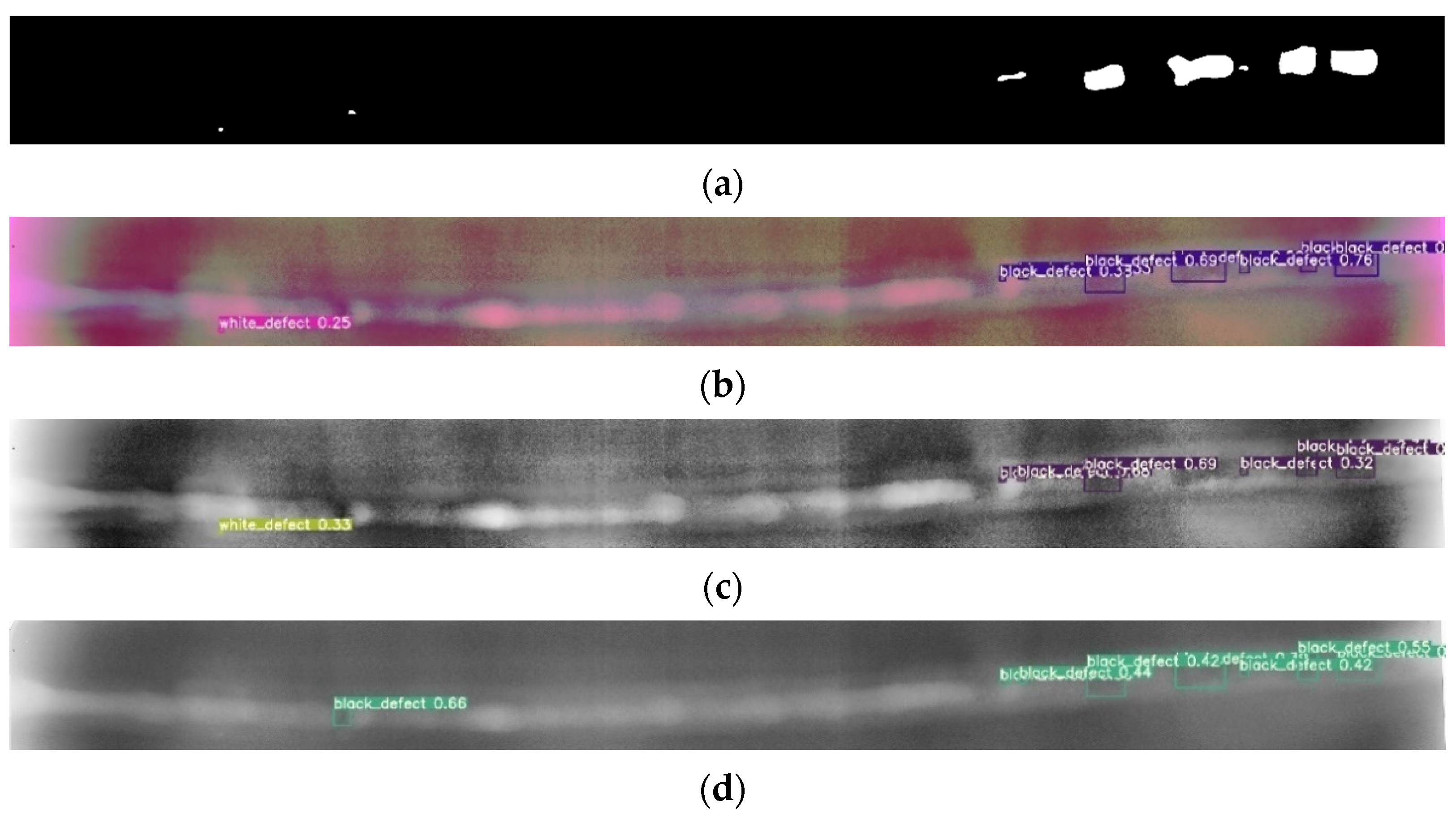
Figure 15a shows a mask image marked with welding defects, Figure 15b shows the detection image of the model trained with the preprocessed image, and Figure 15c shows the detection image of the model trained with the typical preprocessed image, and Figure 15d shows the detection image of the model trained with the raw image. Comparing the defect detection images for each model and the mask images with welding defects, one false negative in Figure 15b, two false negatives in Figure 15c, and two false negatives and one false positive in Figure 15d were found.

Table 3. mAP for the preprocessed and raw images.

		Image with Preprocessing Method we Proposed	Image with Typical Preprocessing Method	Raw Image
		AP
Training	Black defect	81.6%	78.9%	71.3%
	White defect	88.2%	85.1%	84.7%
Test	Black defect	48.3%	46.3%	43.5%
	White defect	54.0%	40.6%	38.1%
		mAP
Training		84.9%	82.0%	78.0%
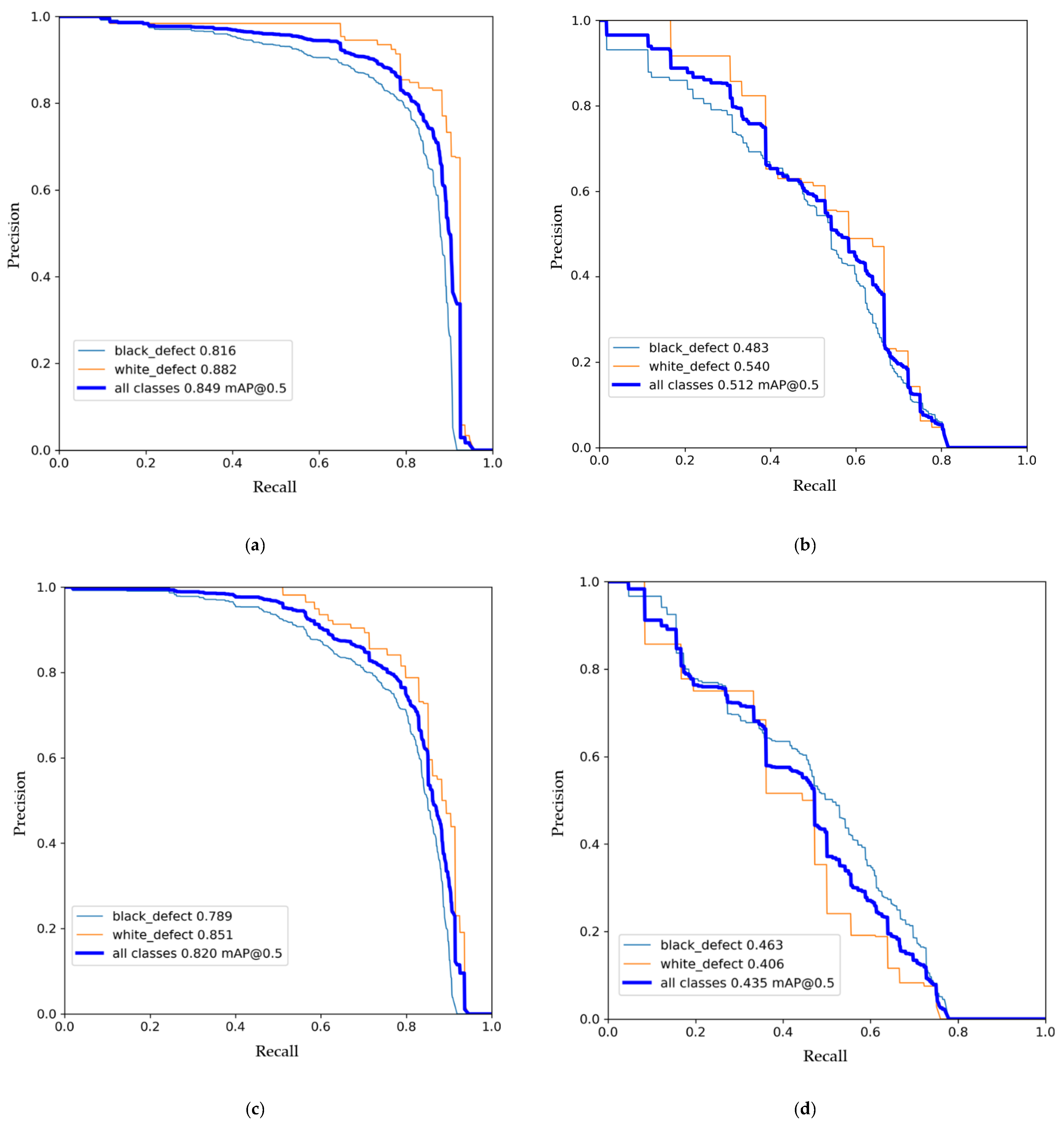
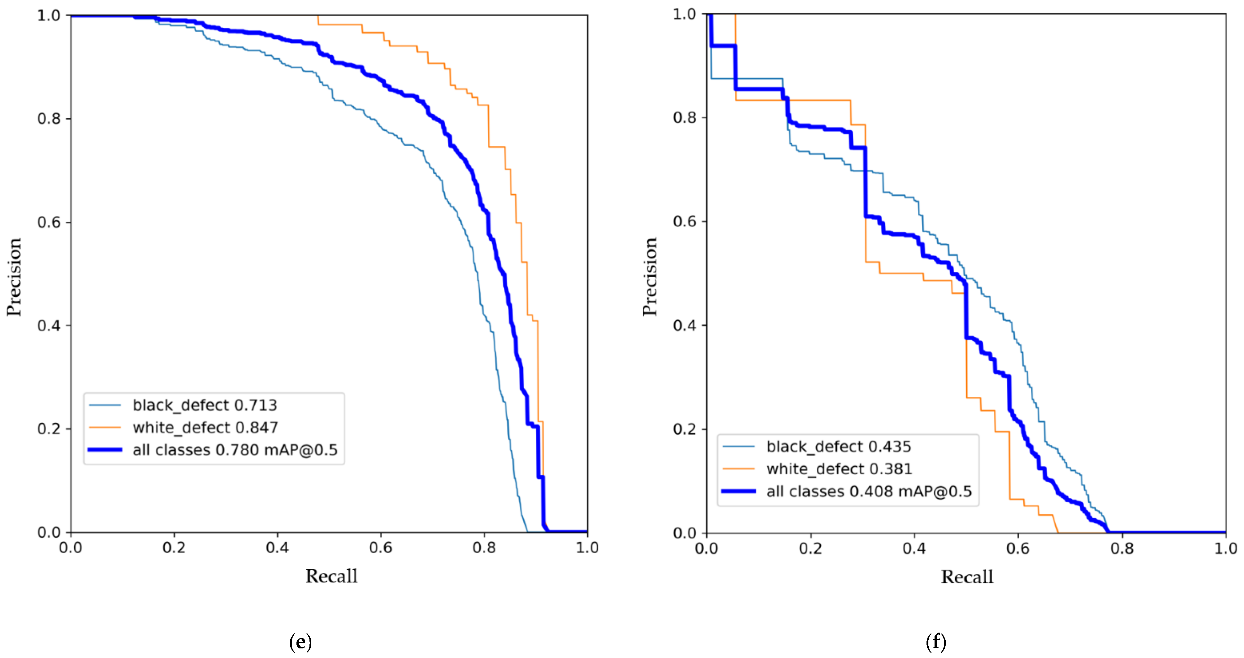
Test		51.2%	43.5%	40.8%

shows the mAP obtained through the PR curve for the training and test datasets of the preprocessed, typical preprocessed and raw image learning models in Figure 16. The mAP of the training data was 84.9% for the preprocessed image learning model, 82.0% for the typical preprocessed image learning model, and 78.0% for the raw image learning model. The mAP of the test data was 51.2%, 43.5% and 40.8%, respectively.

5. Conclusions

An image preprocessing method to be applied before the development of a detection algorithm for ship welding defects was developed by sequentially performing CLAHE, denoising, and thresholding of radiographic inspection images to increase the pixel intensity difference between the defect and background parts of the welding bead and to reveal the characteristics of the defect.

First, a large contrast effect was revealed by contrasting each defect according to the region using CLAHE. The sharpness of the image was then improved by denoising the image. To remove pixel values other than the defect and background parts of the welding image, a threshold was set, and the images were processed accordingly. Next, the final preprocessed images were obtained by concatenating the thresholded image for a welding defect with a low pixel value, the image threshold-processed by reversing the pixel values for a welding defect with a high pixel value, and the raw image to grayscale so that the pixel values had three channels.

The training mAP derived by training the YOLO algorithm with the images obtained through the preprocessing was 84.9%, whereas the training mAP derived by training the YOLO algorithm with the typical preprocessed image and raw image was 82.0%, 78.0%. Thus, the mAP of the model trained with the preprocessed image was 2.9% points higher than that of the typical preprocessed image learning model, and 6.9% points higher than that of the raw image learning model. Furthermore, the mAP for the test dataset of the preprocessed image learning model was 51.2%, whereas that for the test dataset of the typical preprocessed image learning model and for the test dataset of the raw image learning model was 43.5%, 40.8%, respectively. Thus, the mAP of the preprocessed image learning model was 7.7% points higher than that of the typical preprocessed image learning model, and 10.8% points higher than that of the raw image learning model.

Object detection algorithm technology is evolving, and the mAP is improving by approximately 3–10% per year [27]. This study achieved a comparable performance improvement by only preprocessing with data, rather than through the development of an object detection algorithm.

Image preprocessing of welding defects is a time-consuming process. The denoising after CLAHE in the preprocessing step improved the sharpness by removing several noises, but small defects were removed in some cases because the details of the image were lost. If the time requirement of preprocessing can be reduced, it should facilitate the dataset building process for the welding defect detection algorithm.

References

- Lee, S. Trend of Nondestructive Testing in Shipbuilding Industry. J. Weld. Join. 2010, 28, 5–8. [Google Scholar] [CrossRef] [Green Version]
- Dai, J.; Zhao, H.; Feng, X. Machine Vision; Science Press: Beijing, China, 2005. [Google Scholar]
- LeCun, Y.; Bengio, Y.; Hinton, G. Deep learning. Nature 2015, 521, 436–444. [Google Scholar] [CrossRef] [PubMed]
- Kim, D.H.; Boo, S.B.; Hong, H.C.; Yeo, W.G.; Lee, N.Y. Machine Vision-based Defect Detection Using Deep Learning Algorithm. Korean Soc. Nondestruct. Test. 2020, 40, 47–52. [Google Scholar] [CrossRef]
- Seo, J.B.; Jang, H.H.; Cho, Y.B. Analysis of Image Pre-processing Algorithms for Efficient Deep Learning. Korea Inst. Inf. Commun. Eng. 2020, 24, 161–164. [Google Scholar]
- Pan, H.; Pang, Z.; Wang, Y.; Wang, Y.; Chen, L. A new image recognition and classification method combining transfer learning algorithm and mobilenet model for welding defects. IEEE Access 2020, 8, 119951–119960. [Google Scholar] [CrossRef]
- Yang, L.; Wang, H.; Huo, B.; Li, F.; Liu, Y. An automatic welding defect location algorithm based on deep learning. NDT E Int. 2021, 120, 102435. [Google Scholar] [CrossRef]
- Hou, W.; Zhang, D.; Wei, Y.; Guo, J.; Zhang, X. Review on computer aided weld defect detection from radiography images. Appl. Sci. 2020, 10, 1878. [Google Scholar] [CrossRef] [Green Version]
- Thien, N.D.; Le Chi, C.; Ngoc, H.N. An approach to the automatic detection of weld defects in radiography films using digital image processing. In Proceedings of the 2017 International Conference on System Science and Engineering (ICSSE), Ho Chi Minh City, Vietnam, 21–23 July 2017; pp. 371–374. [Google Scholar]
- Pizer, S.M.; Amburn, E.P.; Austin, J.D.; Cromartie, R.; Geselowitz, A.; Greer, T.; ter Haar Romeny, B.; Zimmerman, J.B.; Zuiderveld, K. Zuiderveld, K. Adaptive histogram equalization and its variations. Comput. Vis. Graph. Image Process. 1987, 39, 355–368. [Google Scholar] [CrossRef]
- Cho, H.; Kye, H. The clip limit decision of contrast limited adaptive histogram equalization for X-ray images using Fuzzy logic. J. Korea Multimed. Soc. 2015, 18, 806–817. [Google Scholar] [CrossRef] [Green Version]
- Reza, A.M. Realization of the contrast limited adaptive histogram equalization (CLAHE) for real-time image enhancement. J. VLSI Signal Process. Syst. Signal 2004, 38, 35–44. [Google Scholar] [CrossRef]
- Majeed, A.R.; Awan, W.A.; ul Hassan, N.; Asghar, M.A.; Khan, M.J. Retinal Fundus Image Refinement with Contrast Limited Adaptive Histogram Equalization, Noise Filtration and Intensity Adjustment. In Proceedings of the 2020 IEEE 23rd International Multitopic Conference (INMIC), Bahawalpur, Pakistan, 5–7 November 2020; pp. 1–6. [Google Scholar]
- Buades, A.; Coll, B.; Morel, J.M. A non-local algorithm for image denoising. In Proceedings of the 2005 IEEE Computer Society Conference on Computer Vision and Pattern Recognition (CVPR’05), San Diego, CA, USA, 20–25 June 2005; Volume 2, pp. 60–65. [Google Scholar]
- Darbon, J.; Cunha, A.; Chan, T.F.; Osher, S.; Jensen, G.J. Fast nonlocal filtering applied to electron cryomicroscopy. In Proceedings of the 2008 5th IEEE International Symposium on Biomedical Imaging: From Nano to Macro, Paris, France, 14–17 May 2008; pp. 1331–1334. [Google Scholar]
- Sola, J.; Sevilla, J. Importance of input data normalization for the application of neural networks to complex industrial problems. IEEE Trans. Nucl. Sci. 1997, 44, 1464–1468. [Google Scholar] [CrossRef]
- Sønderby, C.K.; Espeholt, L.; Heek, J.; Dehghani, M.; Oliver, A.; Salimans, T.; Kalchbrenner, N. Metnet: A neural weather model for precipitation forecasting. arXiv 2020, arXiv:2003.12140. [Google Scholar]
- Zhao, L.; Peng, X.; Tian, Y.; Kapadia, M.; Metaxas, D. Learning to forecast and refine residual motion for image-to-video generation. In Proceedings of the European Conference on Computer Vision (ECCV), Munich, Germany, 8–14 September 2018; pp. 387–403. [Google Scholar]
- An, S.; Choi, Y.; Son, M.; Kim, K.H.; Jung, S.H.; Park, Y.Y. Short-Term Precipitation Forecasting based on Deep Neural Network with Synthetic Weather Radar Data. In Proceedings of the Korean Institute of Information and Communication Sciences Conference, Yeosu, Korea, 20–22 May 2021; pp. 43–45. [Google Scholar]
- Jang, J.; An, H.; Lee, J.H.; Shin, S. Construction of faster R-CNN deep learning model for surface damage detection of blade systems. J. Korea Inst. Struct. Maint. Insp. 2019, 23, 80–86. [Google Scholar]
- Redmon, J.; Divvala, S.; Girshick, R.; Farhadi, A. You only look once: Unified, real-time object detection. In Proceedings of the IEEE Conference on Computer Vision and Pattern Recognition, Las Vegas, NV, USA, 27–30 June 2016; pp. 779–788. [Google Scholar]
- Girshick, R. Fast r-cnn. In Proceedings of the IEEE International Conference on Computer Vision, Santiago, Chile, 7–13 December 2015; pp. 1440–1448. [Google Scholar]
- Rezatofighi, H.; Tsoi, N.; Gwak, J.; Sadeghian, A.; Reid, I.; Savarese, S. Generalized intersection over union: A metric and a loss for bounding box regression. In Proceedings of the IEEE/CVF Conference on Computer Vision and Pattern Recognition, Long Beach, CA, USA, 15–20 June 2019; pp. 658–666. [Google Scholar]
- Davis, J.; Goadrich, M. The relationship between Precision-Recall and ROC curves. In Proceedings of the 23rd International Conference on Machine Learning, Pittsburgh, PA, USA, 25–29 June 2006; pp. 233–240. [Google Scholar]
- Everingham, M.; Eslami, S.A.; Van Gool, L.; Williams, C.K.; Winn, J.; Zisserman, A. The pascal visual object classes challenge: A retrospective. Int. J. Comput. Vis. 2015, 111, 98–136. [Google Scholar] [CrossRef]
- Hassaballah, M.; Awad, A.I. Deep Learning in Computer Vision: Principles and Applications; CRC Press: Boca Raton, FL, USA, 2020. [Google Scholar]
- Zou, Z.; Shi, Z.; Guo, Y.; Ye, J. Object detection in 20 years: A survey. arXiv 2019, arXiv:1905.05055. [Google Scholar]
Figure 1.
Pixel redistribution.
Figure 2.
(a) Raw image and (b) image after CLAHE.
Figure 3.
Illustration of the difference between the background and defect parts by expanding the pixel distribution of the image through HE: (a) histogram of the raw image and (b) histogram of the image after CLAHE.
Figure 4.
Comparison of the image and the histogram by magnifying the parts of the image with and without NLM denoising: (a) non-denoised image, (b) denoised image, (c) histogram of the non-denoised image, and (d) histogram of the denoised image.
Figure 5.
Image with noise removed after applying CLAHE: (a) denoised image and (b) denoised and reversed image.
Figure 6.
Thresholding was performed to erase unnecessary parts of the background: (a) thresholded image and (b) reverse thresholded image.
Figure 7.
Image construction after converting the thresholded image, reverse thresholded image, and raw image to grayscale, so that the pixel values are composed of three channels: final preprocessed image.
Figure 8.
Method of organizing data.
Figure 9.
Basic structure of YOLO.
Figure 11.
Loss function using IoU.
Figure 12.
Loss function using GIoU.
Figure 13.
Pixel difference between the bead part and the welding defect part.
Figure 14.
(a) Loss of preprocessed image, (b) loss of typical preprocessed image and (c) loss of raw image.
Figure 15.
(a) Mask image for the location of welding defects, (b) example of preprocessed image test result, and (c) example of typical preprocessed image test result, and (d) example of raw image test result.
Figure 16.
(a) PR curve for the training dataset of the preprocessed image, (b) PR curve for the test dataset of the preprocessed image, (c) PR curve for the training dataset of the typical preprocessed image, (d) PR curve for the test dataset of the typical preprocessed image, (e) PR curve for the training dataset of the raw image, and (f) PR curve for the test dataset of the raw image.