
Factorial Analysis for Gas Leakage Risk Predictions from a Vehicle-Based Methane Survey


Abstract
:1. Introduction
- The main contribution of this paper is the novelty FA method combined with OE normalization to improve the accuracy of the results of standard ML algorithms by 6~10%.
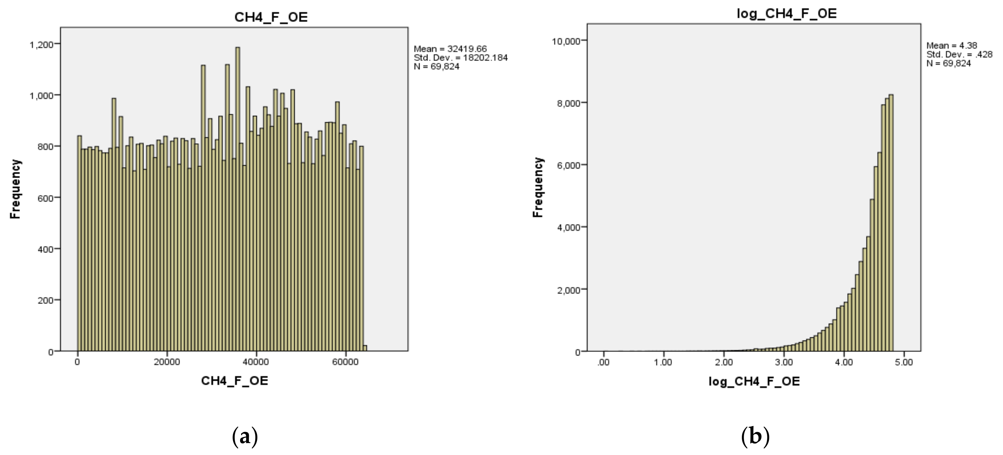
- Another advantage is that the data are normalized by the OE method, and logarithmic transformation is performed, theoretically resulting in a data distribution identical to that in earlier work [9]. Subsequently, imbalanced data were included in this gas data used to generate the gas leakage level given the k-mean clustering method.
- In addition, the study was also implemented using actual open data that had not previously been used with the ML algorithm, which future researchers will widely use for comparative research.
- It is also possible to use this method to create gas leakage data levels for air assessments in Korea.
- In practice, this level is considered a step forward in forecasting to determine leakages depending on the elements of environmental data information. Advances in the detection of gas leaks in everyday life can also help develop studies that accurately identify the health effects of gas leakages, suggesting the possibility of preventing such leaks and developing medical applications.
- Finally, the limitation of this study is that the multi-variable outlier detection method was not used in the data pre-processing. Our following study hoped that the feature selection method would improve the accuracy results after the multivariate outlier detection method was using Mahalanobis distance [10] and a deep autoencoder.
2. Related Work
3. Methodology
3.1. Factorial-Analysis-Based Feature Selection
3.2. Data analysis
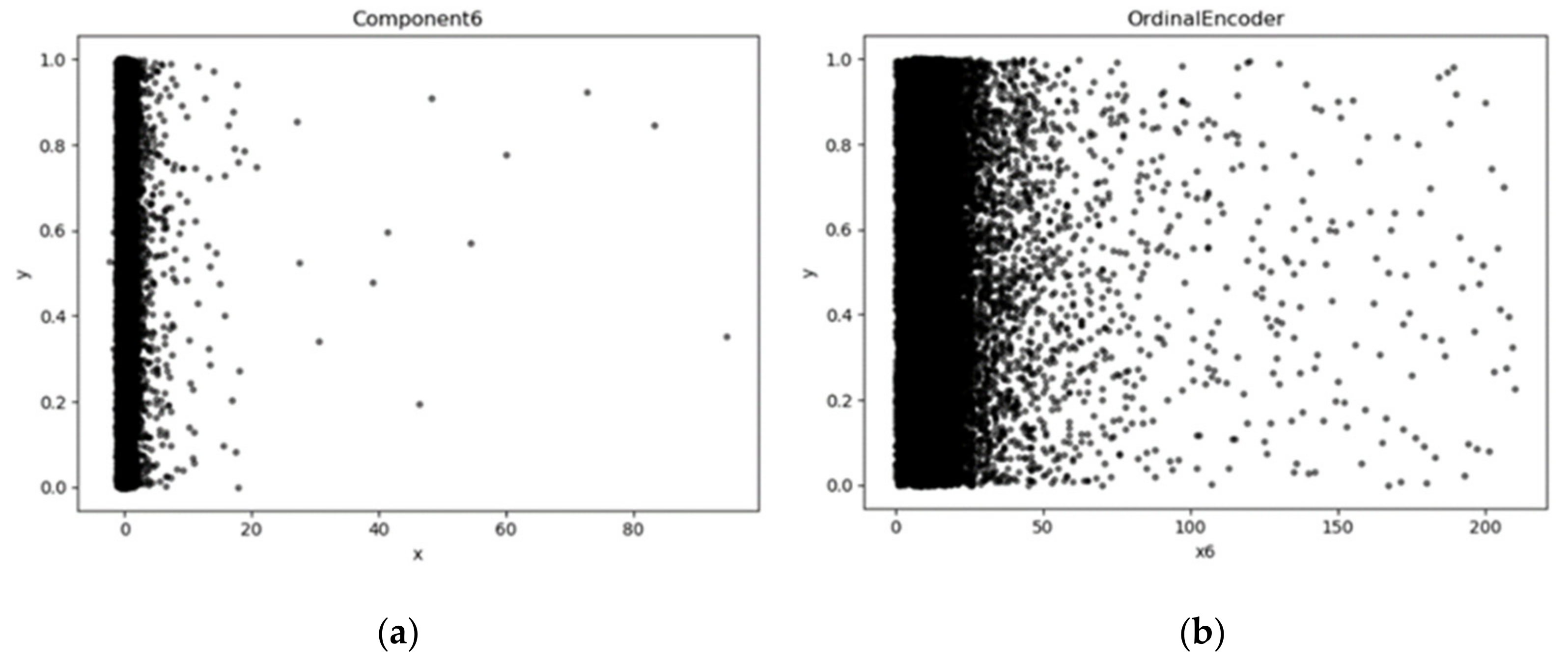
3.2.1. Data Normalization Using Ordinal Encoder and Log10 Transform
3.2.2. Data Labeling Using K-Means Clustering
4. Experimental Study
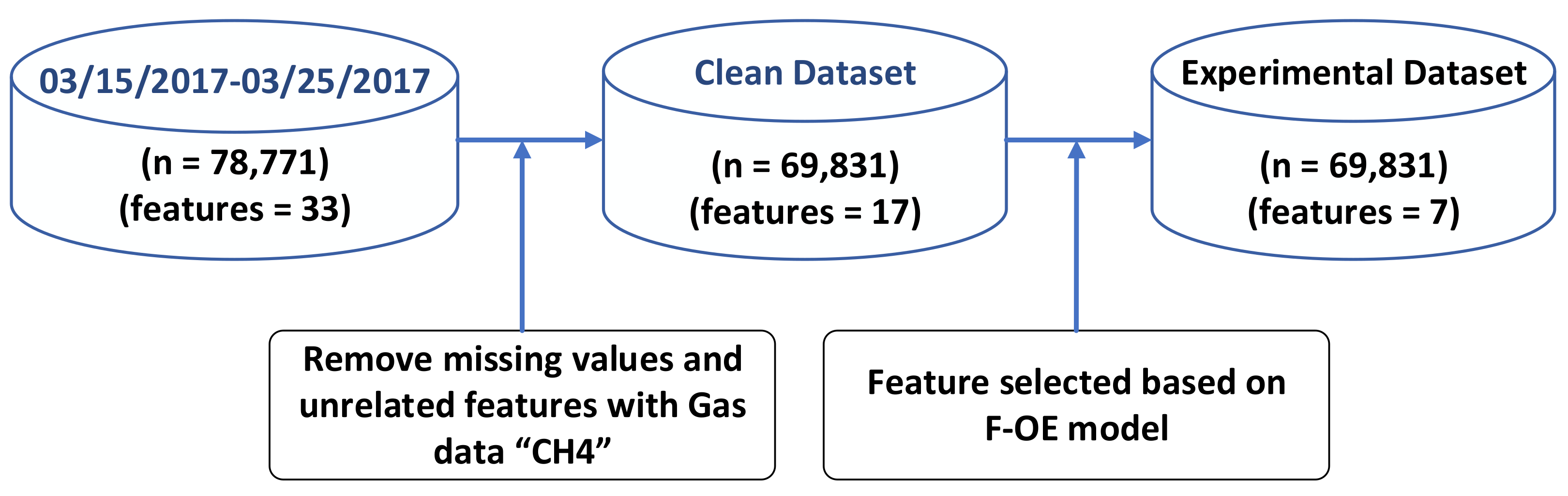
4.1. Experimental Dataset
4.2. Classifiers
4.3. Evaluation Metrics
5. Results and Discussion
6. Conclusions
Author Contributions
Funding
Institutional Review Board Statement
Informed Consent Statement
Conflicts of Interest
References
- Ministry of Public Safety and Security. 2019th Yearbook of Disaster, Ministry of Public Safety and Security; Ministry of Public Safety and Security: Sejong, Korea, 2019.
- Department for International Development. Live Data Page for Energy and Water Consumption. Available online: http://data.gov.uk/dataset/dfid-energy-and-water-consumption (accessed on 8 March 2021).
- Kim, Y.K.; Sohn, H.G. Disasters from 1948 to 2015 in Korea and power-law distribution. In Disaster Risk Management in the Republic of Korea; Springer: Singapore, 2017; pp. 77–97. [Google Scholar] [CrossRef]
- Deichmann, J.L.; Hernández-Serna, A.; Campos-Cerqueira, M.; Aide, T.M. Soundscape analysis and acoustic monitoring document impacts of natural gas exploration on biodiversity in a tropical forest. Ecol. Indic. 2017, 74, 39–48. [Google Scholar] [CrossRef] [Green Version]
- Zadkarami, M.; Safavi, A.A.; Taheri, M.; Salimi, F.F. Data driven leakage diagnosis for oil pipelines: An integrated approach of factor analysis and deep neural network classifier. Trans. Inst. Meas. Control 2020, 42, 2708–2718. [Google Scholar] [CrossRef]
- USDT. Leak Detection Technology Study for PIPES Act; Tech. Rep.; U.S. Department of Transportation: Washington, DC, USA, 2007.
- Bryce, P.; Jax, P.; Fang, J. Leak-detection system designed to catch slow leaks in offshore Alaska line. Oil Gas J. 2002, 100, 53–59. [Google Scholar]
- Behari, N.; Sheriff, M.Z.; Rahman, M.A.; Nounou, M.; Hassan, I.; Nounou, H. Chronic leak detection for single and multiphase flow: A critical review on onshore and offshore subsea and arctic conditions. J. Nat. Gas Sci. Eng. 2020, 11, 103460. [Google Scholar] [CrossRef]
- Weller, Z.D.; Yang, D.K.; Fischer, J.C. An open-source algorithm to detect natural gas leaks from mobile methane survey data. PLoS ONE 2019, 14, e0212287. [Google Scholar]
- Dashdondov, K.; Kim, M.H. Mahalanobis Distance Based Multivariate Outlier Detection to Improve Performance of Hypertension Prediction. Neural Process. Lett. 2021, 2, 1–3. [Google Scholar] [CrossRef]
- von Fischer, J.C.; Cooley, D.; Chamberlain, S.; Gaylord, A.; Griebenow, C.J.; Hamburg, S.P.; Salo, J.; Schumacher, R.; Theobald, D.; Ham, J. Rapid vehicle-based identification of location and magnitude of urban natural gas pipeline leaks. Environ. Sci. Technol. 2017, 51, 4091–4099. [Google Scholar] [CrossRef] [PubMed]
- Zachary, D.W.; Duck, K.Y.; von Joseph, C.F. Instruction for Processing Mobile Methane Survey Data to Detect Natural Gas Leaks; Colorado State University: Fort Collins, CO, USA, 2018; Available online: https://github.com/JVF-CSU/MobileMethaneSurveys/tree/master/Scripts/SampleRawData (accessed on 10 October 2018).
- Khongorzul, D.; Kim, M.H.; Lee, S.M. OrdinalEncoder based DNN for natural gas leak prediction. J. Korea Converg. Soc. 2019, 10, 7–13. [Google Scholar]
- Xue, P.; Jiang, Y.; Zhou, Z.; Chen, X.; Fang, X.; Liu, J. Machine learning-based leakage fault detection for district heating networks. Energy Build. 2020, 223, 110161. [Google Scholar] [CrossRef]
- Xu, Y.; Zhao, X.; Chen, Y.; Yang, Z. Research on a mixed gas classification algorithm based on extreme random tree. Appl. Sci. 2019, 9, 1728. [Google Scholar] [CrossRef] [Green Version]
- Lei, Y.; Jiang, W.; Jiang, A.; Zhu, Y.; Niu, H.; Zhang, S. Fault diagnosis method for hydraulic directional valves integrating PCA and XGBoost. Processes 2019, 7, 589. [Google Scholar] [CrossRef] [Green Version]
- Janizadeh, S.; Vafakhah, M.; Kapelan, Z.; Mobarghaee Dinan, N. Hybrid XGboost model with various Bayesian hyperparameter optimization algorithms for flood hazard susceptibility modeling. Geocarto Int. 2021, 21, 1–20. [Google Scholar] [CrossRef]
- Zhu, S.B.; Li, Z.L.; Zhang, S.M.; Liang, L.L.; Zhang, H.F. Natural gas pipeline valve leakage rate estimation via factor and cluster analysis of acoustic emissions. Measurement 2018, 125, 48–55. [Google Scholar] [CrossRef]
- Shamshirband, S.; Hadipoor, M.; Baghban, A.; Mosavi, A.; Bukor, J.; Várkonyi-Kóczy, A.R. Developing an ANFIS-PSO model to predict mercury emissions in combustion flue gases. Mathematics 2019, 7, 965. [Google Scholar] [CrossRef] [Green Version]
- Fagiani, M.; Squartini, S.; Gabrielli, L.; Severini, M.; Piazza, F. A statistical framework for automatic leakage detection in smart water and gas grids. Energies 2016, 9, 665. [Google Scholar] [CrossRef] [Green Version]
- Makonin, S.; Popowich, F.; Bartram, L.; Gill, B.; Bajic, I.V. AMPds: A public dataset for load disaggregation and eco-feedback research. In Proceedings of the 2013 IEEE Electrical Power Energy Conference, Halifax, NS, Canada, 21–23 August 2013; pp. 1–6. [Google Scholar]
- Chen, T.; Guestrin, C. Xgboost: A scalable tree boosting system. In Proceedings of the 22nd ACM Sigkdd International Conference on Knowledge Discovery and Data Mining, San Francisco, CA, USA, 13–17 August 2016; pp. 785–794. [Google Scholar]
- Zhang, M.L.; Pena, J.M.; Robles, V. Feature selection for multi-label naive Bayes classification. Inf. Sci. 2009, 179, 3218–3229. [Google Scholar] [CrossRef]
- Khongorzul, D.; Lee, S.M.; Kim, Y.K.; Kim, M.H. Image denoising methods based on DAECNN for medication prescriptions. J. Korea Converg. Soc. 2019, 10, 17–26. [Google Scholar] [CrossRef]
- Hemmati-Sarapardeh, A.; Hajirezaie, S.; Soltanian, M.R.; Mosavi, A.; Nabipour, N.; Shamshirband, S.; Chau, K.W. Modeling natural gas compressibility factor using a hybrid group method of data handling. Eng. Appl. Comput. Fluid Mech. 2020, 14, 27–37. [Google Scholar] [CrossRef] [Green Version]
- Mohammadi, M.R.; Hadavimoghaddam, F.; Pourmahdi, M.; Atashrouz, S.; Munir, M.T.; Hemmati-Sarapardeh, A.; Mosavi, A.H.; Mohaddespour, A. Modeling hydrogen solubility in hydrocarbons using extreme gradient boosting and equations of state. Sci. Rep. 2021, 11, 17911. [Google Scholar] [CrossRef]
- Quy, T.B.; Kim, J.M. Real-time leak detection for a gas pipeline using a k-NN classifier and hybrid ae features. Sensors 2021, 21, 367. [Google Scholar] [CrossRef]
- Quy, T.B.; Muhammad, S.; Kim, J.M. A reliable acoustic emission-based technique for the detection of a small leak in a pipeline system. Energies 2019, 12, 1472. [Google Scholar] [CrossRef] [Green Version]
- Zhou, M.; Zhang, Q.; Liu, Y.; Sun, X.; Cai, Y.; Pan, H. An integration method using kernel principal component analysis and cascade support vector data description for pipeline leak detection with multiple operating modes. Processes 2019, 7, 648. [Google Scholar] [CrossRef] [Green Version]
- Zhao, H.; Li, Z.; Zhu, S.; Yu, Y. Valve internal leakage rate quantification based on factor analysis and wavelet-BP neural network using acoustic emission. Appl. Sci. 2020, 10, 5544. [Google Scholar] [CrossRef]
- Xie, J.; Xu, X.; Dubljevic, S. Long range pipeline leak detection and localization using discrete observer and support vector machine. AIChE J. 2019, 65, e16532. [Google Scholar] [CrossRef]
- Melo, R.O.; Costa, M.G.; Costa, F.C.F. Applying convolutional neural networks to detect natural gas leaks in wellhead images. IEEE Access 2020, 8, 191775–191784. [Google Scholar] [CrossRef]
- Rui, X.; Qunfang, H.; Jie, L. Leak detection of gas pipelines using acoustic signals based on wavelet transform and Support Vector Machine. Measurement 2019, 146, 479–489. [Google Scholar] [CrossRef]
- Xie, Y.; Xiao, Y.; Liu, X.; Liu, G.; Jiang, W.; Qin, J. Time-frequency distribution map-based Convolutional Neural Network (CNN) model for underwater pipeline leakage detection using acoustic signals. Sensors 2020, 20, 5040. [Google Scholar] [CrossRef] [PubMed]
- Vapnik, V.N. The Nature of Statistical Learning Theory; Springer: New York, NY, USA, 1995. [Google Scholar]
- Nabipour, N.; Mosavi, A.; Baghban, A.; Shamshirband, S.; Felde, I. Extreme learning machine-based model for Solubility estimation of hydrocarbon gases in electrolyte solutions. Processes 2020, 8, 92. [Google Scholar] [CrossRef] [Green Version]


| Features | Mean | Std. Deviation | Communalities Extraction |
|---|---|---|---|
| CavityPressure | 139.99 | 0.0076 | 99.4 |
| CavityTemp | 45.02 | 0.1948 | 69.3 |
| DasTemp | 48.27 | 4.5963 | 79.9 |
| EtalonTemp | 44.71 | 0.0429 | 89.9 |
| WarmBoxTemp | 45.01 | 0.0359 | 88.0 |
| OutletValve | 28,652.2 | 402.65 | 86.6 |
| GPS_ABS_LAT | 33.5 | 0.0155 | 31.9 |
| WS_WIND_LON | 1.01 | 24.393 | 51.7 |
| WS_WIND_LAT | −5.65 | 11.604 | 49.2 |
| WS_COS_HEADING | −0.003 | 0.7081 | 54.7 |
| WS_SIN_HEADING | −0.033 | 0.6717 | 36.9 |
| WIND_N | 1.46 | 18.535 | 62.9 |
| WIND_E | −4.005 | 17.589 | 58.1 |
| WIND_DIR_SDEV | 25.22 | 24.215 | 51.9 |
| CAR_SPEED | 4.17 | 5.5035 | 57.8 |
| CH4 | 2.005 | 0.2032 | 83.2 |
| Features | Component | ||||||
|---|---|---|---|---|---|---|---|
| 1 | 2 | 3 | 4 | 5 | 6 | 7 | |
| DasTemp | 0.868 | ||||||
| OutletValve | 0.848 | ||||||
| GPS_ABS_LAT | |||||||
| WS_WIND_LAT | |||||||
| EtalonTemp | 0.943 | ||||||
| WarmBoxTemp | 0.931 | ||||||
| WIND_N | −0.783 | ||||||
| WS_WIND_LON | 0.688 | ||||||
| WS_SIN_HEADING | 0.507 | ||||||
| WIND_E | 0.682 | ||||||
| WIND_DIR_SDEV | 0.661 | ||||||
| WS_COS_HEADING | |||||||
| CavityTemp | 0.684 | ||||||
| CAR_SPEED | 0.590 | ||||||
| CH4 | 0.908 | ||||||
| CavityPressure | 0.997 | ||||||
| Class | Total | Train 70% | Test 30% |
|---|---|---|---|
| Low | 35,765 | 25,111 | 10,654 |
| Medium | 24,561 | 17,121 | 7440 |
| High | 9505 | 6649 | 2856 |
| Total | 69,831 | 48,881 | 20,950 |
| Algorithm | Parameters | Optimal Values |
|---|---|---|
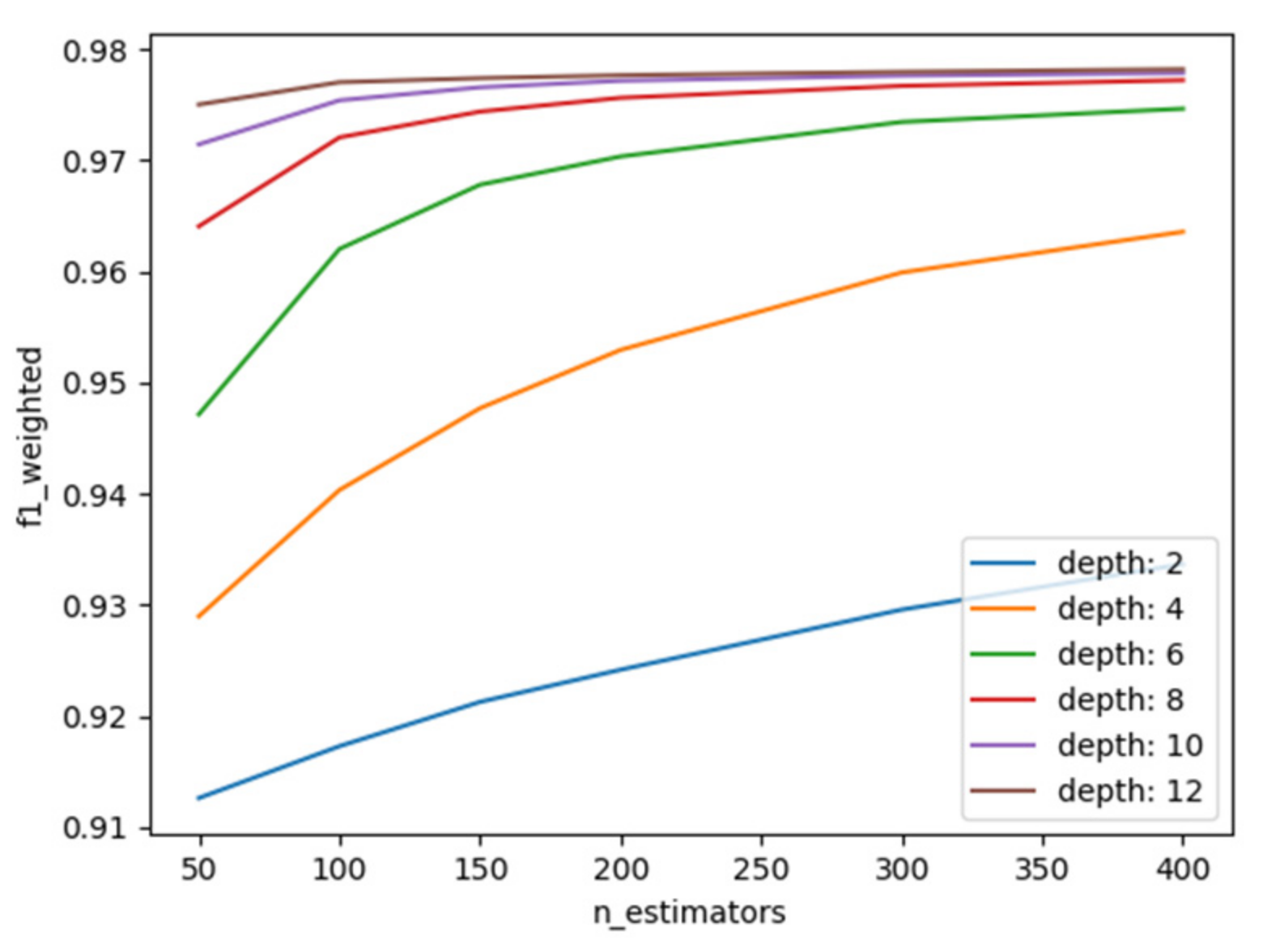
| XGBoost | n_estimators: The number of boosting stages to perform. Gradient boosting is robust to over-fitting; accordingly, a large number usually results in better performance. This was configured to be between 50 and 400 and increased in steps of 50. learning_rate: The learning rate shrinks the contribution of each tree according to the learning_rate value. max_depth: Maximum depth of the individual regression estimators. The maximum depth limits the number of nodes in the tree. We tune this parameter for the best performance; the best value depends on the interaction of the input variables. | n_estimators = 300, learning_rate = 0.1, max_depth = 12 |
| KNN | n_neighbors: Number of neighbors. It is configured between 2 and 30. | n_neighbors = 3 |
| DT | criterion: ‘gini’ for the Gini impurity and ‘entropy’ for the information gain measurements of the criterion of a split was used to identify the best decision tree splitting candidate. | criterion = ‘gini’ |
| RF | n_estimators: The number of trees in the forest. It was configured to be between 10 and 100 and increased in steps of 10. criterion: “gini” and “entropy” were used as splitting criteria. | n_estimators = 100, criterion = ‘gini’ |
| Algorithms | Accuracy | F1 | MSE | AUC | |
|---|---|---|---|---|---|
| 7 features with OE | F-OE-XGBoost | 95.141 | 0.957579 | 0.028226 | 96.29 |
| F-OE -KNN | 95.018 | 0.952601 | 0.031551 | 95.88 | |
| F-OE -DT | 90.859 | 0.937716 | 0.041496 | 94.78 | |
| F-OE -RF | 95.093 | 0.956036 | 0.029196 | 96.11 | |
| F-OE -NB | 65.709 | 0.731945 | 0.173381 | 76.16 | |
| 7 features | F-XGBoost | 94.993 | 0.955336 | 0.029722 | 96.17 |
| F-KNN | 93.079 | 0.947657 | 0.034163 | 95.07 | |
| F-DT | 56.678 | 0.678796 | 0.204025 | 72.82 | |
| F-RF | 69.709 | 0.703196 | 0.179618 | 74.02 | |
| F-NB | 70.916 | 0.762133 | 0.140000 | 76.74 | |
| 17 features | XGBoost | 88.382 | 0.896736 | 0.065044 | 83.71 |
| KNN | 84.902 | 0.850603 | 0.096150 | 79.39 | |
| DT | 80.267 | 0.857235 | 0.095768 | 82.14 | |
| RF | 88.702 | 0.896528 | 0.064185 | 82.86 | |
| NB | 64.821 | 0.658825 | 0.207160 | 56.49 |
Publisher’s Note: MDPI stays neutral with regard to jurisdictional claims in published maps and institutional affiliations. |
© 2021 by the authors. Licensee MDPI, Basel, Switzerland. This article is an open access article distributed under the terms and conditions of the Creative Commons Attribution (CC BY) license (https://creativecommons.org/licenses/by/4.0/).
Share and Cite
Dashdondov, K.; Song, M.-H. Factorial Analysis for Gas Leakage Risk Predictions from a Vehicle-Based Methane Survey. Appl. Sci. 2022, 12, 115. https://doi.org/10.3390/app12010115
Dashdondov K, Song M-H. Factorial Analysis for Gas Leakage Risk Predictions from a Vehicle-Based Methane Survey. Applied Sciences. 2022; 12(1):115. https://doi.org/10.3390/app12010115
Chicago/Turabian StyleDashdondov, Khongorzul, and Mi-Hwa Song. 2022. "Factorial Analysis for Gas Leakage Risk Predictions from a Vehicle-Based Methane Survey" Applied Sciences 12, no. 1: 115. https://doi.org/10.3390/app12010115