Article

A Hierarchical Feature-Based Methodology to Perform Cervical Cancer Classification

by
Débora N. Diniz
1,*,†,
Mariana T. Rezende
2,†,
Andrea G. C. Bianchi
1,
Claudia M. Carneiro
2,
Daniela M. Ushizima
3,
Fátima N. S. de Medeiros
4 and
Marcone J. F. Souza
1
1
Departamento de Computação, Universidade Federal de Ouro Preto (UFOP), Ouro Preto 35400-000, Brazil
2
Departamento de Análises Clínicas, Universidade Federal de Ouro Preto (UFOP), Ouro Preto 35400-000, Brazil
3
Computational Research Division, Lawrence Berkeley National Laboratory, Berkeley, CA 94720, USA
4
Departamento de Engenharia de Teleinformática, Universidade Federal do Ceará (UFC), Fortaleza 60020-181, Brazil
*
Author to whom correspondence should be addressed.
These authors contributed equally to this work.
Appl. Sci. 2021, 11(9), 4091; https://doi.org/10.3390/app11094091
Submission received: 30 March 2021 / Revised: 24 April 2021 / Accepted: 26 April 2021 / Published: 30 April 2021
(This article belongs to the Special Issue Computer Aided Diagnosis)

Abstract

:
Prevention of cervical cancer could be performed using Pap smear image analysis. This test screens pre-neoplastic changes in the cervical epithelial cells; accurate screening can reduce deaths caused by the disease. Pap smear test analysis is exhaustive and repetitive work performed visually by a cytopathologist. This article proposes a workload-reducing algorithm for cervical cancer detection based on analysis of cell nuclei features within Pap smear images. We investigate eight traditional machine learning methods to perform a hierarchical classification. We propose a hierarchical classification methodology for computer-aided screening of cell lesions, which can recommend fields of view from the microscopy image based on the nuclei detection of cervical cells. We evaluate the performance of several algorithms against the Herlev and CRIC databases, using a varying number of classes during image classification. Results indicate that the hierarchical classification performed best when using Random Forest as the key classifier, particularly when compared with decision trees, k-NN, and the Ridge methods.

1. Introduction

The World Health Organization recently estimated 605,000 new cases and 342,000 deaths from cervical cancer worldwide [1]. Over the years, the use of the Pap smear test for population-based cervical cytological screening has shown remarkable success in the early detection of such cancers; despite this, there is much to improve within this program [2,3].
The Papanicolaou exam, commonly known as the Pap smear, identifies pre-neoplastic changes in the cervix’s desquamated cells based on several cytomorphological and clinical criteria. The main criteria are based on nuclear characteristics, such as nuclear augmentation, irregularity of the nuclear membrane, nuclear hyperchromasia, and relation of the nucleus and cytoplasm sizes [4].
In the laboratory routine, a cytopathologist evaluates up to 300,000 cervical cells in a single smear [4]; also, the workload can reach 100 smears per day. The recommendation worldwide of the daily hours worked varies depending on the country: in Canada, it is 80 smears/day; in Brazil, it is 70 smears/day, and in the United States, it is 100 smears/day [5,6]. This scenario encompasses tiring and repetitive work that leads to errors inherent in human visual interpretation. Investigations conducted since before the 1990s show rates of 2% to 62% false-negatives in Pap test results [7,8,9,10,11].
To solve the limitations and improve the screening exams’ quality, computer vision and computer-aided systems are used to analyze Pap smear images, making the process more accurate and reliable [12]. One of the great difficulties in proposing such systems is the need for robust data from several real images of cervical cells, properly labeled by cytopathologists, using the widespread Bethesda System nomenclature. However, it comes up against the limitations of the existing Papanicolaou examination image datasets; these issues include synthetic images, images without classes images with pre-neoplastic or incomplete alteration, images with single cells, and liquid-based cytology images. The most widely used base, Herlev [13], has images with a single cell and a division into seven pre-neoplastic classes that do not follow the most-used nomenclature; the ISBI database [14] has simulated images and those without pre-neoplastic changes; SIPaKMeD [15] divides its images into five categories that differ from the Bethesda System.
Many authors have proposed solutions to this problem of detecting cervical cells, using synthetic databases or working with databases that do not represent the reality of conventional Pap smear images, in which there are many cells, often overlapping, in a single image [16,17,18,19,20,21,22,23,24]. Therefore, the investigation of methodologies capable of being applied in the real context of cervical cancer screening is still a great challenge.
Performing cell classification is one step in constructing a decision-aid tool for analyzing the Pap smear test. Some authors perform the cell classification with traditional machine learning [25,26,27], and others employ convolutional neural networks [17,23,28,29].
Diniz et al. [30] proposed a methodology using Simple Linear Iterative Clustering (SLIC), Density-Based Spatial Clustering of Applications with Noise (DBSCAN), and Iterated Local Search (ILS) algorithms to segment nuclei in synthetic images based on their morphologic features. Using the irace package, López-Ibánez et al. [31] and Diniz et al. [16] concluded that the important features for the methodology were minimum circularity, maximum intensity, and minimum area.
Ghoneim et al. [17] proposed a methodology based on the Shallow, VGG-16, and CaffeNet architectures to extract cervical cell characteristics. They also used the Extreme Learning Machine and Autoencoder to classify the cells into two or seven classes.
Lin et al. [18] presented a CNN-based method to classify cells based on their appearance and morphology. They analyzed different input images for the proposed method. They considered a 2-channel image, the nucleus and the cytoplasm masks, a 3-channel image, the RGB image, and the 5-channel image, which joins the 2-channel and 3-channel images. The authors showed with experiments that 5-channel input images improve the classification.
Di Ruberto et al. [32] analyzed different descriptors used to extract image features from seven databases representing different computer vision problems. They used a k-NN model to evaluate Hu, Legendre, and Zernike moments, Local Binary Patterns (LBP), and co-occurrence matrix features. The authors concluded that extracting the invariant moments from the Gray Level Co-occurrence Matrices (GLCM) improves their overall accuracy. They also observed that extracting the descriptors from RGB images is better than grayscale ones.
Ensemble methods are a process of consulting several classifiers before making a final decision and also have been used by many researchers in bioinformatics. Bora et al. [24] introduced an ensemble method that uses Least Squares Support Vector Machine (LSSVM), Multilayer Perceptron (MLP), and Random Forest (RF) to construct a decision model based on shape, texture, and color features.
Gómez et al. [19] made a comparison of several algorithms to classify cervical cancer cells into two classes: normal and abnormal. They used 20 morphologic features and found that the combinations of algorithms Bagging + MultilayerPerceptron and AdaBoostM1 + LMT were the best scenarios analyzed by them.
Lakshmi and Krishnaveni [20] presented a method to extract nuclei and cytoplasm features of Pap smear images. Attributes such as center, perimeter, area, and average intensity were considered. The method uses the expectation–maximization (EM) algorithm and a Gaussian mixture model (GMM). Finally, the authors state that the method can be used to determine the cancer stage and be efficient for classifying cervical cells that present low-grade squamous intraepithelial lesion (LSIL) and high-grade squamous intraepithelial lesion (HSIL).
Win et al. [21] applied a median filter to the images to remove noise and used Contrast Limited Adaptive Histogram Equalization (CLAHE) to enhance the contrast. The k-Means algorithm was implemented to segment the nucleus and cytoplasm regions of cervical cells. From these regions, 38 characteristics of texture, shape, and color were extracted. Attributes were selected using the Random Forest method. Next, the cells were classified into two and seven classes using the ensemble bagging method. The authors compared the approach with five classifiers (LD, SVM, k-NN, boosted trees, and bagged trees) and showed that their method performed better.
Hussain et al. [22] explore AlexNet, VGG-16, VGG-19, ResNet-50, ResNet-101, and GoogLeNet for the classification of cervical lesions. The authors also proposed an ensemble method of the three best models. They found GoogLeNet to be the best individual architecture, and they showed that the ensemble improved by using the AUC-ROC curve.
This article proposes the classification of pre-neoplastic cervical lesions based on features extracted from nuclei. The main contributions of this work can be summarized as:
  • investigation of handcrafted and biological features of nuclei images;
  • proposal and analysis of a hierarchical classification with Random Forest to perform state-of-the-art cell nuclei classification;
  • decision aid resource to decrease professionals’ workload and increase the Pap smear result’s reliability;
  • comparison of oversampling techniques to balance data;
  • introduction of the segmentation cervix collection of the CRIC Searchable Image database;
  • statistical comparison of different hierarchical classifiers.
The outline of the paper is as follows. Section 2 exhibits the materials and methods considered. Section 3 displays the computational experiments and their results and discussion. Finally, Section 4 presents the conclusions of this work.

2. Materials and Methods

This section presents the materials and methods considered. Section 2.1 presents the cervical cell databases, Herlev and CRIC, used for lesion classification. Section 2.2 exhibits how the features were extracted and analyzes the correlation between the handcrafted and biological nuclei features. Section 2.3 presents the classification groups of each database used in the experiments. Section 2.4 shows the oversampling techniques analyzed in the experiments. Section 2.5 points out the classifier methods used. Finally, Section 2.6 shows the hierarchical classification structure proposed for nuclei classification.

2.1. Database

This work deals with two databases of cervical cells: (i) Herlev, well known and used in the literature, and (ii) CRIC, a new database with nucleus and cell segmentation results in smear images.
The Herlev database [13] (
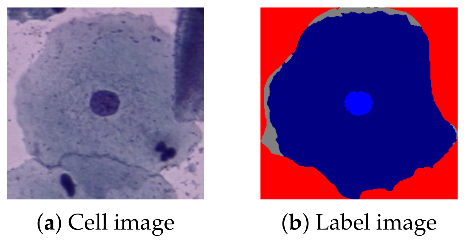
http://mde-lab.aegean.gr/index.php/downloads (accessed on 24 January 2021)) is collected at the Department of Pathology of Herlev University Hospital and the Department of Automation at the Technical University of Denmark. It consists of 917 single cervical cell images, divided into seven classes: superficial squamous epithelial; intermediate squamous epithelial; columnar epithelial; mild, moderate, and severe squamous non-keratinizing dysplasia; and squamous cell carcinoma in situ intermediate. All images also have a label of their regions, nuclei, and cytoplasm. Figure 1 shows a Herlev example image (a) and its label (b).
The CRIC Searchable Image Database (https://database.cric.com.br/ (accessed on 24 March 2021)) comprises cervical cell images and it is being developed by the Center for Recognition and Inspection of Cells (CRIC) and aims to support the Pap smear analysis. It covers cervical cells of conventional cytology, based on the standardized and most-used worldwide nomenclature in the diagnosis area, the Bethesda System nomenclature.
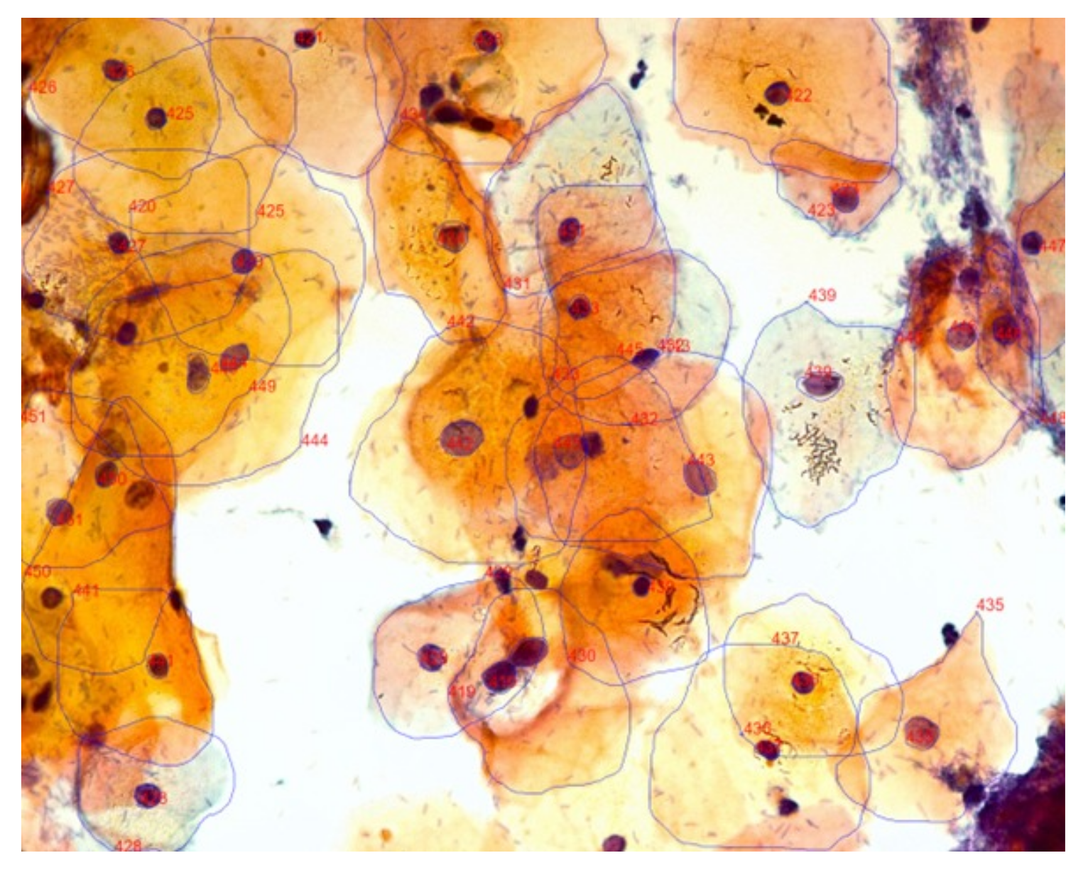
Currently, the CRIC database is divided into two collections: one containing only the marking of the cell’s center (classification) and another containing the segmentation of the cell’s nucleus and cytoplasm. In both cases, each cell also has its classification. Only the segmentation collection will be used in this work since the nucleus region’s delimitation will be important for the methodology used. There are 400 images obtained from Pap smears, with 3233 segmentations. Figure 2 presents an example of a segmentation image.
Table 1 shows each database division, indicating the nuclei’s categories and classifications. The number of nuclei in each class is also shown.
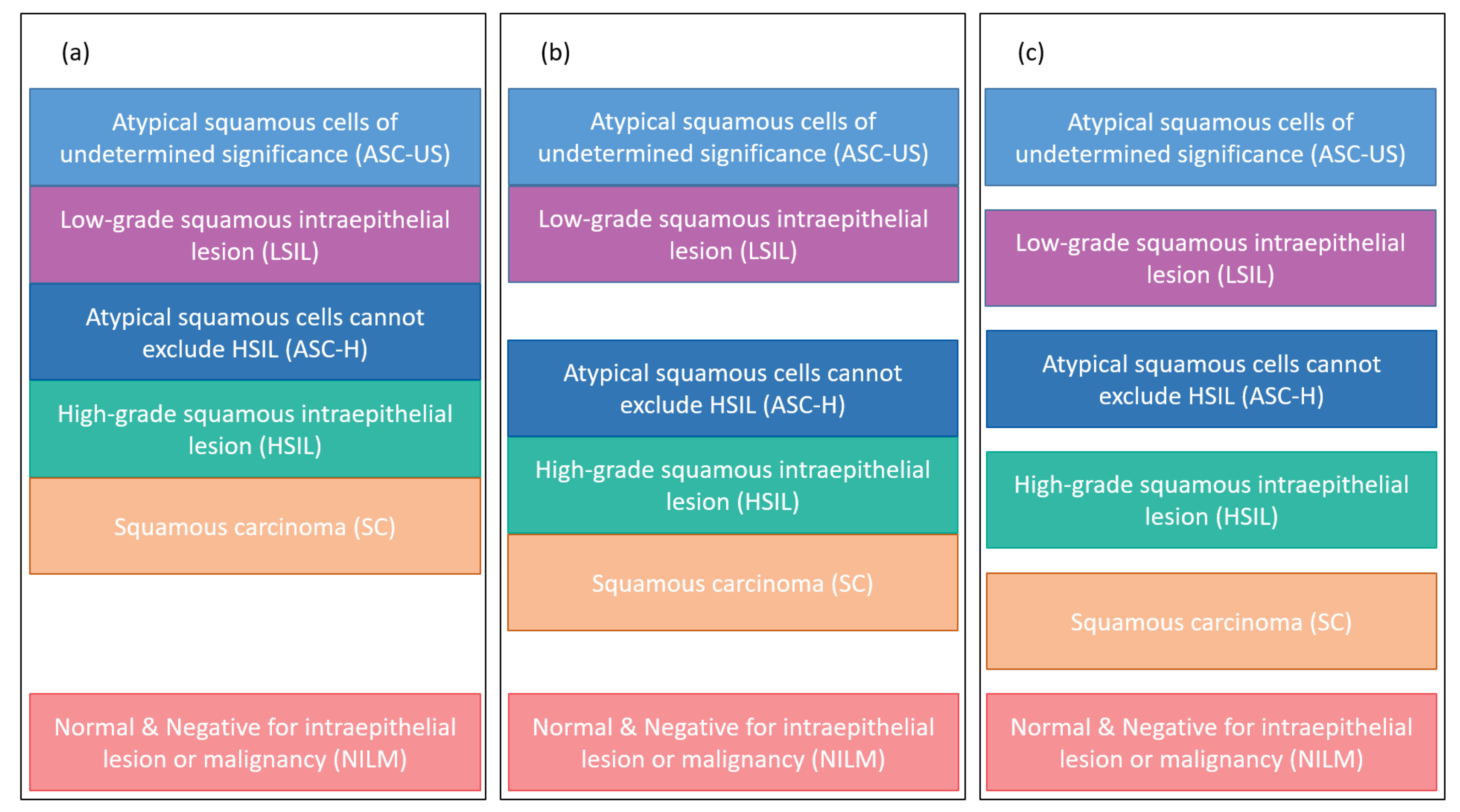
In 1941, George N. Papanicolaou created the first classification system for normal and abnormal cells (class I, II, III, IV, and V). The second system was created by James Reagan in 1953, separating the abnormal cells into mild, moderate, severe dysplasias, and carcinoma in situ. In 1967, Ralph Richart proposed the division into CIN I, CIN II, and CIN III (Cervical Intraepithelial Neoplasia). To standardize the terminologies, in 1988, the ”Bethesda System” was developed and approved by the National Cancer Institute in the USA; the system underwent reviews in 1991, 2001, and 2014. With this new nomenclature system, the current terms for the classification of abnormal squamous cells are ASC-US, LSIL, ASC-H, HSIL, SC [33,34].
Herlev’s database uses the second classification system developed in 1953, while the CRIC base uses the most current classification system, the Bethesda System. In this sense, comparing the terminologies, mild dysplasia corresponds to LSIL, and moderate, severe dysplasia and carcinoma in situ corresponds to HSIL. Therefore, Herlev does not include the classifications of classes ASC-US, ASC-H, and SC used in the laboratory routine today.
Our proposal uses information from the segmented nucleus to perform the classification of cells.

2.2. Biological versus Computational Features

As mentioned before, during the screening examination in a cytology laboratory, the cytopathologist manually analyzes optical images of cervical cells. Visual analysis is related to human interpretation of cervical smears, and even with many detailed procedures and routines, it is susceptible to errors of interpretation.
During the analysis, the cytopathologist assesses the variation in the smear cells’ cytomorphological features. Some examples of this variation are the increase in the nucleus/cytoplasm ratio, the nuclear membrane irregularity, the nucleus hyperchromasia, and the chromatin granularity. All of them provide guidance on reporting of cytologic findings in cervical cytology in agreement with the Bethesda System [4,34].
Errors related to diagnostic interpretation happen when the cytopathologist either recognizes altered cells, but wrongly classifies them, or does not recognize them at all. Both situations may be attributed to the lack of experience of the professional, variation in the appearance of cytomorphological features, or workload, which affects the subjectivity of the process [35,36,37].
Our proposal extracts and evaluates morphological and texture characteristics related to the cell nucleus, correlated to the Bethesda System’s visual interpretation. The computational results can guide the cell classification systems and assist the lesion diagnosis and interpretation, diminishing error results.
The methodology starts with a feature extraction of each nucleus segmented in the database. The following algorithms were employed: Region Props, Haralick’s features, Local Binary Patterns (LBP), Threshold Adjacency Statistics (TAS), Zernike moments, and Gray Level Co-occurrence Matrix (GLCM). All were implemented in Python, in which Region Props and GLCM are from the scikit-image package [38], and the others are from the Mahotas package [39]. Unlike Di Ruberto et al. [32], we also include morphological and other texture features.
First, Region Props [40,41,42,43] was used to extract the values of the morphological features of nuclei, such as (a) circularity; (b) minimum, mean, and maximum intensities; (c) area; (d) bounding box, filled, and convex hull image areas; (e) perimeter; (f) Euler number; (g) extent; (h) minor and major axis; (i) eccentricity; and (j) solidity.
Next, Haralick’s texture features [44] were extracted. These features are: (a) angular second moment; (b) contrast; (c) correlation; (d) variance; (e) inverse difference moment; (f) sum average; (g) sum entropy; (h) entropy; (i) difference variance; (j) difference entropy; (k) measure of correlation 1; (l) measure of correlation 2.
The Local Binary Patterns (LBP) [45], a set of texture features, were also extracted. The advantage of these features is that they are insensitive to orientation and lighting.
The Threshold Adjancency Statistics (TAS) [46] features were also considered in the classification. They are used to differentiate images of distinct subcellular localization quickly and with high accuracy.
The Zernike moment [47] features were extracted and considered in the proposed methodology because they measure how the mass is distributed in the region. Finally, the Gray Level Co-occurrence Matrices [44] are texture features extracted that consider the pixels’ spatial relation.
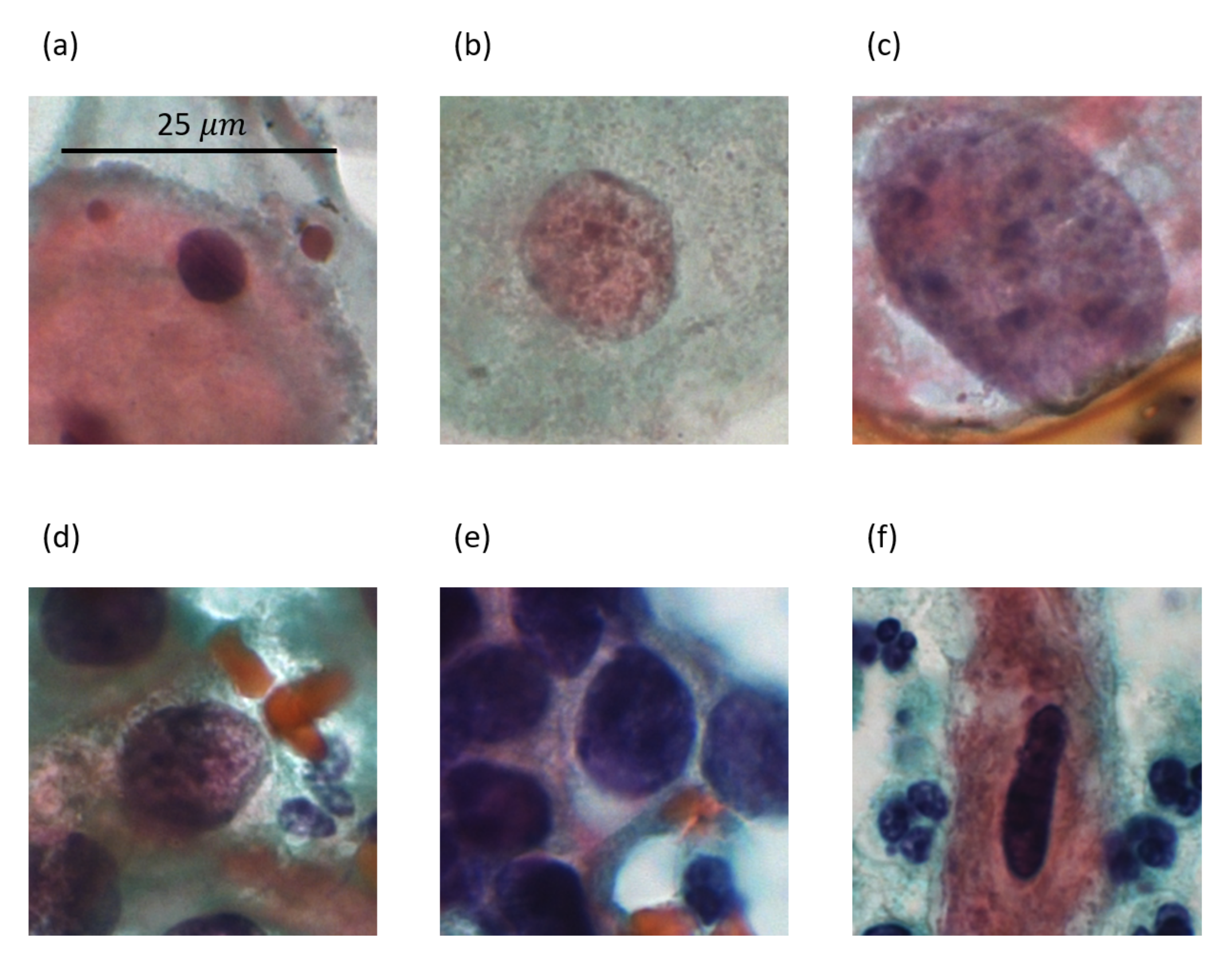
Figure 3 shows a sample image for each type of lesion present in the CRIC database, and Table 2 presents some feature values extracted from the images in Figure 3. These features are area, eccentricity (eccent.), circularity (circ.), maximum intensity (max. int.), and contrast.
We extracted features inspired by the ones that a cytopathologist would use to perform the classification, manually. Morphological features such as area, perimeter, extent, and eccentricity are important because they are related to the nuclear size, which characterizes one of the fundamental biological criteria for differentiating abnormal cells from normal ones. For example, ASC-US interpretation requires that the cells in question demonstrate nuclei approximately 2.5 to 3 times the area of the nucleus of a normal intermediate squamous cell (approximately 35 μm 2 ) or twice the size of a squamous metaplastic cell nucleus (approximately 50 μm 2 ). The cells interpreted as ASC-H are the size of metaplastic cells with nuclei that are up 2.5 times larger than normal. Nuclear enlargement more than three times the area of normal intermediate nuclei characterizes LSIL. HSIL often contains relatively small basal-type cells with nuclear augmentation. The characteristic cells of carcinoma (SC) vary markedly in the area but usually show karyomegaly. Table 2 shows that the area feature has a behavior as observed by cytopathologists, in which the normal cell has the smallest area value and there is an increase in the value according to its lesion.
Another biologically relevant feature is the nuclear membrane shape, as abnormal cells have different degrees of irregularity. ASC-US shows minimal variation in the nuclear shape, while LSIL presents a contour of nuclear membrane ranging from smooth to very irregular with notches. ASC-H and HSIL show irregular nuclear contour, with anisokaryosis of HSIL being more pronounced. Carcinoma cells may show very marked nuclear pleomorphism (bizarre forms). As a whole, abnormal cells may have multinucleation, or variations in the circular shape of a normal cell’s nucleus. This work considered morphological features related to these characteristics (nuclear contour and multinucleation), such as circularity, eccentricity, and minor and major axis. Table 2 shows eccentricity and circularity values that provide examples of features used in this work to measure the nuclear membrane’s shape as they would typically be analyzed by cytopathologists. The eccentricity measures the nuclei irregularity, while the circularity value represents how circular the nuclei are. Analyzing the images in Figure 3, the less circular nucleus is the SC, and it has the smallest value for the feature (0.462). Simultaneously, the most irregular nucleus is also the SC, and it has the biggest eccentricity value (0.952).
Nuclear hyperchromasia and irregular chromatin distribution are essential biological characteristics for categorizing cells as abnormal. These characteristics also assist in differentiation among ASC-US, LSIL, ASC-H, and HSIL. Moreover, the morphological features directly related to these characteristics are minimum, mean, and maximum intensities, solidity, contrast, mass distribution in the region (Zernike moments), and a set of texture features such as Local Binary Patterns, Haralick features, and Gray Level Co-occurrence Matrices. Table 2 shows the maximum intensity and the contrast (Haralick feature) values. With attributes of intensity (minimum, maximum, and medium) and texture, it is possible to estimate the chromatin distribution analyzed by the cytopathologist in the manual analysis.
A total of 232 attributes of the cervical cell nuclei were extracted and considered in this work. A quick analysis of the attribute selection indicated that all attributes used brought benefits to the classification task; thus, all of them were used in our proposal for the nuclei classification.

2.3. Classification Groups

As shown in Table 1, the database images can be classified according to their category (normal/abnormal) or their classification (7 classes in Herlev and 6 classes in CRIC).
Based on cytopathologists’ analysis of Herlev’s data, this work proposes a classification of the data into five classes for abnormal cells. Note that once a cell is classified as normal, it is not necessary to further distinguish its particular type. Thus, the classes superficial squamous epithelial, intermediate squamous epithelial, and columnar epithelia can be grouped as normal cells. Figure 4 shows the possible classification groups for the Herlev database. Figure 4a presents the 2-class group, Figure 4b the 5-class group, and Figure 4c the 7-class group.
Concerning CRIC, another possible classification task is grouping images into three classes: normal, low-grade lesion (ASC-US, and LSIL), and high-grade lesion (ASC-H, HSIL, and SC) cells. This classification is feasible due to their common disease follow-up. Women diagnosed with low-grade cell changes should repeat the exam after a certain period, according to her age, while the ones diagnosed with high-grade lesions should be referred for colposcopy followed by a biopsy [48]. Figure 5 shows the CRIC classification groups considered in this work’s computational experiments. Figure 5a exposes the 2-class group, Figure 5b the 3-class group, and Figure 5c the 6-class group.

2.4. Oversampling

In classification problems, a database is imbalanced when the difference between the amount of data of classes is large [49]. Classification algorithms are often sensitive to imbalance, which means that they tend to value classes with more data and ignore classes with fewer data [50,51]. It is possible to observe in Table 1 that the databases considered in this work are not balanced, so balancing techniques were analyzed.
The first used technique is the Synthetic Minority Oversampling Technique (SMOTE) [52], which creates artificial sample data based on neighboring interpolation to oversample the minority class. This technique considers the k-nearest neighbors for each sample x i of the minority class and creates a synthetic sample x n e w as follows:
x n e w = x i + ( x ^ i x i ) × δ .
In Equation (1), x ^ i corresponds to a random value of the k neighbors of x i and δ is a random number in the interval [0,1]. The new sample datum x n e w is a point on the edge that connects x i and x ^ i .
Another technique was the Borderline-SMOTE [53]. The difference between the Borderline-SMOTE and the original SMOTE is that the Borderline-SMOTE only oversamples the borderline examples of the minority class, while SMOTE oversamples through all the examples from the minority class.
Finally, the third technique studied is SVM SMOTE. This technique differs from the others because it uses the support vectors to generate a Support Vector Machine (SVM) classifier to approximate the class boundaries.
All these three techniques were implemented in Python using the imbalanced-learn package [54], and their results were compared according to accuracy.

2.5. Methods

We implemented eight classifiers to perform the nuclei classification. The classifiers considered were: AdaBoost [55,56], Decision Tree (DT) [57], Gaussian Naive-Bayes(GNB), k-Nearest Neighbors (k-NN) [58], Multi-Layer Perceptron (MLP) [59], Nearest Centroid (NC) [60], Random Forest (RF) [61], and Ridge [62]. However, only the four best classifiers are explicitly presented in this work.

2.5.1. Decision Tree (DT)

A Decision Tree [57] is a supervised method to perform classifications supported by data descriptions based on tree-structural patterns. For the Decision Tree, the input and the goal variables do not need a previous relationship. Moreover, it can handle data at different scales [63].

2.5.2. k-NN

The k-NN [58] is a supervised learning method in which, when a new instance needs to be classified, its distance to all neighbors is calculated and given the label of the nearest k-neighbors. In this way, the generalization and the prediction are only made when a new instance needs to be classified (lazy). The distance used in the method is the Euclidian distance between points p and q, given by d p , q , calculated as follows:
d p , q = i = 1 n ( p i q i ) 2 .
In Equation (2), n represents the number of features.

2.5.3. Random Forest (RF)

The Random Forest [61] is an ensemble learning method that uses multiple decision trees for decision making. In classification problems, the label defined by most decision trees is the label given to the new instance.

2.5.4. Ridge

The Ridge [62] classifier converts the label data to solve the problem with a regression method. In prediction, the highest value is accepted as a target class. For multiclass classification, multi-output regression is applied.

2.6. Hierarchical Classification

Some classification problems present hierarchical relations between classes, indicating that it is possible to divide the problem into sub-problems of less complexity that, when combined, reach the classification expected by the whole problem. These problems are known as hierarchical classification problems.
Here, we address a hierarchical classification problem because it can be reduced into a normal and abnormal classification followed by deeper classifications to discover the nuclei type. 
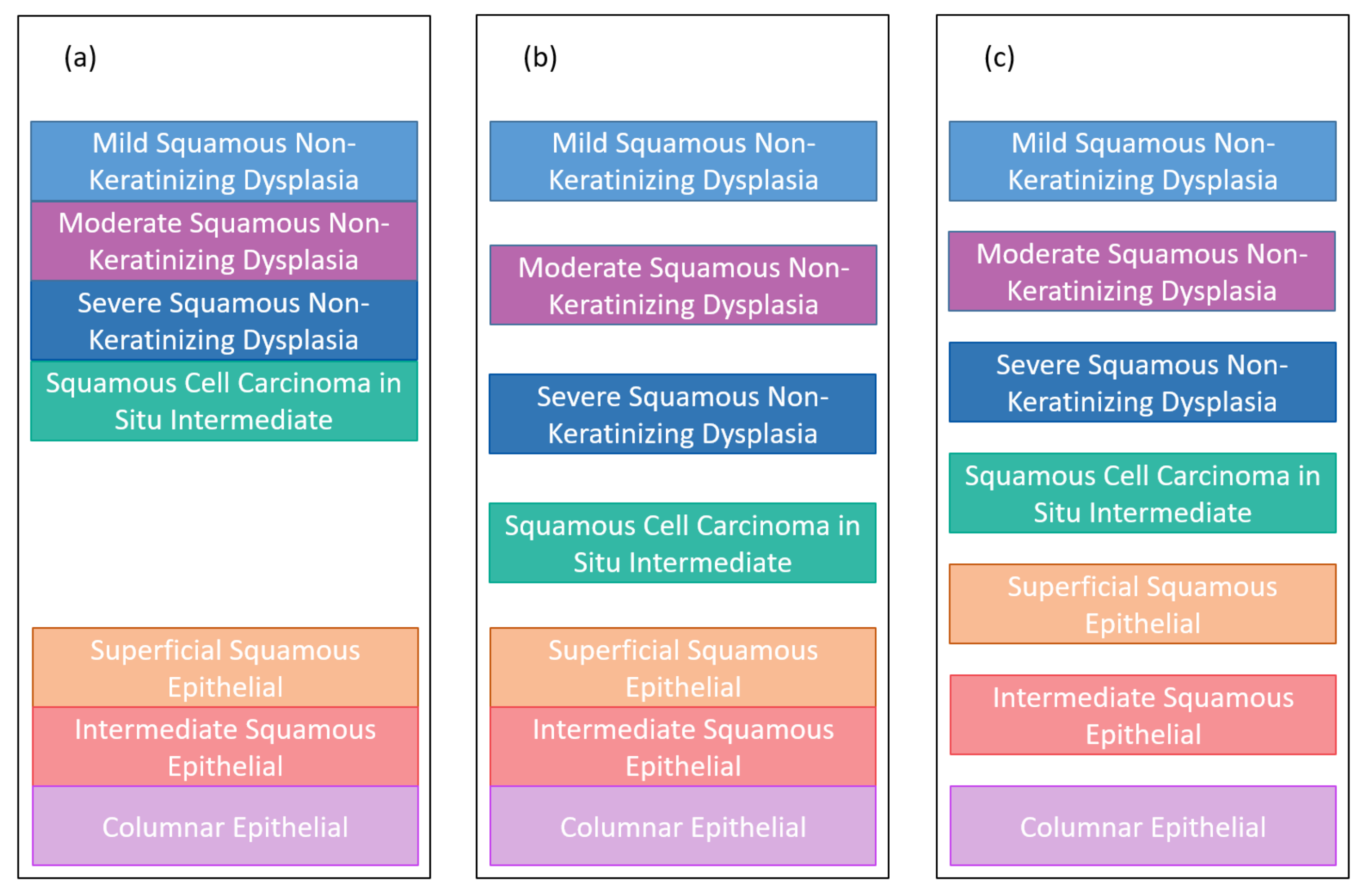
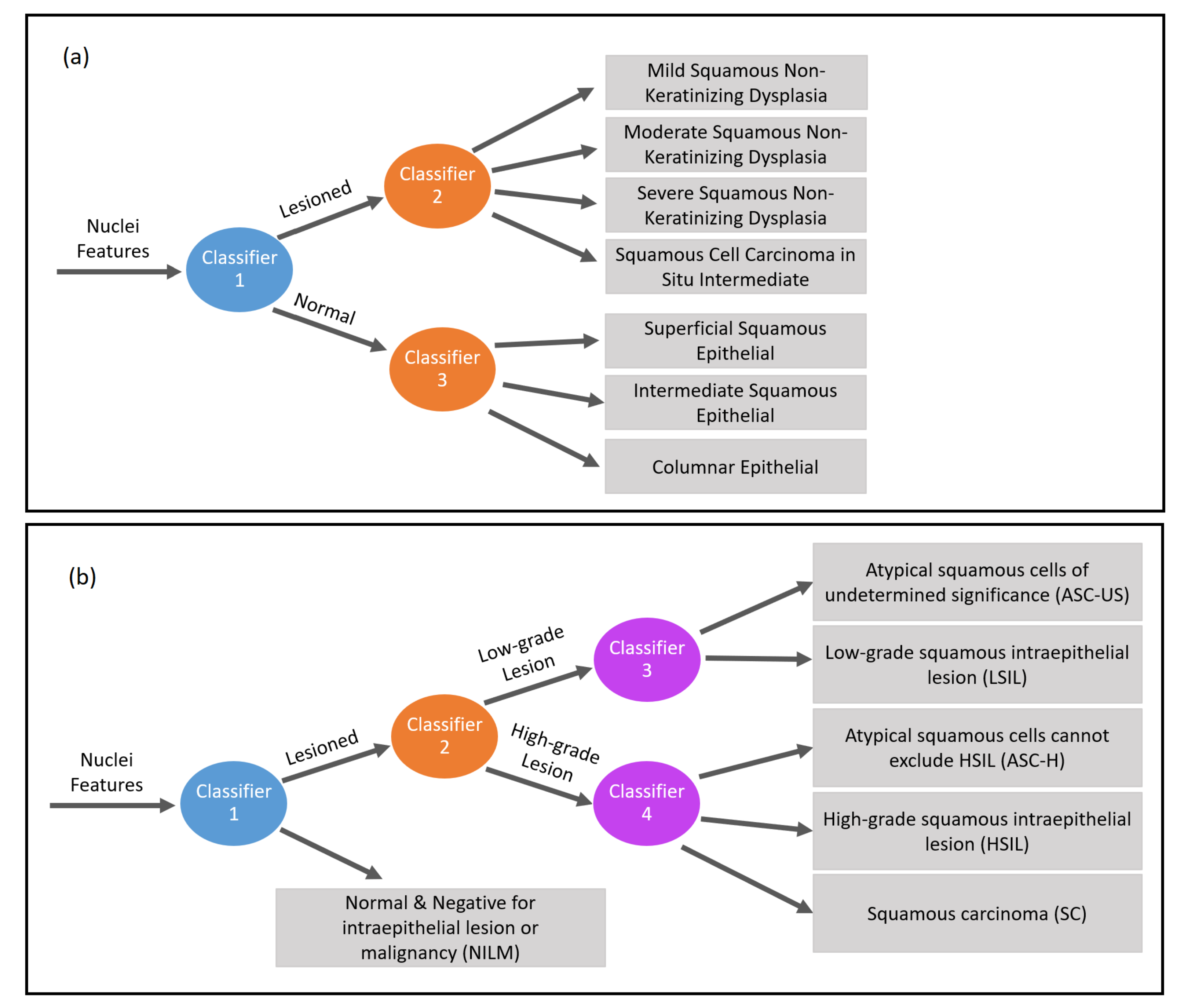
Figure 6 presents the hierarchical classification proposed in this work to classify nuclei features. Figure 6a shows the hierarchical classification of Herlev nuclei, while Figure 6b shows the hierarchical classification of CRIC nuclei.
Considering the Herlev data (Figure 6a), the data can be classified first (with classifier 1 in blue) between normal and abnormal and, subsequently, the lesion can be classified (with classifier 2 in orange) into four other classes (mild squamous non-keratinizing dysplasia, moderate squamous non-keratinizing dysplasia, severe squamous non-keratinizing dysplasia, and squamous cell carcinoma in situ intermediate), and the normal ones can be classified (with classifier 3 in orange) into another three classes (superficial squamous epithelial, intermediate squamous epithelial, columnar epithelial). Therefore, the 2-class classification requires only classifier 1. In turn, the 5-class classification requires classifiers 1 and 2, while the 7-class classification requires the three classifiers.
Considering the CRIC database data (Figure 6b), the data can be classified (with classifier 1 in blue) into normal and abnormal. The lesion can be classified (with classifier 2 in orange) into low-grade lesion and high-grade lesion, which are then classified (with classifiers 3 and 4 in purple) according to their lesion’s type. Thereby, the 2-class classification applies classifier 1; the 3-class, classifiers 1 and 2; and the 6-class, the four classifiers.

3. Experiments and Results

This section discusses the experiments developed to evaluate the hierarchical classification proposed. The experiments were performed on a computer with an Intel Core i7-8700 processor with a 3.20GHz processor, 16GB RAM, and a Windows 64-bit operating system. The hierarchical classification proposed uses the programming language Python, version 3.7.9. Codes are available at https://github.com/agcbianchi/AppliedScience-Feature.
Dhurandhar and Dobra [64] investigated cross-validation performance and presented explanations concerning varying sample size, number of folds, and the correlation between input and output attributes. They pointed out that 10- and 20-fold cross-validation worked best for small datasets. Thus, our experiments applied the 10-fold cross-validation. All the results correspond to the average of the 10-fold cross-validation.

3.1. Performance Metrics

Initially, the number of true positives (TP), true negatives (TN), false positives (FP), and false negatives (FN) was calculated. TP and TN are the numbers of positive and negative classes correctly predicted, while FP and FN are the numbers of positive and negative classes incorrectly predicted.
Table 3 shows the metrics used to measure performance of the hierarchical classification proposed.

3.2. Oversampling Results

Table 4 shows the performance results obtained using the balanced techniques and without any oversampling applied to the CRIC data. The 6-class classification is the most challenging; therefore, it was used in this experiment, aiming to provide greater differentiation in the results. As can been seen in Table 4, any oversampling technique improves the classification, but the best technique observed was the Borderline-SMOTE. For this reason, the Borderline-SMOTE was used as the oversampling technique in the experiments carried out. We only used this oversampling technique in the training data. The test set remained unchanged, guaranteeing the classification results’ credibility. The balancing techniques applied to the Herlev database performed similarly to the CRIC database, so these results were not presented.
Before balancing the data from the Herlev database with the Borderline-SMOTE technique, there were in the training base: 67 superficial squamous epithelial data; 63 intermediate squamous epithelial data; 83 epithelial columnar data; 164 mild squamous non-keratinizing dysplasia data; 132 moderate squamous non-keratinizing dysplasia data; 178 severe squamous non-keratinizing dysplasia data; and 135 squamous cell carcinoma in situ intermediate data. The largest class size (severe squamous non-keratinizing dysplasia with 178 data) was used as a reference size for balancing the data. Thus, after balancing, each of the seven classes comprised 178 data. These results were used in the 2-class balancing to allow all classes to be represented within the groups. In the 2-class balancing, we group the four abnormal classes, resulting in 712 (=4 × 178) abnormal cells, with data equally distributed among the four classes. The group of normal classes resulted in 534 (=3 × 178) data. Finally, we balanced the normal and abnormal groups so that they had the same number of samples.
In the CRIC database, there were 776 NILM data, 258 ASC-US, 539 LSIL, 483 ASC-H, 787 HSIL, and 70 SC. Thus, analogous to Herlev data balancing, to balance the CRIC data, we chose the reference size as 787, the most frequent class, HSIL. At the end of the balancing, each of the six classes was left with the same number of data. The 6-class balancing was also used for the 2- and 3-class balancing, aiming at the classes’ representativeness within the groups. Thus, the abnormal group resulted in 3935 (=5 × 787) data, and the normal one 787 (=1 × 787). We employed a new balancing such that the two groups (normal and abnormal) were left with 3935 data. Finally, the high-grade lesion group resulted in 2361 (=3 × 787) data, and the low-grade group in 1574 (=2 × 787) data in the 3-class balancing. These last two groups were again balanced, and finally, both comprised 2361 data.

3.3. Hierarchical Classification Results

Table 5 presents the results of precision, recall, F1, accuracy, and specificity for the 2-class, 5-class, and 7-class hierarchical classification of Herlev database nuclei images. The 7-class classification without hierarchy allows us to analyze and determine if the hierarchical classification improves the task. The best results are highlighted in bold. It is possible to observe that the RF classifier performs better than k-NN, Ridge, and DT, considering all metrics and number of classes. The results also reveal that the hierarchical methodology improves the classification.
In turn, Table 6 shows the results of 2-class, 3-class, 6-class hierarchical classification, and 6-class classification without a hierarchy of the CRIC database nuclei images. These results are similar to those for Herlev: our findings show that the RF is the best classifier, and the hierarchical methodology improves the classification. In RF, an ensemble learning technique [61], multiple decision trees are combined in a committee, known as boosting [65], whose final performance is better than the base classifiers. Each decision tree is trained with different features and is responsible for predicting diverse data in the classifier. Thus, the decision boundary becomes more stable and accurate with more trees. Simultaneously, the unpruned and diverse trees result in a high resolution in the feature space and a smoother decision boundary between the classes. These essential characteristics of RF, combined with the nonlinearity correlation of features, contribute to the good classification prediction [66].

3.4. Statistical Analysis

The statistical analysis aims to verify whether there is a statistically significant difference between the implemented algorithms’ results.
Initially, we used the Shapiro–Wilk test [67] with a significance level of 0.05 to verify whether the normal distribution can approximate the probability distribution of the classifiers’ results. It was found that the results obtained in all metrics do not follow a normal distribution.
For this reason, the Kruskal–Wallis non-parametric test [68] was chosen to determine whether the results obtained suggest that the samples are from different populations or are just random variations among random samples from the same population.
Thus, the best classifier found in the experiments, the RF, was compared pair-wise with the other classifiers using the non-parametric Kruskal–Wallis test with a significance level of 0.05 to check if there was a statistical difference between RF and the other classifiers concerning all performance metrics.
Table 7 shows the p-value results obtained in the Kruskal–Wallis test when comparing the RF results with those of k-NN, Ridge, and DT for 2-class, 3-class, and 7-class hierarchical classification, and 7-class classification without hierarchy using the Herlev database. The results highlighted in bold have the same distribution as the RF results (p-value > 0.05). Table 7 reveals that in 7-class hierarchical classification, the Ridge results of accuracy and specificity have the same distribution of the RF results.
In turn, Table 8 presents the p-value results obtained in the Kruskal–Wallis test when comparing the RF results with those of k-NN, Ridge, and DT for 2-class, 3-class, and 6-class hierarchical classification and 6-class classification without hierarchy using the CRIC database. As no p-value was higher than 0.05, it can be concluded that the RF statistically outperformed all other classifiers that classified the data from the CRIC database, considering all metrics.

3.5. Comparison with Literature

Table 9 presents the precision, recall, F1, accuracy, and specificity values obtained by the best method found in these experiments, the RF hierarchical classification, and other literature methods. Blank fields indicate that the literature methods did not report the respective metrics results. The best result of each metric is highlighted in bold. As can be seen in Table 9, the proposed RF hierarchical classifier obtained the best values of precision and F1, as well as achieving high recall, accuracy, and specificity when compared to the other methods in 2-class classification. In the 5-class and 7-class classification, the proposed RF hierarchical classifier obtained the best values of all metrics considered.

4. Conclusions

This work proposes a hierarchical classification methodology to classify nuclei of Pap smear images using handcrafted features. As mentioned before, in the cytopathologist’s routine, image analysis is entirely manual and subjective, a tiring and monotonous task. The proposal performs a computational screening procedure capable of excluding irrelevant nuclei images to identify possible lesions and reduce the number of images analyzed visually by the cytopathologist. The reduction of the professional workload helps to focus attention on the analysis of relevant images, decreasing false-negative rates.
The experiment indicates that hierarchical classification improves the results when compared with those without hierarchy. Considering the Herlev database, the results outperform the literature methods for 5-class and 7-class classification concerning the precision, recall, F1, accuracy, and specificity metrics. For the 2-class classification, our RF hierarchical method achieves the best results for two of the five metrics and had competitive results in the other metrics. Analyzing the metrics in which our method does not present the best result, we realize that the best result comes from a different method from the literature. However, even the best result for the specific metric performs poorly in all other metrics when compared to our method.
Additionally, this work introduces the CRIC segmentation cervix collection and presents 2-class, 3-class, and 6-class classification results considering precision, recall, F1, accuracy, and specificity metrics.
The present findings of cell nuclei classification suggest enhancing our understanding of the handcrafted features used in the machine learning algorithm. The hypothesis that features should be inspired in the biological criteria for differentiating abnormal cells from normal ones proved to be a feasible solution. The feature vector included a combination of nuclear contour shape morphologies with chromatin distribution (texture), and all attributes were used in the classification task.
We tested eight machine learning traditional classifier methods to perform the nuclei classification and chose the four best ones (Decision Tree, k-NN, Random Forest, and Ridge) to report their results in this work concerning the hierarchical classification proposed. A statistical analysis shows that the Random Forest is the best one to classify nuclei images of the Herlev and CRIC databases regardless of the number of classes.

Author Contributions

Conceptualization, D.N.D., M.T.R., A.G.C.B., C.M.C., D.M.U., F.N.S.d.M. and M.J.F.S.; Data curation, D.N.D., M.T.R., A.G.C.B., C.M.C. and M.J.F.S.; Formal analysis, D.N.D., M.T.R., A.G.C.B., C.M.C. and M.J.F.S.; Funding acquisition, A.G.C.B., C.M.C., D.M.U. and M.J.F.S.; Investigation, D.N.D., M.T.R., A.G.C.B., C.M.C., D.M.U., F.N.S.d.M. and M.J.F.S.; Methodology, D.N.D., M.T.R., A.G.C.B., C.M.C. and M.J.F.S.; Project administration, A.G.C.B., C.M.C. and M.J.F.S.; Resources, A.G.C.B., C.M.C. and M.J.F.S.; Software, D.N.D.; Supervision, A.G.C.B., C.M.C. and M.J.F.S.; Validation, D.N.D., M.T.R., A.G.C.B., C.M.C. and M.J.F.S.; Visualization, D.N.D. and M.T.R.; Writing—original draft, D.N.D. and M.T.R.; Writing—review and editing, D.N.D., M.T.R., A.G.C.B., C.M.C., D.M.U., F.N.S.d.M. and M.J.F.S. All authors have read and agreed to the published version of the manuscript.

Funding

This work was funded by the Coordenação de Aperfeiçoamento de Pessoal de Nível Superior—Brazil (CAPES)—Finance Code 001 (88882.459660/2019-01), Fundação de Amparo à Pesquisa do Estado de Minas Gerais (FAPEMIG, grants PPM/CEX/FAPEMIG/676-17, and PPSUS-FAPEMIG/APQ-03740-17), Conselho Nacional de Desenvolvimento Científico e Tecnológico (CNPq, grants 303266/2019-8, 06/2015-306396/2015-7, 06/2019 305895/2019-2, 304673/2011-0, 308947/2020-7, 401120/2013/9), Pró-Reitoria de Pesquisa e Inovação: PROPI/UFOP-19/2020, 23109.000928/2020-33, 23109.000929/2020-88, Moore-Sloan Foundation, and Office of Science, of the U.S. Department of Energy under Contract No. DE-AC02-05CH11231.

Institutional Review Board Statement

Not applicable.

Informed Consent Statement

Not applicable.

Data Availability Statement

The datasets used in this work are available from the CRIC Searchable Image Database (https://database.cric.com.br (accessed on 24 March 2021)) and the Herlev Database (https://mde-lab.aegean.gr/index.php/downloads (accessed on 24 January 2021)).

Acknowledgments

The authors would like to thank the Universidade Federal de Ouro Preto (UFOP), the Center for Recognition and Inspection of Cells (CRIC), the Group of Optimization and Algorithms (GOAL), and the eXtented Reality 4 Good (XR4GoodLab) for supporting this research.

Conflicts of Interest

The authors declare no conflict of interest.

Abbreviations

The following abbreviations are used in this manuscript:
ASC-HAtypical Squamous Cells cannot exclude HSIL
ASC-USAtypical Squamous Cells of Undetermined Significance
CLAHEContrast Limited Adaptive Histogram Equalization
CRICCenter for Recognition and Inspection of Cells
DTDecision Tree
EMExpectation–maximization
FNFalse Negative
FPFalse Positive
GLCMGray Level Co-occurrence Matrix
GMMGaussian Mixture Model
HSILHigh-grade Squamous Intraepithelial Lesion
ILSIterated Local Search
k-NNk-Nearest Neighbors
LBPLocal Binary Patterns
LSILLow-grade Squamous Intraepithelial Lesion
LSSVMLeast Square Support Vector Machine
MLPMultilayer Perceptron
NILMNegative for Intraepithelial Lesion or Malignancy
RFRandom Forest
SCSquamous Carcinoma
SLICSimple Linear Iterative Clustering
SMOTESynthetic Minority Oversampling TEchnique
SVMSupport Vector Machine
TASThreshold Adjacency Statistics
TNTrue Negative
TPTrue Positive

References

  1. Sung, H.; Ferlay, J.; Siegel, R.L.; Laversanne, M.; Soerjomataram, I.; Jemal, A.; Bray, F. Global cancer statistics 2020: GLOBOCAN estimates of incidence and mortality worldwide for 36 cancers in 185 countries. CA Cancer J. Clin. 2021, 68, 394–424. [Google Scholar]
  2. Koonmee, S.; Bychkov, A.; Shuangshoti, S.; Bhummichitra, K.; Himakhun, W.; Karalak, A.; Rangdaeng, S. False-negative rate of papanicolaou testing: A national survey from the Thai society of cytology. Acta Cytol. 2017, 61, 434–440. [Google Scholar] [CrossRef] [PubMed]
  3. Sachan, P.L.; Singh, M.; Patel, M.L.; Sachan, R. A study on cervical cancer screening using pap smear test and clinical correlation. Asia-Pac. J. Oncol. Nurs. 2018, 5, 337. [Google Scholar] [CrossRef] [PubMed]
  4. Wilbur, D.; Nayar, R. Bethesda 2014: Improving on a paradigm shift. Cytopathology 2015, 26, 339–342. [Google Scholar] [CrossRef]
  5. Miller, A.B.; Nazeer, S.; Fonn, S.; Brandup-Lukanow, A.; Rehman, R.; Cronje, H.; Sankaranarayanan, R.; Koroltchouk, V.; Syrjänen, K.; Singer, A.; et al. Report on consensus conference on cervical cancer screening and management. Int. J. Cancer 2000, 86, 440–447. [Google Scholar] [CrossRef]
  6. Mody, D.R.; Davey, D.D.; Branca, M.; Raab, S.S.; Schenck, U.G.; Stanley, M.W.; Wright, R.; Arbyn, M.; Beccati, D.; Bishop, J.W.; et al. Quality assurance and risk reduction guidelines. Acta Cytol. 2000, 44, 496–507. [Google Scholar] [CrossRef]
  7. Gay, J.; Donaldson, L.; Goellner, J. False-negative results in cervical cytologic studies. Acta Cytol. 1985, 29, 1043–1046. [Google Scholar]
  8. Bosch, M.; Rietveld-Scheffers, P.; Boon, M. Characteristics of false-negative smears tested in the normal screening situation. Acta Cytol. 1992, 36, 711. [Google Scholar]
  9. Naryshkin, S. The false-negative fraction for Papanicolaou smears. Arch. Pathol. Lab. Med. 1997, 121, 270. [Google Scholar]
  10. Franco, R.; Amaral, R.G.; Montemor, E.B.L.; Montis, D.M.; Morais, S.S.; Zeferino, L.C. Fatores associados a resultados falso-negativos de exames citopatológicos do colo uterino. Rev. Bras. Ginecol. Obstet. 2006, 28, 479–485. [Google Scholar] [CrossRef]
  11. Silva, G.P.F.; Cristovam, P.C.; Vidotti, D.B. O impacto da fase pré-analítica na qualidade dos esfregaços cervicovaginais. Rev. Bras. An. Clín. 2017, 49, 135–140. [Google Scholar]
  12. William, W.; Ware, J.; Habinka, A.; Obungoloch, J. A review of Image Analysis and Machine Learning Techniques for Automated Cervical Cancer Screening from pap-smear images. Comput. Methods Programs Biomed. 2018, 164, 15–22. [Google Scholar] [CrossRef]
  13. Jantzen, J.; Norup, J.; Dounias, G.; Bjerregaard, B. Pap-smear benchmark data for pattern classification. In Proceedings of the Nature Inspired Smart Information Systems (NiSIS 2005), Albufeira, Portugal, 4–5 October 2005; pp. 1–9. [Google Scholar]
  14. Lu, Z.; Carneiro, G.; Bradley, A.P.; Ushizima, D.M.; Nosrati, M.S.; Bianchi, A.G.C.; Carneiro, C.M.; Hamarneh, G. Evaluation of Three Algorithms for the Segmentation of Overlapping Cervical Cells. IEEE J. Biomed. Health Inform. 2017, 21, 441–450. [Google Scholar] [CrossRef]
  15. Plissiti, M.E.; Dimitrakopoulos, P.; Sfikas, G.; Nikou, C.; Krikoni, O.; Charchanti, A. SIPAKMED: A new dataset for feature and image based classification of normal and pathological cervical cells in Pap smear images. In Proceedings of the 2018 25th IEEE International Conference on Image Processing (ICIP), Athens, Greece, 7–10 October 2018; pp. 3144–3148. [Google Scholar]
  16. Diniz, D.N.; Souza, M.J.F.; Carneiro, C.M.; Ushizima, D.M.; de Medeiros, F.N.S.; Oliveira, P.H.C.; Bianchi, A.G.C. An Iterated Local Search-Based Algorithm to Support Cell Nuclei Detection in Pap Smears Test. In Enterprise Information Systems: 21st International Conference, ICEIS 2019, Revised Selected Papers; Filipe, J., Śmiałek, M., Brodsky, A., Hammoudi, S., Eds.; Springer: Cham, Swizterland, 2020; Volume 378, pp. 78–96. [Google Scholar]
  17. Ghoneim, A.; Muhammad, G.; Hossain, M.S. Cervical cancer classification using convolutional neural networks and extreme learning machines. Future Gener. Comput. Syst. 2020, 102, 643–649. [Google Scholar] [CrossRef]
  18. Lin, H.; Hu, Y.; Chen, S.; Yao, J.; Zhang, L. Fine-Grained Classification of Cervical Cells Using Morphological and Appearance Based Convolutional Neural Networks. IEEE Access 2019, 7, 71541–71549. [Google Scholar] [CrossRef]
  19. Gómez, O.; Sánchez-DelaCruz, E.; Mata, A. Classification of Cervical Cancer Using Assembled Algorithms in Microscopic Images of Papanicolaou. Res. Comput. Sci. 2017, 139, 125–134. [Google Scholar] [CrossRef]
  20. Lakshmi, G.K.; Krishnaveni, K. Multiple feature extraction from cervical cytology images by Gaussian mixture model. In Proceedings of the 2014 World Congress on Computing and Communication Technologies, Trichirappalli, India, 27 February–1 March 2014; pp. 309–311. [Google Scholar]
  21. Win, K.; Kitjaidure, Y.; Paing, M.; Hamamoto, K. Cervical Cancer Detection and Classification from Pap Smear Images. In Proceedings of the 2019 4th International Conference on Biomedical Imaging, Signal Processing (ICBSP ’19), Nagoya, Japan, 17–19 October 2019; pp. 47–54. [Google Scholar]
  22. Hussain, E.; Mahanta, L.B.; Das, C.R.; Talukdar, R.K. A comprehensive study on the multi-class cervical cancer diagnostic prediction on pap smear images using a fusion-based decision from ensemble deep convolutional neural network. Tissue Cell 2020, 65, 101347. [Google Scholar] [CrossRef]
  23. Pirovano, A.; Almeida, L.G.; Ladjal, S. Regression Constraint for an Explainable Cervical Cancer Classifier. arXiv 2019, arXiv:1908.02650. [Google Scholar]
  24. Bora, K.; Chowdhury, M.; Mahanta, L.B.; Kundu, M.K.; Das, A.K. Automated classification of Pap smear images to detect cervical dysplasia. Comput. Methods Programs Biomed. 2017, 138, 31–47. [Google Scholar] [CrossRef] [PubMed]
  25. Lu, J.; Song, E.; Ghoneim, A.; Alrashoud, M. Machine learning for assisting cervical cancer diagnosis: An ensemble approach. Future Gener. Comput. Syst. 2020, 106, 199–205. [Google Scholar] [CrossRef]
  26. Isidoro, D.; Carneiro, C.; Rezende, M.; Medeiros, F.; Ushizima, D.; Bianchi, A. Automatic Classification of Cervical Cell Patches based on Non-geometric Characteristics. In Proceedings of the 15th International Joint Conference on Computer Vision, Imaging and Computer Graphics Theory and Applications, Barcelona, Spain, 21–24 February 2020; Volume 5, pp. 845–852. [Google Scholar]
  27. Silva, R.; Araujo, F.; Rezende, M.; Oliveira, P.; Medeiros, F.; Veras, R.; Ushizima, D. Searching for cell signatures in multidimensional feature spaces. Int. J. Biomed. Eng. Technol. 2020, in press. [Google Scholar]
  28. Dong, N.; Zhao, L.; Wu, C.; Chang, J. Inception v3 based cervical cell classification combined with artificially extracted features. Appl. Soft Comput. 2020, 93, 106311. [Google Scholar] [CrossRef]
  29. Xue, Y.; Zhou, Q.; Ye, J.; Long, L.R.; Antani, S.; Cornwell, C.; Xue, Z.; Huang, X. Synthetic Augmentation and Feature-Based Filtering for Improved Cervical Histopathology Image Classification. In Medical Image Computing and Computer Assisted Intervention–MICCAI 2019; Shen, D., Liu, T., Peters, T.M., Staib, L.H., Essert, C., Zhou, S., Yap, P.T., Khan, A., Eds.; Springer International Publishing: Cham, Swizterland, 2019; pp. 387–396. [Google Scholar]
  30. Diniz, D.N.; Souza, M.J.F.; Carneiro, C.M.; Ushizima, D.M.; de Medeiros, F.N.S.; Oliveira, P.; Bianchi, A.G.C. An Iterated Local Search Algorithm for Cell Nuclei Detection from Pap Smear Images. In Proceedings of the 21st International Conference on Enterprise Information Systems (ICEIS), Crete, Greece, 3–5 May 2019; Volume 1, pp. 319–327. [Google Scholar]
  31. López-Ibáñez, M.; Dubois-Lacoste, J.; Cáceres, L.P.; Birattari, M.; Stützle, T. The irace package: Iterated racing for automatic algorithm configuration. Oper. Res. Perspect. 2016, 3, 43–58. [Google Scholar] [CrossRef]
  32. Di Ruberto, C.; Loddo, A.; Putzu, L. Histological image analysis by invariant descriptors. In International Conference on Image Analysis and Processing; Springer: Berlin/Heidelberg, Germany, 2017; pp. 345–356. [Google Scholar]
  33. Aguiar, L.S.; Moura, T.d.P.S.; Etlinger, D.; Yamamoto, L.S.U.; di Loreto, C.; Cury, L.C.B.; Pereira, S.M.M. Critical evaluation of the diagnostic nomenclatures of cervical cytopathological exams used in the Brazilian Unified Health System (SUS). Rev. Bras. Ginecol. Obstet. 2011, 33, 144–149. [Google Scholar] [CrossRef] [Green Version]
  34. Nayar, R.; Wilbur, D.C. The Bethesda System for Reporting Cervical Cytology: Definitions, Criteria, and Explanatory Notes; Springer: Berlin/Heidelberg, Germany, 2015. [Google Scholar]
  35. Yunes-Díaz, E.; Alonso-de Ruiz, P.; Lazcano-Ponce, E. Assessment of the validity and reproducibility of the Pap smear in Mexico: Necessity of a paradigm shift. Arch. Med. Res. 2015, 46, 310–316. [Google Scholar] [CrossRef]
  36. Siddegowda, R.B.; DivyaRani, M.; Natarajan, M.; Biligi, D.S. Inter-Observer Variation in Reporting of Pap Smears. Natl. J. Lab. Med. 2016, 5, PO22–PO25. [Google Scholar]
  37. Lepe, M.; Eklund, C.M.; Quddus, M.R.; Paquette, C. Atypical glandular cells: Interobserver variability according to clinical management. Acta Cytol. 2018, 62, 397–404. [Google Scholar] [CrossRef] [PubMed]
  38. van der Walt, S.; Schönberger, J.L.; Nunez-Iglesias, J.; Boulogne, F.; Warner, J.D.; Yager, N.; Gouillart, E.; Yu, T. Scikit-image: Image processing in Python. PeerJ. 2014, 2, e453. [Google Scholar] [CrossRef] [PubMed]
  39. Coelho, L.P. Mahotas: Open source software for scriptable computer vision. arXiv 2012, arXiv:1211.4907. [Google Scholar]
  40. Burger, W.; Burge, M.J. Principles of Digital Image Processing: Core Algorithms; Springer Science & Business Media: Berlin/Heidelberg, Germany, 2010. [Google Scholar]
  41. Jähne, B. Digital Image Processing, 6th ed.; Springer: Berlin/Heidelberg, Germany, 2005. [Google Scholar]
  42. Reiss, T.H. Recognizing Planar Objects Using Invariant Image Features, 1st ed.; Springer: Berlin/Heidelberg, Germany, 1993. [Google Scholar]
  43. Pabst, W.; Gregorova, E. Characterization of particles and particle systems. ICT Prague 2007, 122, 122. [Google Scholar]
  44. Haralick, R.M.; Shanmugam, K.; Dinstein, I.H. Textural features for image classification. IEEE Trans. Syst. Man, Cybern. Syst. 1973, SMC-3, 610–621. [Google Scholar] [CrossRef] [Green Version]
  45. Ojala, T.; Pietikäinen, M.; Mäenpää, T. Gray scale and rotation invariant texture classification with local binary patterns. In European Conference on Computer Vision; Springer: Berlin/Heidelberg, Germany, 2000; pp. 404–420. [Google Scholar]
  46. Hamilton, N.; Pantelic, R.; Hanson, K.; Teasdale, R. Fast automated cell phenotype classification. BMC Bioinform. 2007, 8, 110. [Google Scholar] [CrossRef] [PubMed] [Green Version]
  47. Teague, M.R. Image analysis via the general theory of moments. JOSA 1980, 70, 920–930. [Google Scholar] [CrossRef]
  48. Ministério da Saúde. Diretrizes Brasileiras para o Rastreamento do Câncer do colo do útero, 2th ed.; Fox Print: Rio de Janeiro, Brazil, 2016. [Google Scholar]
  49. Chawla, N.; Japkowicz, N.; Kotcz, A. Editorial: Special Issue on Learning from Imbalanced Data Sets. SIGKDD Explor. 2004, 6, 1–6. [Google Scholar] [CrossRef]
  50. Phua, C.; Alahakoon, D.; Lee, V. Minority Report in Fraud Detection: Classification of Skewed Data. SIGKDD Explor. 2004, 6, 50–59. [Google Scholar] [CrossRef]
  51. Luengo, J.; Fernández, A.; García, S.; Herrera, F. Addressing data complexity for imbalanced data sets: Analysis of SMOTE-based oversampling and evolutionary undersampling. Soft Comput. 2011, 15, 1909–1936. [Google Scholar] [CrossRef]
  52. Chawla, N.V.; Bowyer, K.W.; Hall, L.O.; Kegelmeyer, W.P. SMOTE: Synthetic minority over-sampling technique. J. Artif. Intell. Res. 2002, 16, 321–357. [Google Scholar] [CrossRef]
  53. Han, H.; Wang, W.Y.; Mao, B.H. Borderline-SMOTE: A New Over-Sampling Method in Imbalanced Data Sets Learning. In Advances in Intelligent Computing; Huang, D.S., Zhang, X.P., Huang, G.B., Eds.; Springer: Berlin/Heidelberg, Germany, 2005; pp. 878–887. [Google Scholar]
  54. Lemaître, G.; Nogueira, F.; Aridas, C.K. Imbalanced-learn: A Python Toolbox to Tackle the Curse of Imbalanced Datasets in Machine Learning. J. Mach. Learn. Res. 2017, 18, 1–5. [Google Scholar]
  55. Freund, Y.; Schapire, R.E. A decision-theoretic generalization of on-line learning and an application to boosting. J. Comput. Syst. Sci. 1997, 55, 119–139. [Google Scholar] [CrossRef] [Green Version]
  56. Hastie, T.; Rosset, S.; Zhu, J.; Zou, H. Multi-class adaboost. Stat. Interface 2009, 2, 349–360. [Google Scholar] [CrossRef] [Green Version]
  57. Breiman, L.; Friedman, J.; Olshen, R.; Stone, C. Classification and Regression Trees; Cole Statistics/Probability Series; Wadsworth & Brooks/Cole Advanced Books & Software: Monterey, CA, USA, 1984. [Google Scholar]
  58. Altman, N.S. An Introduction to Kernel and Nearest-Neighbor Nonparametric Regression. Am. Stat. 1992, 46, 175–185. [Google Scholar]
  59. Hinton, G.E. Connectionist learning procedures. In Machine learning; Elsevier: Amsterdam, The Netherlands, 1990; pp. 555–610. [Google Scholar]
  60. Tibshirani, R.; Hastie, T.; Narasimhan, B.; Chu, G. Diagnosis of multiple cancer types by shrunken centroids of gene expression. Natl. Acad. Sci. 2002, 99, 6567–6572. [Google Scholar] [CrossRef] [Green Version]
  61. Breiman, L. Random forests. Mach. Learn. 2001, 45, 5–32. [Google Scholar] [CrossRef] [Green Version]
  62. Grüning, M.; Kropf, S. A Ridge Classification Method for High-dimensional Observations. In From Data and Information Analysis to Knowledge Engineering; Spiliopoulou, M., Kruse, R., Borgelt, C., Nürnberger, A., Gaul, W., Eds.; Springer: Berlin/Heidelberg, Germany, 2006; pp. 684–691. [Google Scholar]
  63. Witten, I.H.; Frank, E. Data mining: Practical machine learning tools and techniques with Java implementations. ACM Sigmod Rec. 2002, 31, 76–77. [Google Scholar] [CrossRef]
  64. Dhurandhar, A.; Dobra, A. Insights into Cross-Validation. 2008. Available online: https://citeseerx.ist.psu.edu/viewdoc/download?doi=10.1.1.216.1606&rep=rep1&type=pdf (accessed on 1 February 2021).
  65. Bishop, C.M. Pattern Recognition and Machine Learning; Springer: Berlin/Heidelberg, Germany, 2006. [Google Scholar]
  66. Wyner, A.J.; Olson, M.; Bleich, J.; Mease, D. Explaining the success of adaboost and random forests as interpolating classifiers. J. Mach. Learn. Res. 2017, 18, 1558–1590. [Google Scholar]
  67. Shapiro, S.S.; Wilk, M.B. An analysis of variance test for normality (complete samples). Biometrika 1965, 52, 591–611. [Google Scholar] [CrossRef]
  68. Kruskal, W.H.; Wallis, W.A. Use of ranks in one-criterion variance analysis. J. Am. Stat. Assoc. 1952, 47, 583–621. [Google Scholar] [CrossRef]
Figure 1. Image example of the Herlev database.
Applsci 11 04091 g001
Figure 2. Segmentation example image of CRIC Searchable Image Database.
Applsci 11 04091 g002
Figure 3. Types of CRIC lesions: (a) Normal (b) ASC-US (c) LSIL (d) ASC-H (e) HSIL (f) SC.
Applsci 11 04091 g003
Figure 4. Herlev classification groups: (a) 2-class (b) 5-class (c) 7-class.
Applsci 11 04091 g004
Figure 5. CRIC classification groups: (a) 2-class (b) 3-class (c) 6-class.
Applsci 11 04091 g005
Figure 6. Hierarchical classification: (a) Herlev (b) CRIC.
Applsci 11 04091 g006
Table 1. Database division.
DatabaseCategoryClassificationQuantity
HerlevNormalSuperficial squamous epithelial74
Intermediate squamous epithelial70
Columnar epithelial98
AbnormalMild squamous non-keratinizing dysplasia182
Moderate squamous non-keratinizing dysplasia146
Severe squamous non-keratinizing dysplasia197
Squamous cell carcinoma in situ intermediate150
CRICNormalNegative for intraepithelial lesion or malignancy (NILM)862
AbnormalAtypical squamous cells of undetermined significance (ASC-US)286
Low-grade squamous intraepithelial lesion (LSIL)598
Atypical squamous cells cannot exclude HSIL (ASC-H)536
High-grade squamous intraepithelial lesion (HSIL)874
Squamous carcinoma (SC)77
Table 2. Feature values extracted from images in Figure 3.
LesionbEccent.Circ.Max. int.Contrast
Normal (Figure 3a)5160.4970.8240.4390.040
ASC-US (Figure 3b)27190.4220.8710.7230.087
LSIL (Figure 3d)82280.7080.8110.7990.072
ASC-H (Figure 3c)22480.6270.7890.8850.061
HSIL (Figure 3e)15390.7150.8540.5310.122
SC (Figure 3f)8230.9520.4620.3540.075
Table 3. Performance metrics.
MetricEquationGoal
Precision (Prec.) T P T P + F P Indicate, among the positive ratings, the amount that is correct.
Recall (Rec.) T P T P + F N Indicates the correct detection of abnormal nuclei.
F1-score (F1) 2 × p r e c i s i o n × r e c a l l p r e c i s i o n + r e c a l l Harmonic mean between precision and recall.
Accuracy (Acc.) T P + T N T P + F P + T N + F N Evaluate the proportion of all the correct tests (TP and TN), over all the results obtained.
Specificity (Spec.) T N T N + F P Identifies if the method excludes nuclei without lesions correctly.
Table 4. Results for CRIC 6-class classification with/without oversampling.
TechniquePrec.Rec.F1Acc.Spec.
Without oversampling0.580.530.530.900.94
SMOTE0.790.800.790.930.96
Borderline-SMOTE0.820.820.820.940.96
SVM SMOTE0.820.800.810.930.96
Table 5. Herlev classification results.
Prec.Rec.F1Acc.Spec.
7-class classification without hierarchyRF0.81870.81720.81390.94760.9695
k-NN0.70310.70920.69160.91680.9515
Ridge0.75440.74900.74060.92820.9581
DT0.70690.70120.69810.91450.9501
2-class hierarchical classificationRF0.98430.98410.98420.98420.9842
k-NN0.94370.94260.94240.94240.9424
Ridge0.95880.95740.95760.95760.9576
DT0.92770.92650.92650.92660.9266
5-class hierarchical classificationRF0.85190.84940.85060.95670.9747
k-NN0.76600.76790.76060.93310.9610
Ridge0.81290.80790.80650.94460.9677
DT0.75820.75430.75260.92920.9587
7-class hierarchical classificationRF0.84310.84000.84000.95430.9733
k-NN0.75090.75070.74070.92870.9584
Ridge0.80980.80210.79930.94340.9670
DT0.74840.74360.74240.92670.9572
Table 6. CRIC classification results.
Prec.Rec.F1Acc.Spec.
6-class classification without hierarchyRF0.83690.83480.83510.94500.9670
k-NN0.69850.70180.69320.90060.9404
Ridge0.70450.70960.70350.90320.9419
DT0.70750.70270.70360.90090.9406
2-class hierarchical classificationRF0.95910.95850.95850.95850.9585
k-NN0.87490.87360.87350.87360.8736
Ridge0.94230.94070.94060.94070.9407
DT0.92540.92400.92390.92400.9240
3-class hierarchical classificationRF0.96350.96330.96330.96860.9764
k-NN0.93410.93290.93280.94240.9569
Ridge0.93940.93910.93900.94780.9608
DT0.92190.92160.92160.93280.9496
6-class hierarchical classificationRF0.91100.90910.90970.96970.9819
k-NN0.81550.81260.81040.93750.9625
Ridge0.83170.83330.83160.94440.9666
DT0.82560.82550.82500.94180.9651
Table 7. p-value results of the Kruskal–Wallis test in the Herlev classification.
Prec.Rec.F1Acc.Spec.
7-class classification without hierarchyk-NN0.0010000
Ridge00000
DT00000
2-class hierarchical classificationk-NN0.0050.0050.0050.0050.005
Ridge0.0170.0170.0260.0150.015
DT00000
5-class hierarchical classificationk-NN0.001000.0010.001
Ridge0.0480.0400.0490.0490.037
DT00000
7-class hierarchical classificationk-NN0.0010.0010.0010.0010.001
Ridge0.0490.0480.0490.0630.063
DT0.0010.0010.0010.0010.001
Table 8. p-value results of the Kruskal–Wallis test in the CRIC classification.
Prec.Rec.F1Acc.Spec.
6-class classification without hierarchyk-NN00000
Ridge00000
DT00000
2-class hierarchical classificationk-NN00000
Ridge0.0250.0230.0250.0250.025
DT0.0050.0050.0050.0050.005
3-class hierarchical classificationk-NN00000
Ridge00000
DT00000
6-class hierarchical classificationk-NN00000
Ridge00000
DT00000
Table 9. Comparison of the Herlev results with literature methods.
ClassesMethodPrec.Rec.F1Acc.Spec.
2RF hierarchical0.98430.98410.98420.98420.9842
CNN-ELM [17] 0.9950
Ensemble [21] 0.9787 0.97830.9935
GoogLeNet [18] 0.9450
GoogLeNet [22] 0.9617
Ensemble [24]0.96880.98960.93130.96510.8967
Bayesian [24]0.90630.97780.72500.87980.6042
SVM [24]0.93750.97930.90520.95200.8750
k-NN [24]0.81360.80490.90000.89390.8182
5RF hierarchical0.85190.84940.85060.95670.9747
Resnet-101 [23] 0.7450
7RF hierarchical0.84310.84000.84000.95430.9733
CNN-ELM [17] 0.9120
Ensemble [21] 0.7743 0.81540.9057
GoogLeNet [18] 0.6450
Publisher’s Note: MDPI stays neutral with regard to jurisdictional claims in published maps and institutional affiliations.

