Article

Cavity Detection in Steel-Pipe Culverts Using Infrared Thermography †

Computer Vision and Systems Laboratory, Department of Electrical and Computer Engineering, Université Laval, Quebec City, QC G1V 0A6, Canada
*
Author to whom correspondence should be addressed.
This paper is an extended version of the paper presented in Structural Health Monitoring and Nondestructive Testing 2020.
Appl. Sci. 2021, 11(9), 4051; https://doi.org/10.3390/app11094051
Submission received: 20 March 2021 / Revised: 20 April 2021 / Accepted: 25 April 2021 / Published: 29 April 2021
(This article belongs to the Special Issue Structural Health Monitoring & Nondestructive Testing)

Abstract

:
Finding efficient and less expensive techniques for different aspects of culvert inspection is in great demand. This study assesses the potential of infrared thermography (IRT) to detect the presence of cavities in the soil around a culvert, specifically for cavities adjacent to the pipe of galvanized culverts. To identify cavities, we analyze thermograms, generated via long pulse thermography, using absolute thermal contrast, principal components thermography, and a statistical approach along with a combination of different pre- and post-processing algorithms. Using several experiments, we evaluate the performance of IRT for accomplishing the given task. Empirical results show a promising future for the application of this approach in culvert inspection. The size and location of cavities are among the aspects that can be extracted from analyzing thermograms. The key finding of this research is that the proposed approach can provide useful information about a certain type of problem around a culvert pipe which may indicate the early stage of the cavity formation. Becoming aware of this process in earlier stages will certainly help to prevent any costly incidents later.

1. Introduction

A culvert is a type of structure mostly located under roadways, embankments, and service areas. They are designed to allow the passage of water (including perennial, intermittent, and ephemeral stream) under a road at stream crossings. Some culverts are used to allow pedestrians, cyclists or vehicles to cross the road, whereas some others allow fish [1] and other wildlife [2] to pass through. Culverts are made from materials such as galvanized steel, concrete, or high-density polyethylene (HDPE) in different size and shapes (e.g., circular, box, semi-circle, and arch) [3]. The length of a culvert varies from a few meters to tens of meters with different spans and rises depending on the type and application of the culvert; for example, from 45 cm up to 4 m diameter for corrugated steel pipes, and up to 24 m span for corrugated steel structures [3].
Cavities may appear around culverts due to various reasons, including direct contact with water and its flow, soil acidity problems, and vibration. Pockets of air or water can form at any areas around the culvert. The presence of cavities weakens the culvert’s structure, and thus increases the risk of collapse and relevant incidents which can be costly and fatal. Therefore, detecting cavities at early stages can play a crucial role in any incident prevention plan.
Several nondestructive testing (NDT) methods can be used to inspect culverts. Visual (manually or by camera), acoustic, ultrasound, electromagnetic (e.g., magnetic flux leakage and eddy current), and radiographic testing are examples of well-known techniques for this purpose. For a good overview of various aspects of culvert inspection including available technologies, refer to [4,5]. Most of these techniques are used to detect anomalies and defects such as blockages, cracks, leaks, corrosion, and pitting in the culvert pipe rather than the surrounding soil. One of the widely used methods for identifying the location and depth of buried pipes is ground penetrating radar (GPR) [6]. Effectiveness of GPR has also been reported for other tasks including the localization of buried pipeline leaks [7] as well as the detection of underground cavities [8,9]. The GPR method has some limitations such as the impossibility of scanning bottom and lateral sides of a culvert, reduced efficacy for wet clay soil (as the depth of the signal penetration is significantly affected by the soil humidity) and negative effect of environmental electromagnetic noise [4].
Another approach to identify the presence of underground cavities is multi-channel analysis of surface waves (MASW) [10,11]. In MASW, after generating vibration using a 60 kg hammer, signals of a set of sensors (16 sensors placed with a 1 m spacing) are recorded at once. Through analyzing recorded signals in time-space domain, the dispersion curves of the different Rayleigh modes are created, and corresponding shear wave velocity profiles are determined. The stiffness or rigidity of the scanned ground is directly related to the shear wave velocity. A disadvantage of MASW is the requirement of a complicated interpretation process to determine the presence and location of cavities.
Following the rapid advancement of thermographic cameras and development of new techniques such as pulse thermography (PT), principal component thermography (PCT), pulsed phase thermography, and lock-in thermography in the past three decades, Infrared thermography (IRT) [12,13,14,15,16] has become a powerful tool to detect anomalies, and defects in metallic [17], plastic [17], ceramic [18], and composite [19,20] materials. Despite the successful application of IRT in detecting corrosion, cracks, delaminations, and internal voids [21,22,23,24,25], we are not aware of any IRT-based approach for the identification of cavities in the soil around a culvert pipe. Very few papers [26,27] have recommended IRT for void detection but without providing any reference and evidence to any existing works on this topic.
We think the potential of IRT for the identification of cavities in the surrounding area of a culvert has not been explored yet. Therefore, this study assesses the potential of IRT for this task for galvanized culverts. Considering the difficulties of accessing culverts (see Section 4.1), experiments are conducted in a laboratory setup. To identify cavities behind a specimen, we analyze thermograms, generated via long PT, using ATC, PCT, and a statistical approach along with a combination of different pre- and post-processing algorithms. The performance of these approaches are evaluated by several experiments in the laboratory setup. We hope this work paves the way for further development and research on this topic.

2. Literature Review

Infrared thermography (IRT) [28] has received an increasing attention especially for NDT [12] across various industries owing to successful applications and advantages offered by this approach, including three important characteristics: contactless, nondestructive, and nonintrusive. IRT-based inspections are fast, reliable, and among the safest available approaches for personnel (e.g., in comparison with X-rays); the recorded data can be processed later with different image processing methods; and thanks to the mobility of modern IR cameras, in-field IRT-based inspection has become convenient [15,29]. A downside of IRT is that the required instruments (specifically the IR cameras) are expensive, and the analysis of results demands expertise [15,29]. However, the training hours for obtaining a first level certification is half of that for the other NDT techniques such as ultrasound and X-rays [15]. Moreover, over the past two decades, the cost of IR cameras has drastically dropped while improving their performance, and this has significantly influenced the popularity of IRT.
IRT techniques fall under two general categories: passive and active. The passive approach is used when the objects of interest are naturally at higher (or lower) temperatures than the surrounding area/background without the presence of any external heating (or cooling) source. Passive thermography can be used to detect faulty components/equipment and even for detection of those with high risk of failure which is very useful in preventive maintenance [12]. Fast inspection, low cost, and simplicity are main features of the passive approach. Active thermography [30] requires an external thermal stimulus to generate the necessary heat flow and thermal gradients. It is done in two reflection and transmission modes, depending on the position of the IR camera and stimuli. A number of techniques under this category have been developed. One of the most widely used active-based IRT methods is pulse thermography (PT), in which a short thermal pulse is applied to the object under inspection (specimen) while an IR camera is recording the thermal images. Despite recording thermograms in both heatup and cooldown period, only the latter is usually used for processing. The heat source can be a flash lump (e.g., a xenon tube) or a cold air jet, and the stimulation period is often short (about 2–15 ms) [12].
Another popular IRT method of inspection is lock-in thermography (LT) [31]. This method may also be referred to by other terms such as modulated thermography [32] and phase angle thermography [33]. A periodical (e.g., a sinusoidal) heat source, for instance a halogen lamp modulated with a modulation frequency, is used instead of a thermal pulse stimulation. After reaching a steady state, thermograms are recorded over several modulation cycles. The recording is often carried out with different modulation frequencies for more accurate inspection of the specimen at different depths. Higher frequencies are used to investigate shallower defects while lower frequencies are useful in detecting deeper defective zones. Using recorded thermal images, one can reconstruct the periodical thermal wave, i.e., computing amplitude and phase. Although both can be recovered, phase data are generally preferred as its sensitivity to nonuniform heating and the surface emissivity variations are less significant [34,35]. Using LT allows the application of thermal excitation of lower power and this feature is specifically important for the investigation of antique art treasures [36]. The main drawback of LT is that the process of data acquisition is more time consuming as it requires multiple tests, in each of which the permanent regime should be reached [35].
Although the majority of the earlier IRT methods (including PT and LT and their variants), relied on optical stimuli such as photographic flashes and halogen lamps, a considerable portion of recent studies has attempted to use nonoptical heating sources, such as induction heating, radio frequency, and microwave. Despite the success of optically excited LT in resolving some problems of optical-based PT such as poor signal-to-noise ratio (SNR) and the impact of reflections and surface features on thermograms, it has some drawbacks such as sensitivity to the thermal boundaries within the specimen [12,37]. Thermographic inspection with nonoptical heating sources can address some of these problems. For example, using ultrasonic excitation can yield better spatial resolution due to the possibility of selective heating of flaws; for a comprehensive discussion refer to [12]. Many studies have shown the usefulness of ultrasound-excited thermography in applications such as detection of loose rivets and cracks in aerospace structures [37], microcrack detection in concrete materials [38], void detection in concrete-filled steel tubes [39], delamination detection and estimation of its depth in multi-layer concrete structures [40]. Another way of heating a test object is to employ eddy currents which are generated according to Faraday’s law of induction. Eddy current-based techniques have been used widely for NDT [41], but their main limitation is that they cannot be used for inspection of nonconducting materials as they require electrical loops to flow within the test object. Some works (e.g., [42]) have attempted to use this method for low conductivity materials such as carbon fiber-reinforced plastic composite (CFRP), but they faced some difficulties. The eddy current excitation has also been used for thermography inspection [43,44]. As expected, the comparative analyses [44] support the fact that this method is not suitable for nonmetallic (i.e., low conductivity) materials.
Traditional PT methods with short thermal pulse stimuli are not effective in detecting in-depth defects. They also require flash lamps which are expensive and need specialized equipment to interface with the data acquisition system. These shortcomings can be overcome by long pulse thermography (LPT) in which a long pulse excitation (e.g., a halogen lamp) is used. Despite a long history [45], it seems the capabilities of this approach have been less explored. In a recent study [46], the performance of PT and LPT was compared for three different metals (aluminum, mild steel, and stainless steel) and CFRP. The author reported that LPT was more effective in detecting defects in materials with low thermal conductivity while the conventional flash excitation technique (PT) performed well with both low and high thermal conductivity materials. But the PT thermal images were noisier and of lower contrast, and the LPT performance for detection of defects in mild steel and stainless materials were as good as the PT’s. In another work [47], the power of LPT for determining in-depth defects in basalt fiber-reinforced epoxy laminate were examined and compared with PT. This work also showed that LPT is better than PT in terms of contrast and intensity. More recently, the performance of LPT in detecting anomalies in metals and composites has also been examined against eddy current PT (ECPT) in [44]. Results showed that LPT is more effective for CFRP whereas ECPT is more successful for metallic materials.
Quality of thermal images, specifically those generated by PT, is often undesirable due to the factors such as the presence of noise and heterogeneity in distributions of thermal stimulation. As the quality of thermograms directly affects the success of IRT-based inspection, the enhancement of thermal images is of critical importance. The goal of the reviewed works were to improve thermograms through introducing new IRT approaches by using new excitation techniques (e.g., induction heating and eddy current) or excitation form (e.g., short pulse, long pulse, and modulated pulse). Another avenue which has been followed by many studies [48,49,50] in IRT is to employ image processing techniques to enhance recorded thermograms. These techniques may be classified into basic (preprocessing) and advanced processing. The main goals of preprocessing methods are to prepare the thermal images for high level processing and enhance them with the help of temporal and/or spatial filtering techniques widely used in the field of visible image processing [51]. This paper does not discuss applications of this group of methods in IRT; interested readers may refer to [12] for a good summary. To address some of the PT issues such as limitation in detecting deep defects and sensitivity to optical surface disturbances, Maldague and Marinetti [49] developed pulsed phase thermography (PPT). PPT is an extension to PT by using the idea of frequency analysis (Fourier transform) in a manner similar to LT. Experimental configuration of PPT is identical to that of the classical PT.
One of the widely used image processing methods for the defect detection from the recorded thermograms (in cooling down phase) is absolute thermal contrast (ATC) [45,48,52,53], which is computed by subtracting the temperatures of defective and nondefective areas. Different thermal contrast definitions such as running contrast, the normalized contrast, maximum contrast, and the peak slope contrast have been proposed; for a summary refer to [12,35]. The performance of ATC is degraded by nonuniform heating at the surface. To address this problem, differential absolute contrast (DAC) methods [54,55] were developed. A common method for defect detection in LT and PPT is absolute phase contrast (APC) [56]; it is defined similar to ATC. Since phase is less sensitive to nonuniform heating and the surface emissivity variations, defects can be observed more clearly in PPT and LT in comparison with standard PT [14].
Defect detection using methods such as ATC and APC is not easy and they are very sensitive to noise. Rajic [50] attempted to address this problem by adapting the idea of principal components analysis (PCA) [57] for thermography. In IRT, this method is generally known as principal components thermography (PCT). In Section 4.3, the analytical model of PCT is derived and discussed. PCT has gained an increasing popularity in IRT because of a good noise-rejection [50] and the fact that it facilitates the process of inspection (only by observing the first few principal components rather than the entire image sequence). This technique has been widely used for defect detection in concrete [58], dynamic thermal video analysis [59], detecting delamination defects in composites [60], and impact damage of CFRP [61], just to name a few. PCT performance is better than conventional PT, and as maintained by some studies [50] comparable to PPT. However, there are also some reports [62] about superiority of PPT over PCT. According to this study, PCT performed well in terms of maximum normalized contrast, but it was not very effective in detecting either small or deep flaws. Moreover, PCT, as with PPT, is a computationally intensive algorithm.
The main goal of existing works in IRT-based NDT so far has been to identify defects (e.g., cracks, delaminations, and corrosion) inside the test object and to estimate the defect depth. But in our study, we are interested in detecting cavities in the soil around a culvert pipe rather than inside the pipe. To the best of our knowledge, no study has assessed the feasibility of IRT for this task. Therefore, this work aims to address this literature gap and provide a foundation for future work on this topic.

3. Theoretical Basis

The distribution of heat in a homogeneous and isotropic medium is described by
u t α 2 u = 0 ,
in which u denotes the temperature field (in kelvin), α is the thermal diffusivity (i.e., the heat transfer rate in m 2 /s), and 2 is the Laplace operator ( 2 x 2 + 2 y 2 + 2 z 2 in 3D Cartesian coordinates). The response of Dirac-delta heating pulse for semi-infinite isotropic solids in 1D (z coordinate) is described by the following expression [63]
T ( z , t ) = Q 0 k c p ρ π t exp z 2 4 α t , for t , z > 0
where Q 0 (in J/m 2 ) is the energy density absorbed by the surface, k (W/(mK)) is thermal conductivity, c p ( J / ( k g · K ) ) is the specific heat capacity, and ρ (kg/m 3 ) is the mass density of the material. It is worth noting that the thermal diffusivity is expressed in terms of these three coefficients: α = k / ( c p ρ ) . At the specimen surface ( z = 0 ), Equation (2) is reduced to
T ( 0 , t ) = Q 0 e π t ,
e = k ρ c p is the thermal effusivity, a measure indicating the ability of a material to exchange thermal energy with its surroundings. To derive the response for a long pulse stimulus of length t p , similar to [46,47], we consider the thermal excitation as a sequence of thermal pulses, i.e., { δ ( t τ ) | τ [ 0 , t p ] } , then integrate the response T ( 0 , t + τ ) over the time interval:
T ( 0 , t ) = τ = 0 t p Q 0 e π ( t + τ ) d τ , for t > 0 .
In this paper, we have no intention of deriving an analytical model that can precisely represent the heat distribution in a culvert with cavity. Instead, we would like to stress the relationship between the thermal effusivity and the surface temperature of a solid exposed to a long thermal pulse. Our hypothesis is that the presence of a cavity in the structure of a culvert while it is sufficiently close to (or in contact with) the exterior surface (soil side) of the pipe may lead to variations of temperature at the interior surface (inside the pipe). We think the interior surface temperatures, which are recorded by an IR camera, in the area above cavity decay at a slower rate in comparison with the other areas because the thermal effusivity of air is enormously smaller than that of soil. In other words, the rate of thermal energy exchange between the pipe and the air cavity is less than that between the pipe and the soil, thereby slowing the cooling rate in the air cavity zone. We exploit these variations for cavity detection.

4. Method

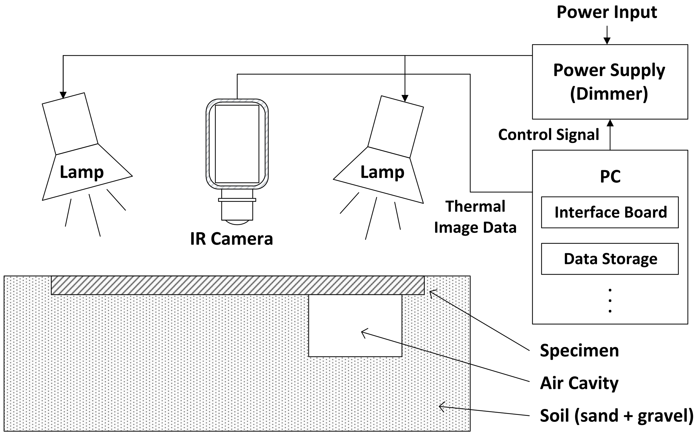
4.1. Experiment Setup and Data Acquisition

Conducting experiments with real culverts in many regions of Canada involves some challenges. Gaining access to culverts is either difficult or impossible for most part of the year due to the flow of large volumes of water and icing conditions. Moreover, only culverts whose structure contains at least one cavity with known size and location are useful for the experimental phase of the project; this information is essential for both development and performance evaluation. These kinds of records are often infrequent and accessing them requires obtaining authorization from the Ministry of Transportation. Therefore, the performance of the proposed approach is evaluated in a laboratory setup instead.
Figure 1 illustrates the experiment setup, in which a wooden box of size 78 × 33 × 60 cm 3 is used to represent the soil around the culvert pipe. The box is filled with a mixture of sand and gravel and a specimen is then placed on the top of it. Four 1000 W halogen lamps are used as the source of thermal excitation. The power of lamps is controlled through an eight-channel dimmer pack and an electronic interface circuit. With the help of this controller and adjusting the location of the lamps, we attempt to reduce the nonuniformity of thermal stimuli. Thermal images are recorded during both heating up and cooling down process using two IR cameras and a PC. The real setup is shown in Figure 2.
Thermograms are produced by a FLIR Phoenix mid-wave infrared (MWIR) camera and a Jenoptik VarioCAM long-wave infrared (LWIR) thermal camera (see Table 1 for technical specifications). Thermal cameras with cooled detectors are superior to those with uncooled detectors in terms of capture rate, spatial resolution, and thermal sensitivity; this superiority is illustrated well in [64]. Because of these advantages and the availability of the FLIR Phoenix camera in our laboratory, the analyses are made based on thermal images produced by this camera. As this is the first time, the potential of IRT for cavity detection is assessed, it is important to identify the smallest temperature differences and the FLIR Phoenix can be very useful for this purpose. A downside of the cooled models is that they are considerably more expensive. Therefore, we also use the uncooled camera to make sure about the possibility of detection with this model, which is more suitable for field work.
The experiments are conducted with two specimens (Figure 3). The first one, referred to as specimen 1, is a 2 mm flat steel plate with dimensions 70 × 30 cm 2 . To solve the low emissivity and reflection issues, it is coated with black flat paint. Since the laboratory test with this specimen cannot represent a real scenario, we carry out further experiments using specimen 2 which is a horizontal cut of a corrugated galvanized steel culvert pipe (CGSP) with a diameter of 65 cm, a thickness of 1.6 mm, and corrugations with a pitch of 68 mm and a depth of 13 mm.
To create cavities, a few different objects, as shown in Figure 4a, are used. The first air cavity is created using a 10 × 10 × 6 cm 3 cube of foam with a carved area of 6 × 6 × 3 cm 3 so that a 6 × 6 cm 2 surface of the plate is in contact with air rather than sand. The second configuration (Figure 4c,d) is almost similar to the previous one except that 1 cm of sand is located between the cavity and the lower surface of the specimen. Cavity configuration 3 (Figure 4e) is made of five different cavities: (i) cavity configuration 2; (ii) a 10 × 6 × 1.3 cm 3 foam cube with a 8 × 4 × 0.5 cm 3 hollowed area; (iii) a ping pong ball; (iv) a cylindrical ceramic ashtray with the interior radius 5.5 cm and height 2.5 cm half filled with water; and (v) a 2 × 2 × 1.5 cm 3 sponge. The last cavity of this configuration is devised to simulate the water cavity which is difficult to achieve in the laboratory setup. Using this approach allows the contact between water and the specimen through the water absorbed by the sponge. Cavity configuration 4 (Figure 4f) contains only the ashtray from the previous configuration without water.

4.2. Processing Algorithm

Figure 5 shows a summary of the processing flow. Before starting cavity detection analysis, a few preprocessing steps are required. The thermal camera, used for thermogram acquisition, records the image sequence as ‘*.sfmov’ which is based on a file format known as the Standard Archive Format (SAF). This format is not readable directly and therefore, a code snippet is developed to convert ‘*.sfmov’ files into 3D arrays (x, y, t) such that x and y represent the horizontal and vertical pixels of the thermograms, and t refers to the time slice of the recorded images. The arrays are then saved as Matlab data (‘*.mat’) files.
Raw image sequences (thermograms), representing the specimen surface temperature, are taken at 50 Hz. Recording even one minute of thermal image with the FLIR Phoenix camera can produce around 1.83 GB (640 × 512 × 2 × 50 × 60 bytes) of data. To avoid reaching the memory and computational source limits, the raw sequences are downsampled by a factor of five. We use both spatial and temporal filtering to reduce noise. The temporal filter is applied prior to downsampling to reduce the subsampling error. Then a 3 × 3 median filter in spatial domain is used. The Median filter is effective in eliminating sharp, sudden disruptive changes in the image intensity (aka salt-and-pepper noise), including a few damaged pixels of the camera. The raw thermal images include the box and its surroundings as well as the specimen. By removing the unnecessary areas, we reduce the time and computational cost.
To detect the cavities, we use three different methods. The first method is based on LPT [12,46] with ATC [12]. Based on our hypothesis (Section 3), we assume that the temperature decay of a sounding (normal) area should be different from those where a hollowed area is located. This can be verified by computing temperature contrast
Δ T = T d a T s a ,
where T d a is the temperature of a defective area (with cavity) and T s a is the temperature of a sound area (without cavity). The thermal images are also analyzed using PCT [50] and another statistical approach. These methods are discussed in detail in the following sections. To improve visualization, we normalize the thermal images (using mean and standard deviation) and apply the color mapping. The image processing algorithms are implemented in Matlab R2018a and Python.

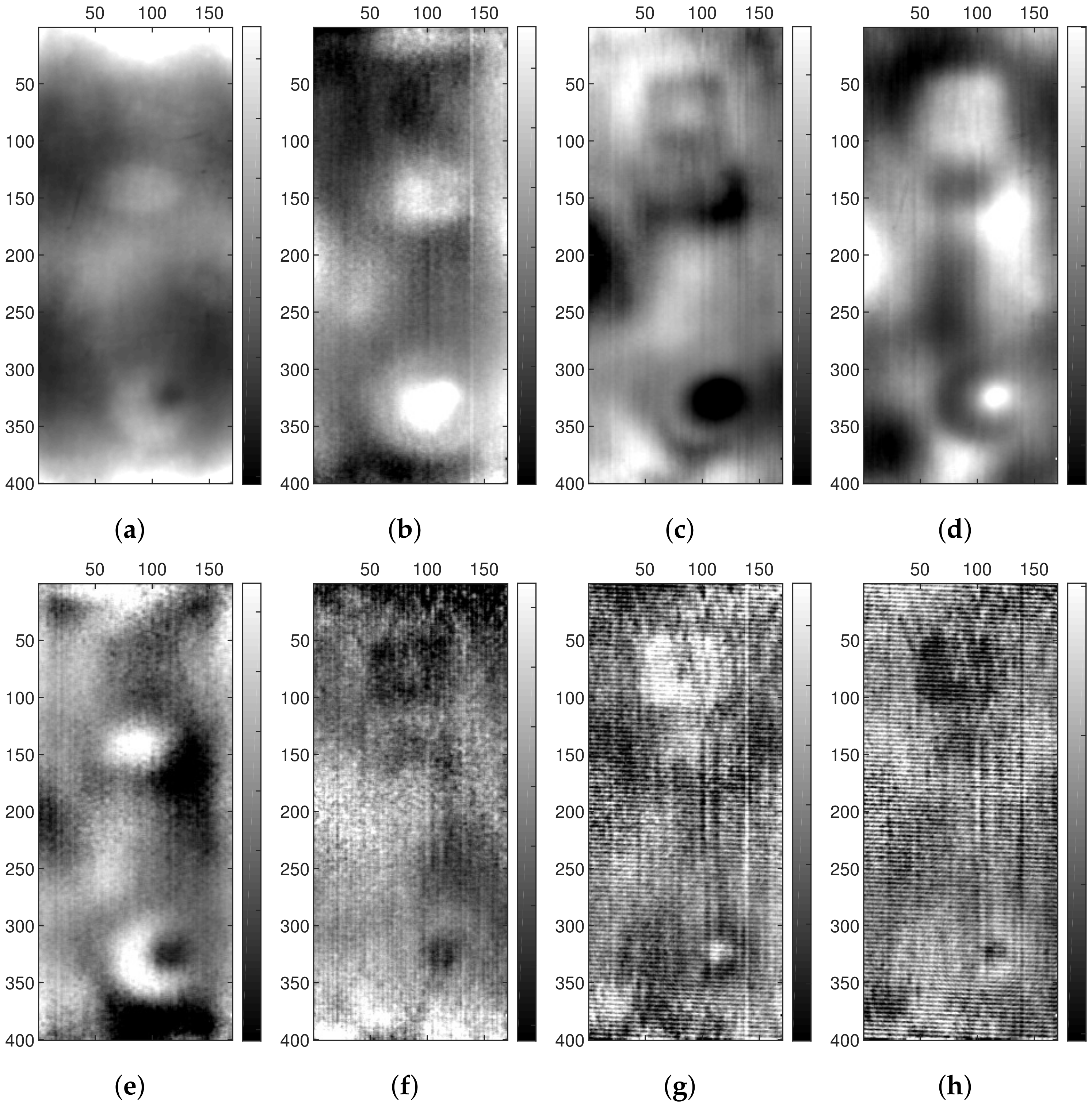
4.3. Principal Components Thermography

Principal components analysis (PCA) is a statistical approach that maps a set of possibly correlated N-dimensional data to a new space with orthogonal basis along directions with the largest variances. Data in the new space is uncorrelated (diagonal covariance matrix). In machine learning and pattern recognition, PCA is generally used to improve the curse of dimensionality and feature reduction. In some disciplines (e.g., oceanography, meteorology, and climate science) PCA is known as empirical orthogonal function (EOF) analysis [65,66]. PCT [50] is the application of PCA in thermography for nondestructive testing and inspection.
For large matrices, which is often the case in image processing, the computational cost of the traditional PCA analysis becomes extremely large and limits the usage of this approach. A more computationally effective alternative is based on singular value decomposition (SVD). In this method, similar to the traditional approach, each 2D image matrix is converted to a vector by concatenation of its row. If the thermal images are denoted by T ( i , j , k ) where i = 1 , 2 , N i , j = 1 , 2 , N k , and k = 1 , 2 , N k , then the corresponding vectors are x k = [ x 1 k , x 2 k , , x M ] T where M = N i × N j and N = N k . This process is repeated for all the images of the thermal sequence and all these column vectors are combined into a matrix as follows:
A = x 1 x 2 x N ,
in which N is the number of frames of the thermal sequence. Now, the data is normalized using its mean value and standard deviation:
A ^ ( n , m ) = A ( n , m ) μ m σ m ,
with
μ m = 1 N n = 1 N A ( m , n ) ,
σ m 2 = 1 N 1 n = 1 N A ( m , n ) μ m 2 .
Then the following factorization (known as SVD) of A ^ is used:
A ^ = U D V T ,
where U is an M × M unitary matrix (aka the left-singular vectors of A ^ ), D is a diagonal matrix consisting of singular values of A ^ , and V is an N × N unitary matrix (aka the right-singular vectors of A ^ ). Columns of U are orthonormal eigenvectors of A ^ A ^ T and singular values of A ^ are the square root of eigenvalues of A ^ A ^ T . Columns of U can be seen as basis vectors (principal components) of A ^ and their contribution to reconstruction of A ^ is determined by corresponding singular values. Singular vectors and corresponding singular values are often sorted in a descending order. The first few components contribute to more than 99% of the total data variation. Therefore, only this part of the data is used for analysis. The first few columns can be converted back to 2D matrices and shown as images that are sometimes referred to as EOFs.

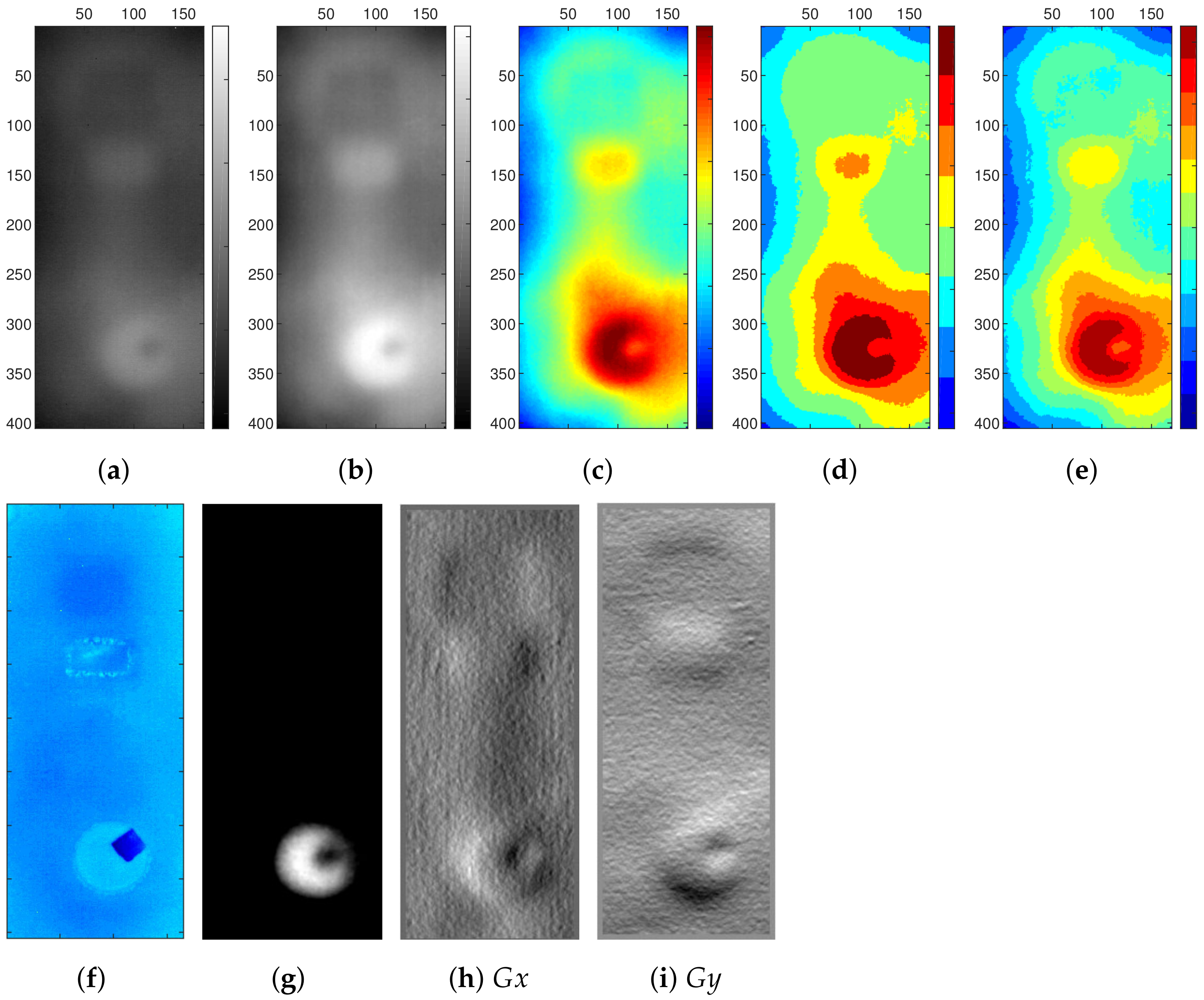
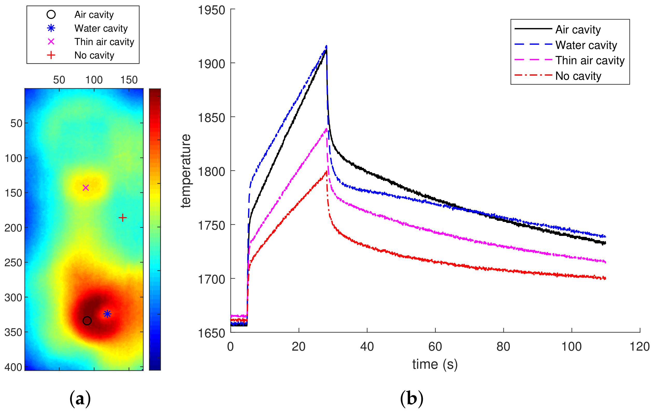
4.4. A Statistical Method for Cavity Identification

In this section, we describe a statistical approach allowing the detection of cavities in a thermal image sequence. Based on the theory described in the previous sections and using the cavity properties, we can conclude that a cavity can be identified by performing an analysis of abnormal fluctuations in temperature flow. At each frame (or time), we define an abnormal fluctuation as a temperature that is sufficiently lower or higher than the average. This assumption is made because under normal condition (no defects or cavities) the temperatures of different points on the specimen surface are very close. There are some variations due to noise, inhomogeneity of the reflections, and the impact of surface features, but these variations are usually negligible in comparison with those caused by a defect. From a statistical point of view, abnormal temperatures can be expressed as
T a b = { T | T μ c 1 σ T μ + c 1 σ } ,
where μ and σ are mean and standard deviation of the image and c 1 is a constant coefficient. An analysis of the temperature distribution at a given time allows the image pixels to be classified into normal (0) or abnormal (1) classes. However, this approach is not sufficient to determine whether a pixel actually represents a cavity, as measurements are made at each individual moment. To account for all times (or frames), we use the idea of frequentist probability. This method allows the frequency probability of an event to be inferred using a large test set, considering each thermal image as a test. Now, we assign a probabilistic measure, indicating the likelihood of being a defect, to each pixel with the following expression
P ( x , y ) = n 1 ( x , y ) n t , f o r n t 1
in which P ( x , y ) is the probability of a pixel ( x , y ) being a defect, n 1 ( x , y ) is the number of times that pixel ( x , y ) is classified as the defect category, and n t is the total number of images in the given sequence. A limit of this equation is that it treats all temperatures larger than μ + c 1 σ or smaller than μ c 1 σ similarly. However, in some cases we may need to look for temperatures within a range; similar to the idea of band pass filtering. This can be obtained by introducing terms n 2 ( x , y ) and p e n into the equation
P ( x , y ) = n 1 ( x , y ) n 2 ( x , y ) p e n n t , for n t 1
where n 2 ( x , y ) is defined like n 1 ( x , y ) , except that c 1 is replaced with c 2 , and p e n is a penalty factor from 0 to 1. When the penalty factor is 0, the expression is reduced to Equation (12). The main steps of this approach are given in Algorithm 1. With the help of coefficients c 1 and c 2 which are determined empirically, the equation can be adjusted for each experiment.
Algorithm 1 The proposed statistical algorithm for cavity detection.
Applsci 11 04051 i001

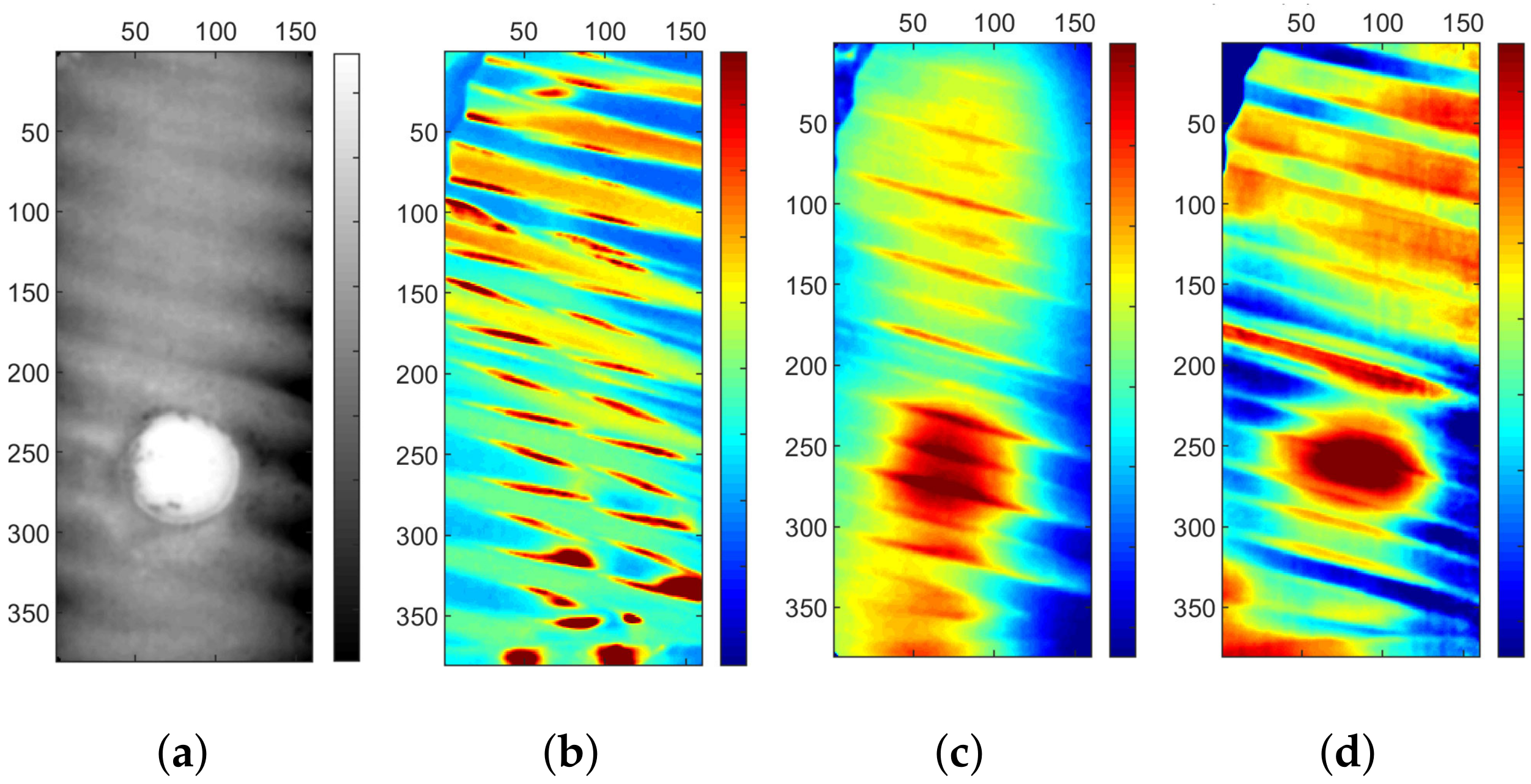
5. Experimental Results

5.1. Experiment 1: Specimen 1, Cavity Configuration 1

Raw thermal images (Figure 6a) were corrupted with noise and could not provide any clear sign of the presence of a cavity. Pre- and post-processing, as shown in Figure 6b–f, noticeably contributed to a better understanding and easier analysis of thermograms. Color mapping was also helpful and carried out at different levels of granularity to achieve a desirable output.
As mentioned before, we hypothesize that the existence of a cavity behind the specimen leads to variations in thermal radiation from the specimen surface. Although the presence of a cavity is evident in the processed thermograms (orange/yellow patch at the bottom of Figure 6c–f), further investigation was made through ATC which is a quantitative approach. Figure 7 shows the temperature-time graph for two randomly selected points, one from the sound areas (without any cavity, referred to as “sa”) and the other from the defective areas (with cavity, referred to as “da”). From this graph, it is apparent that during the transition phase (cooling down), the temperature of defective regions (red curve) cools down slower than nondefective areas (black curve). The blue curve which is the thermal contrast between the two temperatures clearly shows this.
Thermograms were also analyzed using PCT (Figure 8), and the most informative output was EOF 3. After studying the effect of filtering and other parameters of the experiment setup on the final result, we noticed that the thermal images recorded during the cooling down period, rather than the entire sequence, should be used as input to the PCT algorithm to obtain more informative results. A deeper look at the temperature graph (Figure 7) revels the underlying cause. At heap up, drastic changes occur in temperature of both sound and defective areas. As PCT is a method of obtaining major variables, it also extracts the variations of temperature in thermal excitation phase, and this makes the process of cavity identification more difficult because of blending ineffectual information to EOFs. Despite the useful role of the temporal filtering at ATC analysis, it did not perform very well for PCT. For each setup, we repeated the experiment with four different durations of the thermal stimulation. The best result was achieved when the duration was around five seconds.

5.2. Experiment 2: Specimen 1, Cavity Configuration 3

In this experiment, we combined different cavity configurations, including an air cavity, a water cavity, a thin air layer cavity, and a nonadjacent (in-depth) cavity into one setup (Figure 4e). This time the analysis began with PCT to determine if this method can provide us with any clue about the cavities in a more complicated configuration. Figure 9 shows a few selected EOFs for experiment 2. Even though the signs of cavities are not as bold and clear as in experiment 1, they are still informative and all cavities, except the small ball, can be detected. However, this time checking all first 10 EOFs from different setups was required. Contrary to the previous experiment, in which EOF3-4 carried the most information about cavities, in this experiment information spread among a larger number of EOFs, including EOF8-9. Moreover, detecting the in-depth cavity required a longer thermal stimulation.
As the usefulness of pre- and post-processing was demonstrated in the previous experiment, they were also employed for experiment 2 (see Figure 10a–e). Figure 10f is related to a test without specimen while maintaining the other parameters of the setup exactly the same as in experiment 2. This is useful for performance comparison and illustrating the accuracy and quality of the cavity detection by the proposed approach. We also examined the effectiveness of other techniques, such as thresholding and gradients. Figure 10h,i shows the power of the image gradients as four different areas representing the four cavities can be easily differentiated from the rest.
For a better understanding of the influence of different types of cavities in the IRT results, the temperature graphs (Figure 11) of the relevant regions were studied. The nondefective regions have the lowest temperature value during the cooling down phase. The second lowest temperature belongs to zone 2, above cavity 2 (thin air); as indicated in Figure 4e, a zone (1–5) is assigned to each cavity (1–5). The highest values were recorded for zone 4 (thick air cavity) and zone 5 (water cavity), respectively. These results could be anticipated in advance by analyzing the thermal effusivity of the cavity materials. According to [67], the thermal effusivity of air, water, soil (avg. properties) are approximately 6, 1588, and 1067 (588 for soil sandy dry) W s / ( m 2 K ) . Since the air thermal effusivity is significantly smaller than the soil’s, air cavity allows less thermal energy exchange, and thus the specimen temperature in zone 5 cools down slower. Due to the same phenomenon during the heating up, zone 5 warms up faster as is evident from the related graph in Figure 11. The root of difference between the decay curves of zones 2 and 4 is the presence of a thicker air layer for zone 4 which acts as a stronger insulator (between the soil and the specimen), resulting in a higher temperature increase in the heating phase and a smaller decline in the cooling period in zone 4. The behavior of cavity 5 (water) is more complex. As its thermal effusivity is higher than both dry and average property soil, we expect lower temperatures for this zone in comparison to the nondefective regions which are in contact with soil. We think this inconsistency lies on two issues. First, this cavity is not made completely from water, but a soaked sponge. Although we do not know the exact thermal effusivity for a soaked sponge, it must be smaller than water. Second, the water cavity is surrounded by cavity 4 (air) which is considerably larger. Since the highest temperature increase occurs in zone 4, a large amount of heat laterally diffuses to its surroundings. The impact of the lateral heat conduction can be clearly seen in Figure 11e. As a result, the temperature of zone 5 rises to a higher level than expected. Another interesting behavior of this zone is that its temperature gradually rises above zone 4 at around 70 s. This phenomenon can be described as follows. The high thermal effusivity of water causes quick cooling of zone 5 because of the absorption of a larger amount of energy. Over the course of heating and cooling, the internal energy of cavity 4 increases owing to the heat transfer from zone 4 to cavity 4. Part of this energy is transferred to cavity 5 due to the adjacency of zones 4 and 5 and the higher temperature of zone 4. As the heat capacity of water is a few times larger than that of air and soil, it can store a higher amount of heat energy. When the temperature of the surroundings drops below the water cavity, the water role becomes reverse and starts acting as a heat source until the system reaches the thermal equilibrium. The small ball (cavity 3) could not be detected owing to its small size. Although we could detect a deep cavity (cavity 1) using methods such as PCT and gradients, the temperature curves revealed that there is a very small temperature difference between zone 1 and the normal areas. Therefore, the reliability of this approach for detection of in-depth cavities is of concern.

5.3. Experiment 3: Specimen 2, Cavity Configuration 4

The goal of this experiment was to verify the possibility of detecting air pockets behind the real specimen using PCT and ATC. In this test, we could not detect any clear indication of a cavity using either of these techniques; an example of the results is given in Figure 12b. As the figure shows, there is no clear difference between sound and defective areas because the recorded thermal images do not carry sufficient information to distinguish between areas with the cavity and the rest. After further investigation we noticed that three matters underlie this problem: low thermal emissivity, high thermal reflection, and complex surface. Specimen 2 is a cut from a corrugated pipe with a series of ridges and grooves. The presence of these folds causes nonuniform heating of the specimen surface. Specifically, the ridges receive the largest portion of heat whereas slopes receive the smallest. This causes a relatively regular nonuniformity in the thermograms recorded by the IR camera. Consequently, the expected variations in the thermal pattern of areas with a cavity, which are considerably smaller than these effects, are lost.
To handle the first two issues with the real specimen (i.e., specimen 2), its internal layer (toward the camera) was coated by flat black paint and another experiment under exactly the same conditions was carried out. Figure 12c,d and Figure 13 show the best results achieved for the LPT analysis, including PCT and ATC. Although the thermal contrast is not as significant as for experiment 1, it is still sufficient to notice the cavity as well as estimate its size, location, and even its shape.

5.4. Experiment 4: Specimen 2, Specific Configuration

In the previous section, we showed and discussed the issue with the real specimen and demonstrated how this problem can be overcome by painting the specimen surface. However, we think in a practical setup, it might be addressed by other means as well. For instance, if the temperature of the other side of the specimen is sufficiently colder than the temperature of the air inside the pipe which can be possibly true in real scenarios, the emissivity and other problems of the real specimen will not be an issue of concern. To simulate such scenarios, some ice was placed between the original specimen (without any painting) and the soil, then the thermal radiations from the specimen surface using the same thermographic camera were recorded. In this setup, no other thermal stimuli such as halogen lamps were used. The result for a sample frame is given in Figure 14. The black/blue regions in the gray/color image, inscribed in a dashed oval, represent lower temperatures and show the location which was exposed to the ice.

5.5. Result of the Statistical Approach

We evaluated the performance of the proposed statistical approach using different values of c 1 , c 2 and p e n . For experiment 3, we obtained the best detection result (Figure 15b) with c 1 = 1 , c 2 = 1.5 and p e n = 0 . Using the images from the cooling period yielded a better outcome for both experiments (2 and 3) as illustrated in Figure 15c,d. In general, we recommend keeping the penalty value at 0. However, different visualizations of the defects are available with the help of the p e n factor. When p e n = 1 , the contour of the cavity can be shown. This feature can be useful when dealing with an automated system. By choosing a penalty around 0.5, both the contour and the surface of the cavity appear in the image but with different colors. The effectiveness of this method was also examined for experiment 2 which contains multiple cavities in one image. Using the same parameters ( c 1 , c 2 , p e n ), the most pronounced temperature fluctuations (related to cavity 4) could be easily detected (Figure 15f). By using c 1 = 0.9 , c 2 = 1.1 , we could adjust it to visualize cavity 2. This selectivity feature of the algorithm is the outcome of extending Equation (12) to (13).

6. Discussion

In our tests, we observed that the thermal behavior of the real specimen was very different from that of specimen 1 because of the dissimilarity in the material and the surface appearance. Moreover, the thermal behavior of the whole system depends on several other factors such the soil components, size and type of the pipe, the depth in which the pipe has been buried, the pipe distance from the ground surface, and ambient temperature. Preparing an experimental setup taking into account all these factors, even if possible, would be too costly and time consuming. Therefore, to verify the performance of the proposed approach for cavity detection, it is necessary to carry out further tests in real setups.
Since the passive thermography approach could not provide enough information about cavities in our experiment, the active approach was used. However, in real scenarios the thermal behavior of the whole system will be largely different and therefore we think that the passive thermography might be able to provide sufficient information for cavity detection. Since the passive approach is easier and less expensive to implement, this possibility should be investigated in a real setup.
In the experiments, some unexpected thermal patterns were observed in thermograms. Following further investigation, we realized that the presence of a thin layer of air between the specimen and the soil was the main reason behind these unexpected behaviors. It occurred because in our experimental setups, the specimens were placed on the surface of the soil and in practice it was extremely difficult to level the soil surface. Even having a leveled soil was not enough since the specimen surface was not perfectly leveled. As a result, we could not completely eliminate the thin air layer. It is worth noting that thin air layers adjacent to the specimen surface can cause a noticeable variation in the thermal radiation from the specimen surface. Nevertheless, we later realized that this feature of thermography can be very helpful in detecting other problems in a culvert. Formation of thin air layers adjacent to a culvert pipe can indicate a sign of cavity creation in earlier stages, and our experiments unexpectedly show that this stage can be identified through IRT.
Before achieving the reported results, a set of parameters had to be determined. For example, the duration of thermal stimuli has a crucial impact on the quality of thermal images and may dictate the level of information that can be extracted from thermograms. Very short and weak thermal excitation may not be enough for the detection of the required information while long and strong thermal stimuli may yield more fruitful thermograms, but they extend the test period and usually are more costly. Moreover, the optimal parameters for PCT and ACT were not the same necessarily. For PCT, we obtained the best result when the length of the heating up period was about 5–10 s whereas for ACT the better results were achieved with longer thermal stimulation. Also, we noticed that the detection of deeper cavities requires longer stimulation as the heat propagation is slow, thereby taking more time to reach deeper layers. Consequently, conducting experiments with different heating periods is necessary for a successful cavity detection. In addition to the thermal stimuli, it is necessary to adjust a few other parameters such as the distance between the camera and specimen, the distance between the thermal sources and specimen, locations and directions of thermal sources (to minimize nonuniform excitation on the specimen surface). We think the results, reported in this paper, can be improved by further tuning of these parameters.
Future work should consider the limitations of the proposed approach for cavity detection. To inspect a culvert in a real setup using the proposed approach, the IR camera and halogen lamps should be placed inside the pipe. For large-span pipes (large than 2 m), this can be done in different ways, but for smaller pipes, we recommend using a small robot to navigate through the pipe while the camera and lamps are installed on it. Considering the size of the camera and lamps, and the required distance between the camera and the interior surface of the camera, the current version of the proposed approach is not suitable for pipes with a diameter smaller than 1.2 m. However, by deploying modern cameras (e.g., FLIR Boson) which are available in very small sizes, inspecting smaller pipes is practical; the size of a FLIR Boson without a lens is only 21 × 21 × 11 mm 3 . Metallic materials generally have very low emissivity, thereby reflecting thermal waves strongly. Generally speaking, IRT is not appropriate for inspection of low emissivity materials including metals, unless surface coating is allowed [12,15]. In our laboratory tests, we had to paint the specimen to deal with a very shiny surface of the specimen as it was a cut from a brand-new pipe. However, this problem will be of less importance as inspection is often carried out for old pipes whose surfaces become unpolished due to erosion, accumulation of dirt, and other factors. In the worst-case scenario, the low emissivity can be addressed by painting. In most experiments, the cavities were directly in contact with the specimen. In experiment 3, one of cavities was placed at a distance of 1 cm from the specimen and the gap was filled with the soil. Detecting this cavity was noticeably more difficult than detecting the other cavities, and we expressed our concern about the reliability of this approach for detecting deep cavities. This is consistent with the fact that the main limitation of IRT is the penetration depth. Therefore, we suggest future research to measure the maximum depth in which the detection is possible. Moreover, infrared waves cannot penetrate through water and therefore the surface areas of the culvert that are under water cannot be investigated.

7. Conclusions

This study aimed to assess the potential of IRT as a complementary (or alternative) approach to identify the presence of cavities in a certain type of culvert. Empirical studies in a laboratory setup showed the efficacy of IRT for detecting cavities even of small sizes (a few centimeters). The size and location of cavities are among the aspects that can be extracted from analyzing thermograms. In examining the real specimen, we faced some difficulties including the emissivity issue, which we could effectively deal with by coating. Although this study showed a promising future for the application of IRT in culvert inspection, further research is necessary. In particular, it is essential to verify the power of the technique in real setups despite logistic and technical difficulties of the on-site evaluation. Another direction that future research should consider is the fine tuning of the experimental setup and parameters as discussed in Section 6.

Author Contributions

D.K.: Conceptualization, Methodology, Formal Analysis, Experimental Setup and Data Acquisition, Validation, Software, Writing (original, review and editing); S.E.: Conceptualization, Simulation, Literature Review, Writing (literature review); R.B.T.: Conceptualization, Methodology (statistical method for cavity identification), Software (section statistical method for cavity identification); F.A.M.: Conceptualization, Simulation; Y.B.: Conceptualization, Theoretical Basis; A.M.: Conceptualization, Methodology (section statistical method for cavity identification), Software (section statistical method for cavity identification); X.M.: Conceptualization, Supervision, Project Administration, Resources, Funding Acquisition. All authors have read and agreed to the published version of the manuscript.

Funding

This research is funded by the Natural Sciences and Engineering Research Council of Canada (NSERC)—Discovery Grant Program, the Canadian Foundation for Innovation (CFI) and Canada Research Chair Program (MIVIM Multipolar Infrared Vision Infrarouge Multipolaire).

Institutional Review Board Statement

Not applicable.

Informed Consent Statement

Not applicable.

Data Availability Statement

Data sharing not applicable.

Acknowledgments

We would like to express our gratitude for the precious support of Richard Drouin and his colleagues from Ministère des transports du Québec. The authors are also grateful to Clemente Ibarra-Castanedo for his valuable advice during experiments and thank Denis Ouellet for his kind help with preparation for the experiment setup.

Conflicts of Interest

The authors declare no conflict of interest.

Abbreviations

The following abbreviations are used in this manuscript:
ACTAbsolute thermal contrast
APTAbsolute phase contrast
EOFEmpirical orthogonal function
LPTLong pulse thermography
LTLock-in thermography
IRTInfrared thermography
NDTnondestructive testing
PCAPrincipal components analysis
PCTPrincipal components thermography
PTPulse thermography
PPTPulsed phase thermography

References

  1. Cabonce, J.; Fernando, R.; Wang, H.; Chanson, H. Using small triangular baffles to facilitate upstream fish passage in standard box culverts. Environ. Fluid Mech. 2019, 19, 157–179. [Google Scholar] [CrossRef] [Green Version]
  2. Donaldson, B. Use of highway underpasses by large mammals and other wildlife in Virginia: Factors influencing their effectiveness. Transp. Res. Rec. 2007, 2011, 157–164. [Google Scholar] [CrossRef]
  3. TRB. Culverts and Soil–Structure Interaction: Fifty Years of Change and A Twenty-Year Projection; Technical Report E-C230; Transportation Research Board: Washington, DC, USA, 2018. [Google Scholar]
  4. Sheth, A.; Sinfield, J.V. Synthesis Study: Overview of Readily Available Culvert Inspection Technologies (Joint Transportation Research Program); Technical Report FHWA/IN/JTRP-2018/17; Lyles School of Civil Engineering, Purdue University: West Lafayette, IN, USA, 2018. [Google Scholar]
  5. Piratla, K.R.; Pang, W.; Jin, H.; Stoner, M. Best Practices for Assessing Culvert Health and Determining Appropriate Rehabilitation Methods: A Research Project in Support of Operational Requirements for the South Carolina Department of Transportation; Technical Report; South Carolina Department of Transportation, Office of Materials and Research: Clemson, SC, USA, 2016.
  6. Atef, A.; Zayed, T.; Hawari, A.; Khader, M.; Moselhi, O. Multi-tier method using infrared photography and GPR to detect and locate water leaks. Autom. Constr. 2016, 61, 162–170. [Google Scholar] [CrossRef]
  7. Stampolidis, A.; Soupios, P.; Vallianatos, F.; Tsokas, G. Detection of leaks in buried plastic water distribution pipes in urban places-a case study. In Proceedings of the 2nd International Workshop on Advanced Ground Penetrating Radar, Delft, The Netherlands, 14–16 May 2003; pp. 120–124. [Google Scholar]
  8. Thitimakorn, T.; Kampananon, N.; Jongjaiwanichkit, N.; Kupongsak, S. Subsurface void detection under the road surface using ground penetrating radar (GPR), a case study in the Bangkok metropolitan area, Thailand. Int. J. Geo-Eng. 2016, 7, 1–9. [Google Scholar] [CrossRef] [Green Version]
  9. Chen, D.H.; Wimsatt, A. Inspection and Condition Assessment Using Ground Penetrating Radar. J. Geotech. Geoenviron. Eng. 2010, 136, 207–214. [Google Scholar] [CrossRef]
  10. Lefebvre, G.; Karray, M. New developments in in-situ characterization using Rayleigh waves. In Proceedings of the 51st Canadian Geotechnical Conference, Edmonton, AB, Canada, 4–7 October 1998; pp. 821–828. [Google Scholar]
  11. Karray, M.; Lefebvre, G. Détection des cavités sous les pavages par l’analyse modal des ondes de Rayleigh (MASW). Can. Geotech. J. 2009, 46, 424–437. [Google Scholar] [CrossRef]
  12. Maldague, X. Theory and Practice of Infrared Technology for Nondestructive Testing; John Wiley & Sons: New York, NY, USA, 2001. [Google Scholar]
  13. Meola, C.; Carlomagno, G.M.; Giorleo, L. The use of infrared thermography for materials characterization. J. Mater. Process. Technol. 2004, 155–156, 1132–1137. [Google Scholar] [CrossRef]
  14. Ibarra-Castanedo, C.; Maldague, X. Pulsed phase thermography reviewed. Quant. Infrared Thermogr. J. 2004, 1, 47–70. [Google Scholar] [CrossRef]
  15. Ibarra-Castanedo, C.; Tarpani, J.R.; Maldague, X.P.V. Nondestructive testing with thermography. Eur. J. Phys. 2013, 34, S91–S109. [Google Scholar] [CrossRef]
  16. Qu, Z.; Jiang, P.; Zhang, W. Development and Application of Infrared Thermography Non-Destructive Testing Techniques. Sensors 2020, 20, 3851. [Google Scholar] [CrossRef]
  17. Maillard, S.; Cadith, J.; Bouteille, P.; Legros, G.; Bodnar, J.; Detalle, V. Non-destructive testing of forged metallic materials by active infrared thermography. Int. J. Thermophys. 2012, 33, 1982–1988. [Google Scholar] [CrossRef]
  18. Chaki, S.; Marical, P.; Panier, S.; Bourse, G.; Mouftiez, A. Interfacial defects detection in plasma-sprayed ceramic coating components using two stimulated infrared thermography techniques. NDT E Int. 2011, 44, 519–522. [Google Scholar] [CrossRef]
  19. Almond, D.P.; Peng, W. Thermal imaging of composites. J. Microsc. 2001, 201, 163–170. [Google Scholar] [CrossRef] [PubMed] [Green Version]
  20. Ibarra-Castanedo, C.; Piau, J.M.; Guilbert, S.; Avdelidis, N.P.; Genest, M.; Bendada, A.; Maldague, X.P.V. Comparative Study of Active Thermography Techniques for the Nondestructive Evaluation of Honeycomb Structures. Res. Nondestruct. Eval. 2009, 20, 1–31. [Google Scholar] [CrossRef]
  21. Sakagami, T.; Kubo, S. Development of a new non-destructive testing technique for quantitative evaluations of delamination defects in concrete structures based on phase delay measurement using lock-in thermography. Infrared Phys. Technol. 2002, 43, 311–316. [Google Scholar] [CrossRef]
  22. Bison, P.; Marinetti, S.; Cuogo, G.; Molinas, B.; Zonta, P.; Grinzato, E. Corrosion detection on pipelines by IR thermography. In Thermosense: Thermal Infrared Applications XXXIII; International Society for Optics and Photonics: Bellingham, WA, USA, 2011; Volume 8013, pp. 116–125. [Google Scholar]
  23. Rodríguez-Martin, M.; Lagüela, S.; González-Aguilera, D.; Arias, P. Cooling analysis of welded materials for crack detection using infrared thermography. Infrared Phys. Technol. 2014, 67, 547–554. [Google Scholar] [CrossRef]
  24. Milovanović, B.; Banjad Pečur, I. Review of active IR thermography for detection and characterization of defects in reinforced concrete. J. Imaging 2016, 2, 11. [Google Scholar] [CrossRef]
  25. Yang, J.; Wang, W.; Lin, G.; Li, Q.; Sun, Y.; Sun, Y. Infrared Thermal Imaging-Based Crack Detection Using Deep Learning. IEEE Access 2019, 7, 182060–182077. [Google Scholar] [CrossRef]
  26. Costello, S.; Chapman, D.; Rogers, C.; Metje, N. Underground asset location and condition assessment technologies. Tunn. Undergr. Space Technol. 2007, 22, 524–542. [Google Scholar] [CrossRef]
  27. Yang, C.; Allouche, E. Evaluation of non-destructive methods for condition assessment of culverts and their embedment. In Proceedings of the ICPTT 2009: Advances and Experiences with Pipelines and Trenchless Technology for Water, Sewer, Gas, and Oil Applications, Shanghai, China, 18–21 October 2009; pp. 28–38. [Google Scholar]
  28. Meola, C. Infrared Thermography Recent Advances and Future Trends; Bentham Science Publishers: New York, NY, USA, 2012. [Google Scholar]
  29. Osornio-Rios, R.A.; Antonino-Daviu, J.A.; de Jesus Romero-Troncoso, R. Recent industrial applications of infrared thermography: A review. IEEE Trans. Ind. Inform. 2018, 15, 615–625. [Google Scholar] [CrossRef]
  30. Ciampa, F.; Mahmoodi, P.; Pinto, F.; Meo, M. Recent advances in active infrared thermography for non-destructive testing of aerospace components. Sensors 2018, 18, 609. [Google Scholar] [CrossRef] [PubMed] [Green Version]
  31. Breitenstein, O.; Warta, W.; Schubert, M.C. Lock-in Thermography: Basics and Use for Evaluating Electronic Devices and Materials; Springer: Berlin, Germany, 2019; Volume 10. [Google Scholar]
  32. Giorleo, G.; Meola, C. Comparison between pulsed and modulated thermography in glass–epoxy laminates. Ndt E Int. 2002, 35, 287–292. [Google Scholar] [CrossRef]
  33. Dillenz, A.; Zweschper, T.; Riegert, G.; Busse, G. Progress in phase angle thermography. Rev. Sci. Instrum. 2003, 74, 417–419. [Google Scholar] [CrossRef]
  34. BuSSe, G.; Wu, D.; Karpen, W. Thermal wave imaging with phase sensitive modulated thermography. J. Appl. Phys. 1992, 71, 3962–3965. [Google Scholar] [CrossRef]
  35. Ibarra-Castanedo, C. Quantitative Subsurface Defect Evaluation by Pulsed Phase Thermography: Depth Retrieval with the Phase. Ph.D. Thesis, Laval University, Quebec, QC, Canada, 2005. [Google Scholar]
  36. Carlomagno, G.M.; Meola, C. Comparison between thermographic techniques for frescoes NDT. NDT E Int. 2002, 35, 559–565. [Google Scholar] [CrossRef]
  37. Gleiter, A.; Spiessberger, C.; Busse, G. Lockin thermography with optical or ultrasound excitation. Stroj. Vestn. J. Mech. Eng. 2010, 56, 619–624. [Google Scholar]
  38. Jia, Y.; Tang, L.; Ming, P.; Xie, Y. Ultrasound-excited thermography for detecting microcracks in concrete materials. NDT E Int. 2019, 101, 62–71. [Google Scholar] [CrossRef]
  39. Dong, W.; Wu, Z.; Zhou, X.; Tan, Y. Experimental studies on void detection in concrete-filled steel tubes using ultrasound. Constr. Build. Mater. 2016, 128, 154–162. [Google Scholar] [CrossRef] [Green Version]
  40. Lin, S.; Shams, S.; Choi, H.; Azari, H. Ultrasonic imaging of multi-layer concrete structures. NDT E Int. 2018, 98, 101–109. [Google Scholar] [CrossRef]
  41. Sophian, A.; Tian, G.; Fan, M. Pulsed eddy current non-destructive testing and evaluation: A review. Chin. J. Mech. Eng. 2017, 30, 500–514. [Google Scholar] [CrossRef] [Green Version]
  42. Xu, X.; Ji, H.; Qiu, J.; Takagi, T. Detection of delamination in laminated CFRP composites using eddy current testing: Simulation and experimental study. Int. J. Appl. Electromagn. Mech. 2018, 57, 177–192. [Google Scholar] [CrossRef]
  43. Yin, A.; Gao, B.; Yun Tian, G.; Woo, W.L.; Li, K. Physical interpretation and separation of eddy current pulsed thermography. J. Appl. Phys. 2013, 113, 064101. [Google Scholar] [CrossRef]
  44. Wang, Z.; Zhu, J.; Tian, G.; Ciampa, F. Comparative analysis of eddy current pulsed thermography and long pulse thermography for damage detection in metals and composites. NDT E Int. 2019, 107, 102155. [Google Scholar] [CrossRef]
  45. Lau, S.; Almond, D.; Patel, P. Transient thermal wave techniques for the evaluation of surface coatings. J. Phys. D Appl. Phys. 1991, 24, 428. [Google Scholar] [CrossRef]
  46. Almond, D.P.; Angioni, S.L.; Pickering, S.G. Long pulse excitation thermographic non-destructive evaluation. NDT E Int. 2017, 87, 7–14. [Google Scholar] [CrossRef] [Green Version]
  47. Kalyanavalli, V.; Ramadhas, T.A.; Sastikumar, D. Long pulse thermography investigations of basalt fiber reinforced composite. NDT E Int. 2018, 100, 84–91. [Google Scholar] [CrossRef]
  48. Krapez, J.C.; Cielo, P. Thermographic nondestructive evaluation: Data inversion procedures Part I: 1-D analysis. Res. Nondestruct. Eval. 1991, 3, 81–100. [Google Scholar] [CrossRef]
  49. Maldague, X.; Marinetti, S. Pulse phase infrared thermography. J. Appl. Phys. 1996, 79, 2694–2698. [Google Scholar] [CrossRef]
  50. Rajic, N. Principal component thermography for flaw contrast enhancement and flaw depth characterisation in composite structures. Compos. Struct. 2002, 58, 521–528. [Google Scholar] [CrossRef]
  51. Gonzalez, R.C.; Woods, R.E. Digital Image Processing, 3rd ed.; Pearson: London, UK, 2008. [Google Scholar]
  52. Krapez, J.C.; Maldague, X.; Cielo, P. Thermographic nondestructive evaluation: Data inversion procedures Part II: 2-D analysis and experimental results. Res. Nondestruct. Eval. 1991, 3, 101–124. [Google Scholar] [CrossRef]
  53. Avdelidis, N.; Almond, D.P. Through skin sensing assessment of aircraft structures using pulsed thermography. NDT E Int. 2004, 37, 353–359. [Google Scholar] [CrossRef]
  54. González, D.; Ibarra-Castanedo, C.; Pilla, M.; Klein, M.; López-Higuera, J.; Maldague, X. Automatic interpolated differentiated absolute contrast algorithm for the analysis of pulsed thermographic sequence. In Proceedings of the 7th Conference on Quantitative InfraRed Thermography (QIRT), Rhode Saint Genèse, Belgium, 5–8 July 2004; pp. 1–6. [Google Scholar]
  55. Benítez, H.D.; Ibarra-Castanedo, C.; Bendada, A.; Maldague, X.; Loaiza, H.; Caicedo, E. Definition of a new thermal contrast and pulse correction for defect quantification in pulsed thermography. Infrared Phys. Technol. 2008, 51, 160–167. [Google Scholar] [CrossRef]
  56. Bai, W.; Wong, B. Evaluation of defects in composite plates under convective environments using lock-in thermography. Meas. Sci. Technol. 2001, 12, 142. [Google Scholar] [CrossRef]
  57. Jolliffe, I.T.; Cadima, J. Principal component analysis: A review and recent developments. Philos. Trans. R. Soc. A Math. Eng. Sci. 2016, 374, 20150202. [Google Scholar] [CrossRef]
  58. Milovanović, B.; Gaši, M.; Gumbarević, S. Principal Component Thermography for Defect Detection in Concrete. Sensors 2020, 20, 3891. [Google Scholar] [CrossRef]
  59. Gauci, J.; Camilleri, K.P.; Falzon, O. Principal component analysis for dynamic thermal video analysis. Infrared Phys. Technol. 2020, 109, 103359. [Google Scholar] [CrossRef]
  60. Winfree, W.P.; Cramer, K.E.; Zalameda, J.N.; Howell, P.A.; Burke, E.R. Principal component analysis of thermographic data. In Thermosense: Thermal Infrared Applications XXXVII; International Society for Optics and Photonics: Bellingham, WA, USA, 2015; Volume 9485, pp. 211–221. [Google Scholar]
  61. Liang, T.; Ren, W.; Tian, G.Y.; Elradi, M.; Gao, Y. Low energy impact damage detection in CFRP using eddy current pulsed thermography. Compos. Struct. 2016, 143, 352–361. [Google Scholar] [CrossRef] [Green Version]
  62. D’Accardi, E.; Palumbo, D.; Tamborrino, R.; Galietti, U. Quantitative analysis of thermographic data through different algorithms. Procedia Struct. Integr. 2018, 8, 354–367. [Google Scholar] [CrossRef]
  63. Carslaw, H.S.; Jaeger, J.C. Conduction of Heat in Solids; Number BOOK; Clarendon Press: Oxford, UK, 1992. [Google Scholar]
  64. Flir. Cooled or Uncooled? Available online: https://www.flir.ca/discover/rd-science/cooled-or-uncooled/ (accessed on 31 March 2021).
  65. Zhang, Z.; Moore, J.C. Chapter 6—Empirical Orthogonal Functions. In Mathematical and Physical Fundamentals of Climate Change; Elsevier: Boston, MA, USA, 2015; pp. 161–197. [Google Scholar]
  66. Thomson, R.E.; Emery, W.J. Data Analysis Methods in Physical Oceanography, 3rd ed.; Elsevier: Boston, MA, USA, 2014. [Google Scholar]
  67. Thermtest. Materials Thermal Properties Database. Available online: https://thermtest.com/materials-database (accessed on 8 April 2021).
Figure 1. The experiment setup overview.
Applsci 11 04051 g001
Figure 2. The real experiment setup. (a) Halogen Lamp, (b) IR Camera 1 (FLIR Phoenix), (c) IR Camera 2 (Jenoptik VarioCAM), (d) Specimen, (e) Box (filled with sand and gravel), (f) PC.
Applsci 11 04051 g002
Figure 3. Specimens used in tests. (a) Specimen 1. (b) Specimen 2.
Applsci 11 04051 g003
Figure 4. Cavity configurations used in tests. (a) Objects used to create cavities. (b) Cavity configuration 1. (c) Cavity configuration 2 (within the process). (d) Cavity configuration 2 (cannot be seen since it is covered by soil). (e) Cavity configuration 3 (combined 5 different cavities in one setup). (f) Cavity configuration 4.
Applsci 11 04051 g004
Figure 5. Processing flow. ATC: Absolute Thermal Contrast, PCT: Principal Components Thermography.
Applsci 11 04051 g005
Figure 6. Impact of pre- and post-processing on image quality; experiment 1. (a) An example of the raw image. (b) The processed image. (cf) Color mapping (64, 10, 5, and 3 levels).
Applsci 11 04051 g006
Figure 7. ATC; experiment 1. (a) Selected points. (b) Temperature-time graph and thermal contrast.
Applsci 11 04051 g007
Figure 8. PCT analysis (EOF3); experiment 1. (a) Setup 1 (best result). The cavity is located exactly under the blue square patch at the bottom of image. (b) Setup 2. (c) Setup 3. (d) Setup 4. Input: cooling down frames for Setup 1, 3, 4 and the entire image sequence for Setup 2. Heating up period: 5 s for Setup 1–3 and 25 s for Setup 4. Temporal filtering was applied only in setup 3.
Applsci 11 04051 g008
Figure 9. PCT analysis; experiment 2. (a) EOF2. (b) EOF3. (c) EOF3. (d) EOF3. (e) EOF4. (f) EOF7. (g) EOF8. (h) EOF9. Heating up period for (ah): 10, 10, 25, 40, 10, 25, and 40 s, respectively.
Applsci 11 04051 g009
Figure 10. LPT analysis; experiment 2. (a) An example of the raw image. (be) After pre- and post-processing. (f) A sample thermogram for experiment 2 without any specimen for cavity configuration 3. (g) Thresholding. (h,i) Gradient of the image along the x and y direction: G x = I ( x , y ) x and G y = I ( x , y ) y .
Applsci 11 04051 g010
Figure 11. Temperature comparison; experiment 2. (a) Selected points. (b) Temperature-time graph for non-cavity regions vs. different cavities.
Applsci 11 04051 g011
Figure 12. LPT analysis; Experiment 3. (a) LPT with no specimen. (b) LPT with original specimen 2. (c) LPT with painted (flat) specimen 2. (d) PCT for painted (flat) specimen 2. The same cavity configuration was used for (ad).
Applsci 11 04051 g012
Figure 13. ATC; Experiment 3. (a) Selected points. (b) Temperature-time graph and thermal contrast.
Applsci 11 04051 g013
Figure 14. IRT with cold stimuli; experiment 4. Blue regions inside the dashed oval show the effect of a cold stimulus behind the specimen. (a) The processed image. (b) Color mapping.
Applsci 11 04051 g014
Figure 15. Probability map. (ad) Experiment 3. (eh) Experiment 2. (a,e) Computed using all frames. (bd,fh) Computed using frames of the cooling down phase. All results, except the one shown in (h), were obtained with the same c 1 and c 2 ; see the text for the details. p e n : the penalty factor.
Applsci 11 04051 g015
Table 1. Thermal camera specifications.
FeatureFLIR PhoenixJenoptik VarioCAM
IR detectorCooled Indium Antimonide (InSb)Uncooled microbolometer array (FPA)
Image resolution640 × 512640 × 480
Spectral range3–5 m7.5–14 m
Thermal sensitivity<25 mK<70 mK; <30 mK at 30  C object
Frame rate50 Hz50 Hz (PAL), 60 Hz (NTSC)
Publisher’s Note: MDPI stays neutral with regard to jurisdictional claims in published maps and institutional affiliations.

