
A Shader-Based Ray Tracing Engine


1
KOG Inc., Daegu 41937, Korea
2
School of Computer Science and Engineering, Kyungpook National University, Daegu 41566, Korea
3
Department of Data Convergence Computing, Kyungpook National University, Daegu 41566, Korea
4
Dassomey.com Inc., Daegu 41566, Korea
*
Author to whom correspondence should be addressed.
Appl. Sci. 2021, 11(7), 3264; https://doi.org/10.3390/app11073264
Submission received: 13 February 2021
/
Revised: 28 March 2021
/
Accepted: 30 March 2021
/
Published: 6 April 2021
(This article belongs to the Collection Big Data Analysis and Visualization Ⅱ)
Abstract
:Recently, ray tracing techniques have been highly adopted to produce high quality images and animations. In this paper, we present our design and implementation of a real-time ray-traced rendering engine. We achieved real-time capability for triangle primitives, based on the ray tracing techniques on GPGPU (general-purpose graphics processing unit) compute shaders. To accelerate the ray tracing engine, we used a set of acceleration techniques, including bounding volume hierarchy, its roped representation, joint up-sampling, and bilateral filtering. Our current implementation shows remarkable speed-ups, with acceptable error values. Experimental results shows 2.5–13.6 times acceleration, and less than 3% error values for the 95% confidence range. Our next step will be enhancing bilateral filter behaviors.
1. Introduction
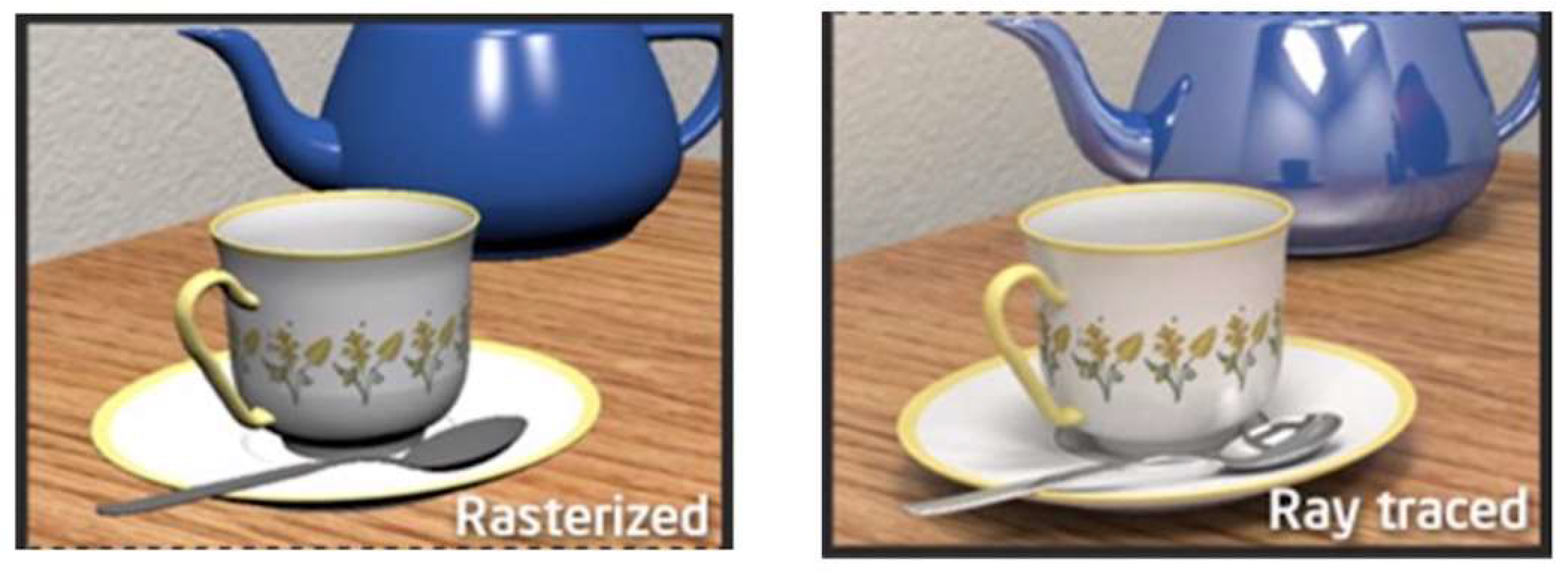
The usefulness of computer graphics in various fields has long been emphasized since its origin [1,2]. Ray tracing is a graphics method, based on the individual optical path tracing to get realistic illustrations, as shown in Figure 1. More precisely, this method traces millions of rays (or optical paths), which are intersecting, scattering, and reflecting on object surfaces, with a huge amount of computations [3,4]. Mainly due to its computation cost, it is considered as nearly impossible to carry it out on run time [5,6].
With the need for the immediate visualization, graphics processors were demanded to be specialized in the traditional rasterization technique, consuming conspicuously lower resources than the ray tracing in the cost of low precision [7,8].
In contrast, rasterization cannot compute optical phenomena such as scattering and/or reflection, resulting in comparatively unrealistic illumination as a result. Research has been made to overcome this drawbacks, introducing novel ideas such as image-based lighting, irradiance probe, pre-processed global illumination, and more [9,10,11]. More recently, hybrid methods using both rasterization and ray tracing technique have been introduced to qualify the demands for truthful illumination and is still an ongoing topic; screen-space global illumination, voxel-based global illumination, and photon mapping are a few of them [12,13,14,15,16].
In this paper, we present our research and implementation of the real-time ray-traced rendering engine, tackling the previously known to be bound to the pre-rendering domain. We introduce the real-time implementation of a triangle primitive, based the ray tracing method on the top of the GPGPU compute shader, along with optimization and light approximation techniques. We also present the solutions to the detailed issues, which we encountered during its design and implementation.
2. Related Works
In computer graphics field, interactive realistic graphics results have long been pursued [17,18]. Ray tracing is one of them, but it has only recently been applied and commercialized due to its immense computing cost in real-time. Since it considers global illumination environment, rather than the traditional local illumination settings, the ray tracing is one of the global illumination and/or indirect illumination methods [6,19]. It enables the rendering pipeline to achieve more realistic graphics rendering, as shown in Figure 1.
Ray tracing is actually rendering an image by recursively tracing optical paths from the viewer’s eye to virtual light sources per pixel [5]. It considers reflection, refraction, and scattering to ultimately compose the luminosity upon the ray’s surface contact [20]. From its accelerated implementation point of view, we should consider two different aspects: global object management for the efficient ray-object intersection checks, and accelerated reflection computing at the intersection points.
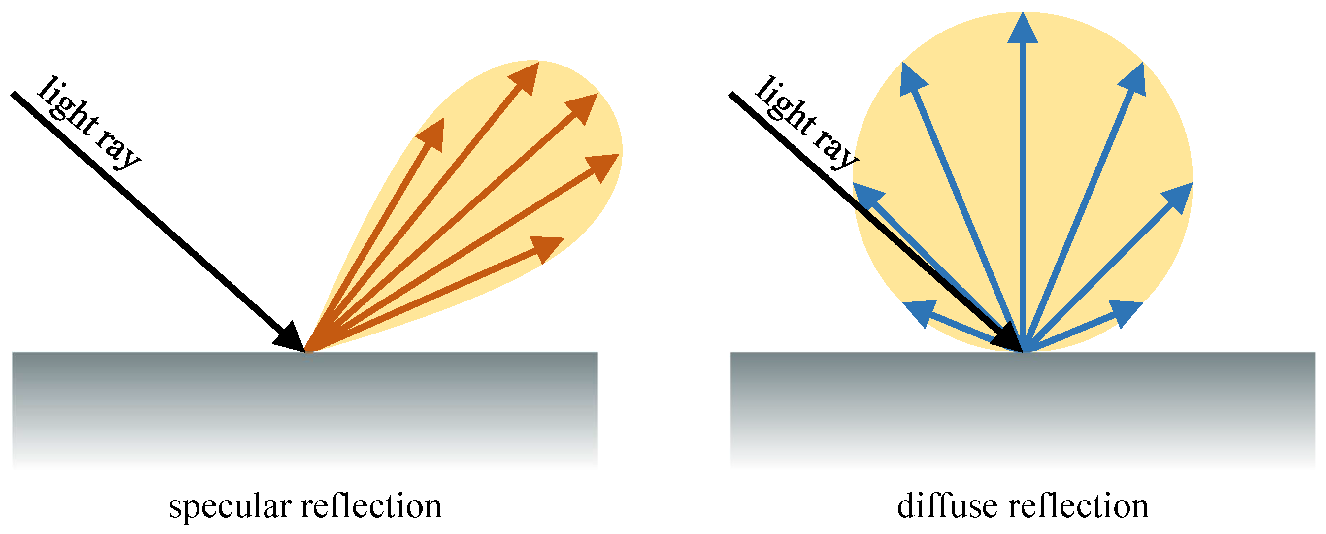
Reflection computing is again macroscopically divided into two parts: specular and diffuse. The specular reflection is a regular reflection on a mirror-like surface, and the diffuse reflection is a light scattering occurred on a rough surface, as shown in Figure 2.
Theoretically, the rays can be traced infinitely, to get the huge number of reflected bounces. In contrast, practical implementations limits the reflection computing to get real-time results. The two major factors of the real-time reflection computing is: ray bouncing count and ray sampling count. These factors are also related to the final quality of the ray traced rendering images [6,20].
Specular reflection is highly associated with the ray bouncing count, which refers to how much will the single ray bounce between the object surfaces. Likewise, diffuse reflection is associated with the ray sampling count referring to how many rays will be fired on the reflection points. The sampling attribute also affects the anti-aliasing quality of the image, since it is actually one of the super-sampling methods.
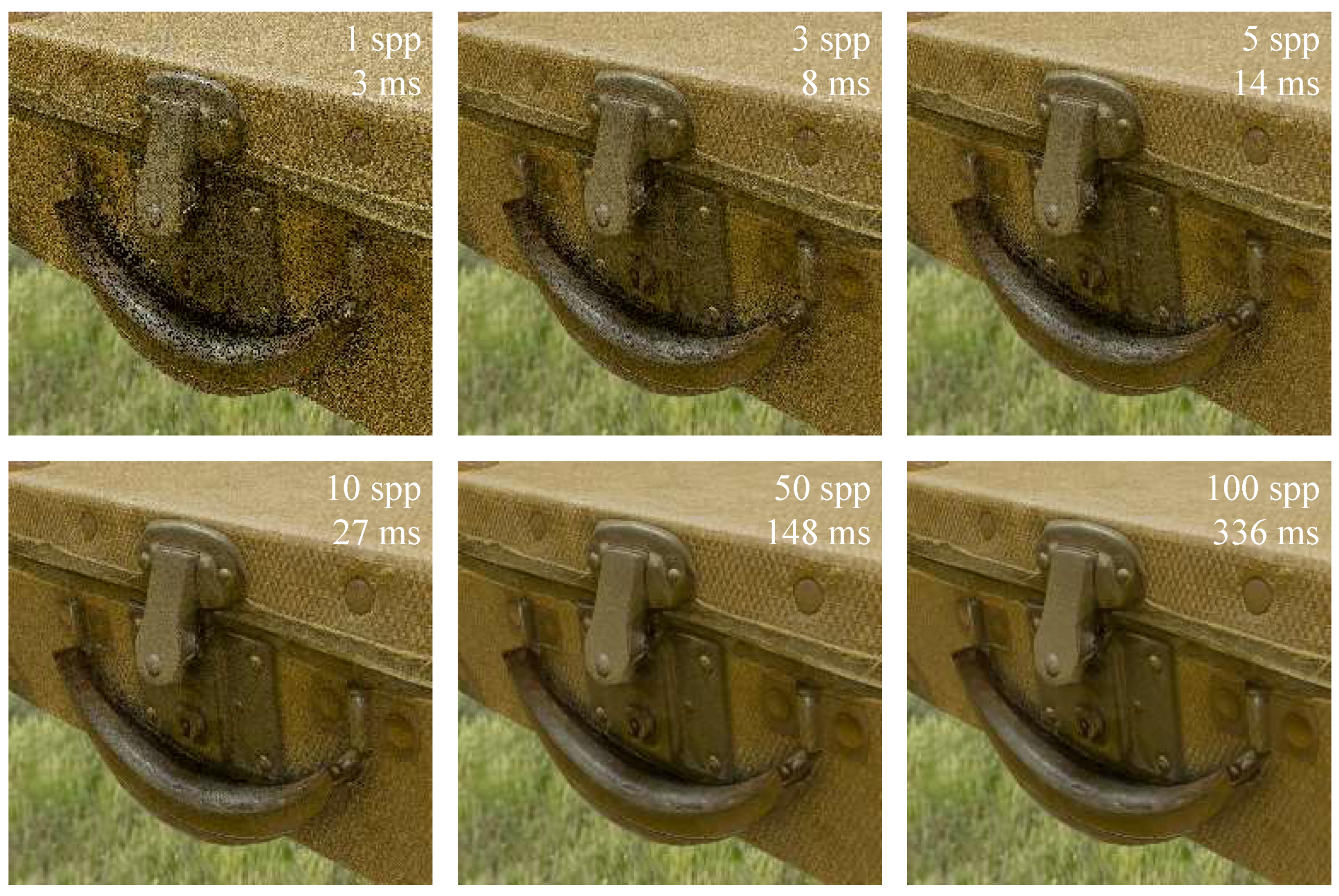
The ray bouncing is known to be significantly cost-effective than the ray sampling since it occurs seldom in the actual rendering environment; five to six bounces is more than enough in most rendering cases. Ray sampling, on the other hand, is the major reason why ray tracing lacks performance in real-time rendering all the time; due to its nature of omni-directional light scattering, not enough ray sampling will produce disturbingly noisy illumination as a result. Figure 3 depicts the performance and precision of the implemented diffuse reflection.
In our implementation, these ray bouncing counts and ray sampling counts can be controlled to compromise the final image quality and also the processing speed.
Another aspect of the ray tracing computation is the global object management. Ray casting is the fundamental steps for performing the ray-object interactions. It is actually a procedure of ray collision checking in the virtual space [21,22]. The simplest form of ray casting is to compare all the primitives (or graphics objects) against the ray, taking the time complexity of against n objects in the scene. This per-ray operation therefore ought to get costly as the scene gets populated with more objects, leading the programmers to import the acceleration structure to reduce the cost down to logarithmic as a necessary step [23].
Two major methods lie for the ray casting acceleration structures: kd-tree and Bounding Volume Hierarchy (BVH) [24,25,26,27]. As an example, in Figure 4, a set of triangles labeled with alphabets from A to F denotes the primitives in the scene. The kd-tree is one of the axis-aligned space partitioning methods which divides the current space into two separate child spaces recursively, to construct a binary tree, as shown in Figure 4b.
Bounding Volume Hierarchy (BVH), on the other hand, is also a binary tree, but it constructs a tree based on geometric objects, as shown in Figure 4c. The kd-tree recursively divides the space into half, while the BVH tree recursively groups the graphics primitives and spaces. Note that the child volumes of the BVH structure can be partially overlapped. Recently, benchmarks show that BVH implementations are much better than traditional kd-tree structures [27,28], and we also adopt the BVH structure as our major data structure.
Recent advancement of graphics hardware has allowed a great leap towards real-time ray-traced rendering [17,18]. Nvidia’s latest graphics processing units RTX series are the first runner of its kind; it supports real-time ray tracing with its specialized architecture [29]. While the RTX shows an astounding accomplishment, its technical features are rigidly bound to its physical hardware support.
There are attempts to achieve real-time ray tracing support without utilizing specialized hardware, better accustomed to welcome much general graphics processor owners. One of its latest and outstanding attempt is by Unreal Engine 4, the commercial game engine serviced since 2014 [30]. Its ray-traced global illumination feature can run without RTX feature limitation. However, its ray-tracing pipeline is built-in to the engine, leaving us no freedom of customizing the illumination method.
3. Design
We naturally performs the ray-object intersection checks first, and then, the ray reflection computing. In the case of the global-space ray-object intersections, we adopt the Bounding Volume Hierarchy (BVH) as our major data structure. The details will be followed.
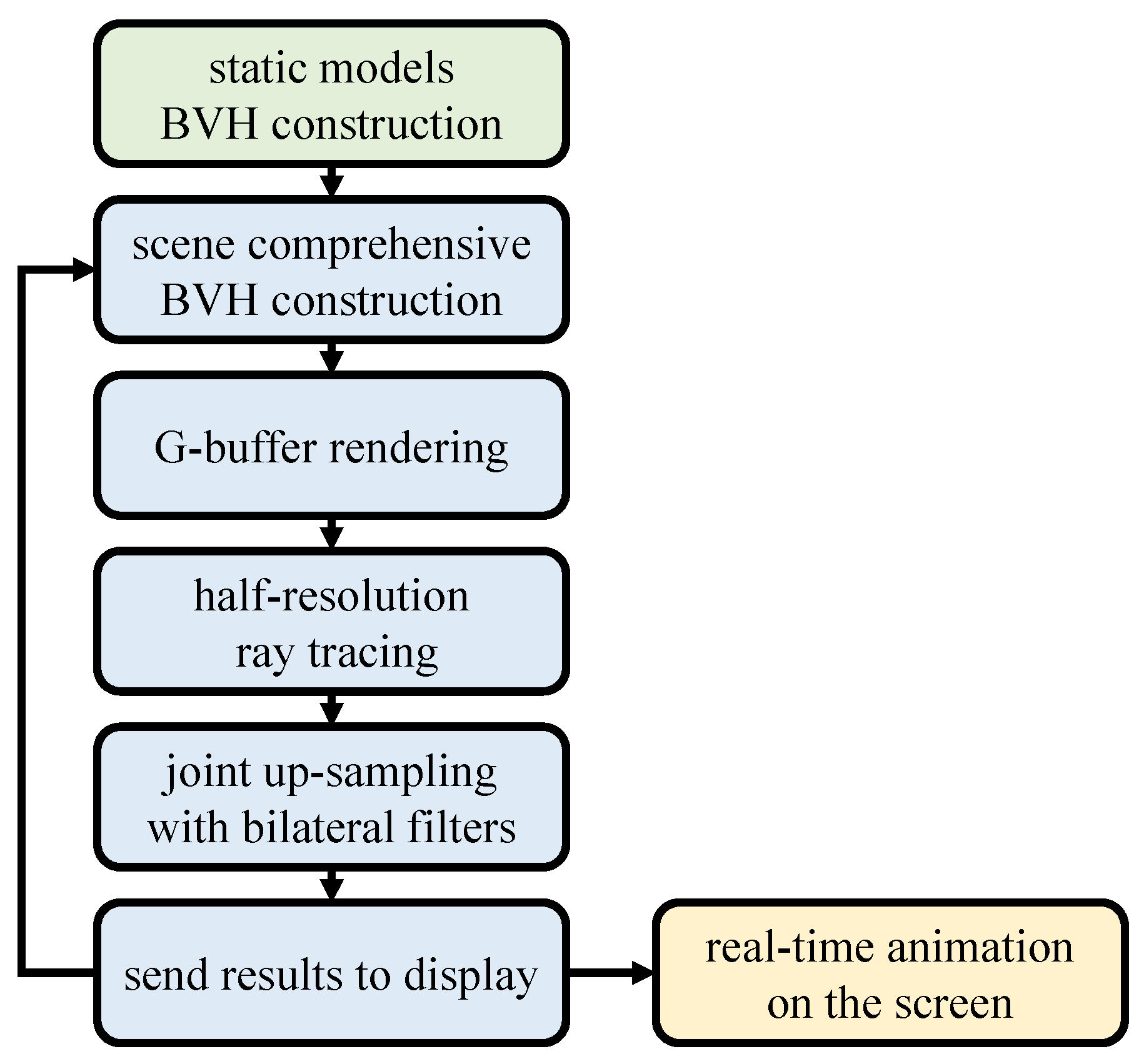
Figure 5 demonstrates the overall architecture of our ray tracing engine. Building the BVH tree takes two steps: per static model construction and scene comprehensive construction. At the beginning, we pre-generate BVH data for static models, referring to the graphical models which do not move or deform its shape in run time. This way we can avoid BVH tree generation overhead on the run. In the next step, we generate a comprehensive BVH tree advantaging from the pre-generated model BVH trees. This procedure is later discussed in Section 3.1 and Section 3.2.
The rest of the part is all performed on the GPU compute shaders and is based on the ray-tracing upsampling method [26]. We compute normal vectors, depth values, and material attributes just as in a deferred rendering pass and followed by the ray-traced illumination approximation. The final rendering composition of the scene is displayed through the frame buffer, and we loop back to the scene comprehensive BVH construction for the next frame until termination. An in-depth explanation of this ray-tracing procedure is in Section 3.3.
3.1. BVH Tree Construction
Bounding Volume Hierarchy is one of the well-known hierarchical approaches to the ray tracing acceleration structures, which handles the operation at a significantly lower cost than without it [23]. It stores the scene data into a binary tree where primitives are recursively wrapped in the bounding volumes, ultimately composing one unified volume on the root of the tree. After its construction, the ray can then traverse down the tree checking intersections with the bounding volume at each node, excluding the primitives which are not in the active ones.
Fast and efficient Boundary Volume Hierarchy tree construction is another interesting aspect of its design. Analysis of its approach is still ongoing despite its aged foundation and is recently aimed at building an inexpensive and dynamic structure for its practical usage [23]. Nonetheless, we implemented a simple bottom-up breadth-first tree generation valuing simpleness over completeness.
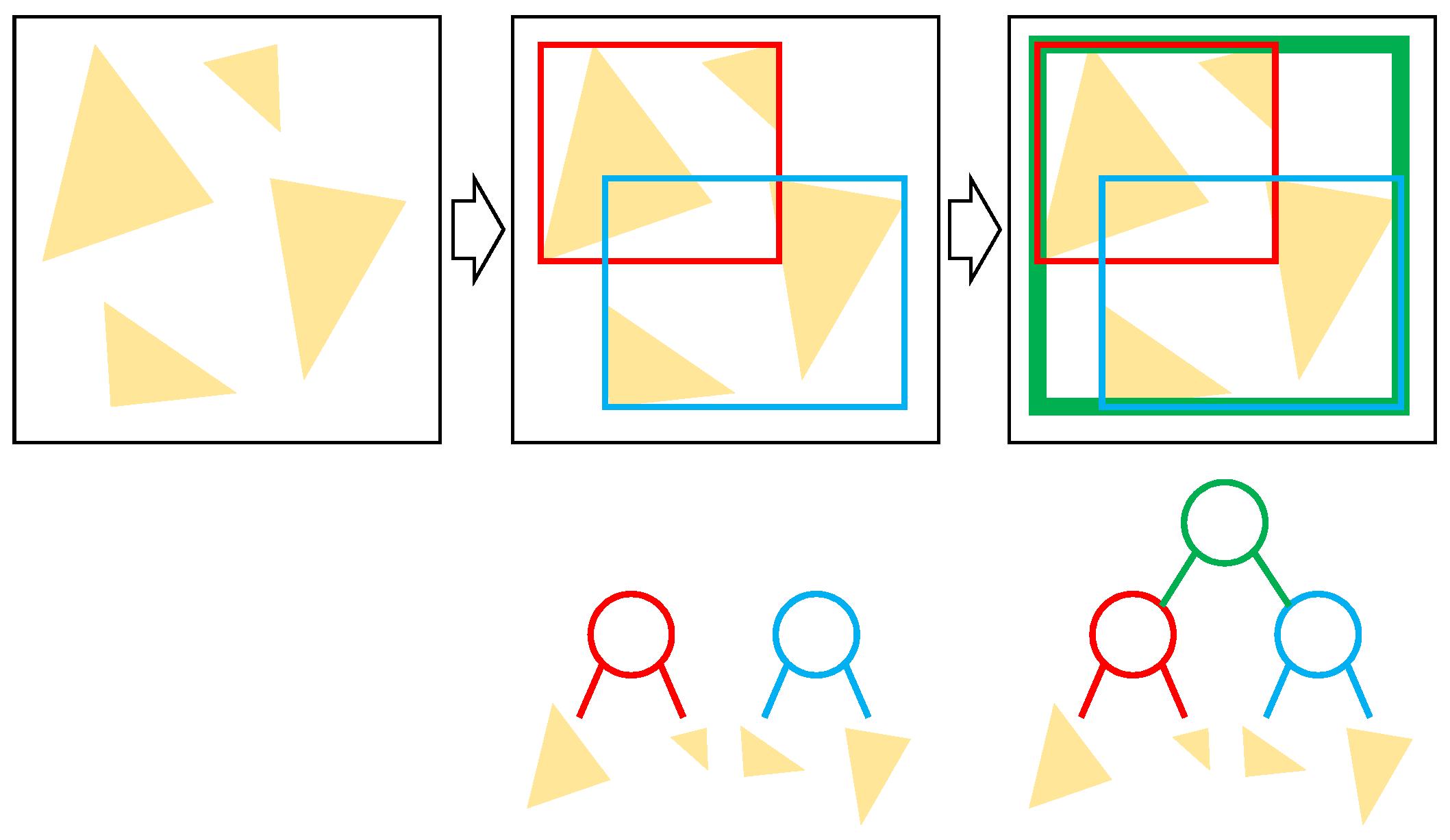
We pair the primitives close to each other’s centroid, leaving a list of single-depth tree nodes, which has the primitives as the child. We then recursively pair the nodes again with the closest centroid, building the tree bottom to top, until it reaches the root node where there are no more nodes to be paired. Figure 6 visualizes this bottom-up breath-first approach.
Although this algorithm provides an efficient enough BVH tree to be traversed, its unstable construction time is a drawback. It has the worst time complexity of , dramatically lowering the performance as the number of primitives n increases.
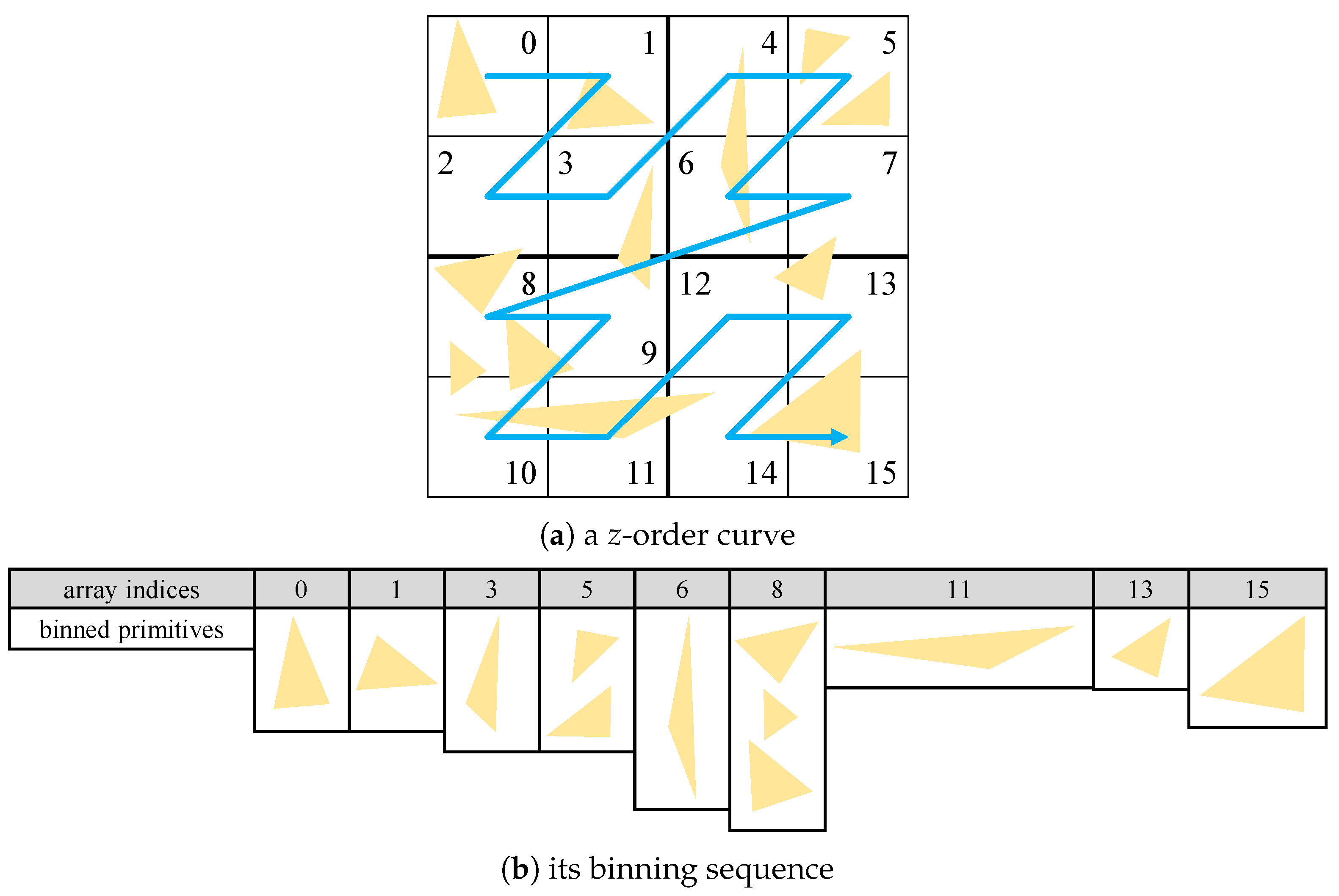
To speed up this process, we exploited Lauterbach’s Morton code method [31]. The space-awareness characteristics of the Morton code, which is also known as the z-order curve, allows us to organize the primitives in the octree hierarchy [28,32]. Primitives are first binned into the z-ordered array indexed by their centroid. Figure 7 explains this z-ordering sequence with a sample 2D quad-tree representation.
Once all the primitives are grouped, we generate BVH trees for each bin and merge them to create one complete tree for the model. This greatly reduces the overhead of closest centroid searching with neglectable precision loss. Our experimental results will be presented in Section 4.
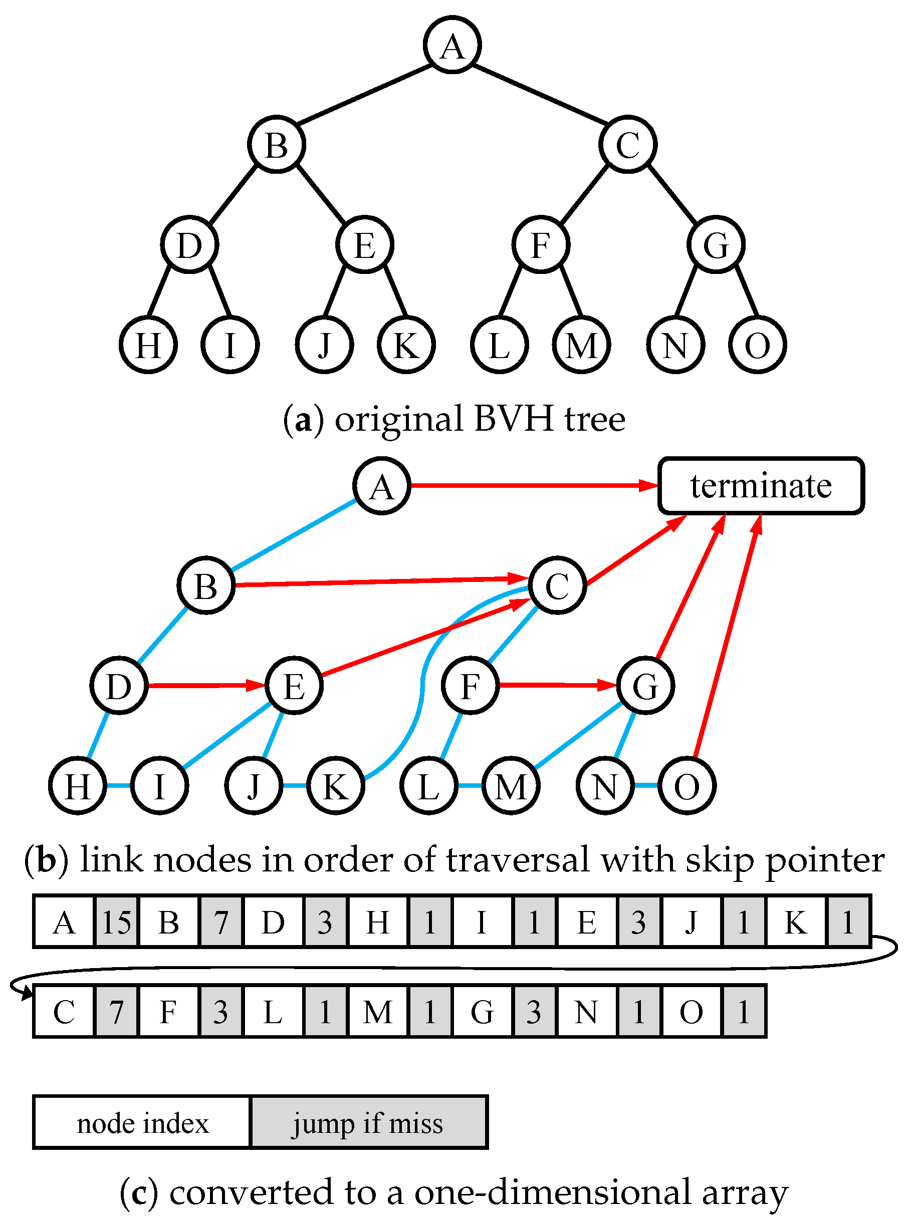
The constructed tree is now transferred to the video memory (VRAM) and hundred millions of rays are evaluated with the compute shader. We found the roped BVH structure to be optimal when sending the tree data to GPU [28,32]; it ensures stackless traversal by storing a skip pointer instead of the parent-sibling tree structure. Figure 8 demonstrates the creation of an example roped BVH, in a step by step manner [33,34]. Blue lines represent the tree traversal in the left-to-right order, while red arrows represent skip pointers where iteration will skip to when the current volume is not hit. After linking the nodes by the traversal order, we convert the tree into an array and send it to the GPU as a texture. The tree will be traversed with the code in Pseudocode 1.
Pseudocode 1. Pseudo code for the Roped BVH tree traversal.
| i = 0 |
| whilei < bvh.size(): |
| if bvh[i] is a primitive: |
| perform and record the ray-object intersection check |
| else if the ray does not hit the bounding volume of bvh[i]: |
| i += bvh[i].skip_index |
| else: |
| i++ |
3.2. Dynamic Object Handling
Generating a BVH tree for the entire scene is still a hard work if there are millions of primitives to render. We might have scenes with many duplicate models such as trees in the forest or houses in the town. To reduce such overhead, we generate two types of BVH trees: per-static model construction and scene comprehensive construction.
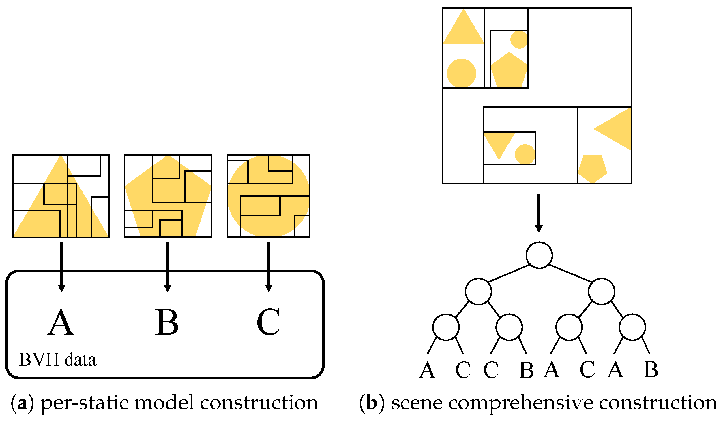
The former one, performed before the rendering loop, creates an unmodifiable object space BVH tree per model. Its leaf nodes contain the pointer to the graphics primitives based on non-animated model files, as shown in Figure 9a. These per-static models act as the object pool, for duplicated static objects.
The latter performs the world space BVH tree building, addressing all the objects inside the scene with the model pointers. Unlike the static model ones, this tree has the pointer to the corresponding pre-processed model and the corresponding transformation matrix to save both space and time for the rendering.
The per-static individual model BVH trees are pre-processed and stored in a 2D image array, and the scene comprehensive tree references them at the leaf nodes. To handle the moving and/or deformable objects, the scene comprehensive tree is reconstructed every time at the beginning of the rendering loop. Since we can enjoy the time-coherency of the scenes, we can partially update the scene comprehensive tree, with respect to the moving and/or deformable objects.
3.3. Ray Reflection Calculation
The light transport calculation is another important point of the ray-tracing method, as the ray reflection calculation step [27,28]. Many illumination calculation methods are available, starting from physically correct BRDF (bidirectional reflectance distribution function) and BSDF (bidirectional scattering distribution function) formula to diverse artistic approaches including cell-shading and more.
We opted for one of the most efficient illumination methods:
where is the illumination of the current ray R and its hit surface S. Upon hit, the surface’s light emittance and attenuation is calculated into the traced light color. After the intersection, a new ray reflected from the surface S and its new hit surface is recursively attained to trace the next ray illumination .
To overcome the high computation burden of the ray-tracing, we adopted Boughida’s upsampling method [31]. The main idea is to improve performance by reducing the number of pixels to compute.
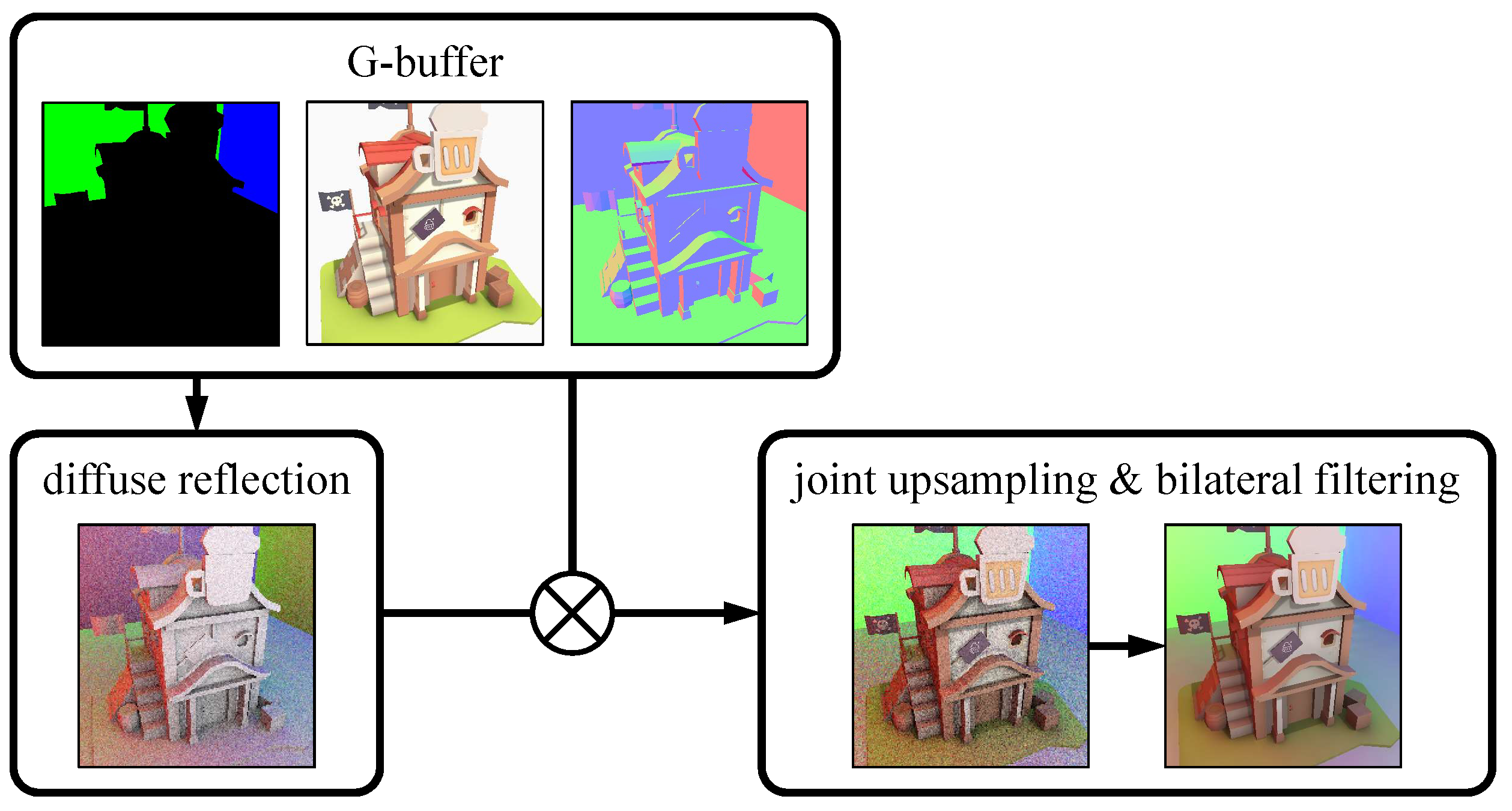
Figure 10 depicts the detail of our rendering process. We first generate the full resolution G-buffer. The G-buffer is a collection of all lighting-relevant textures produced to compose the final lighting pass, which is an essential step for all deferred rendering pipelines [35,36]. The G-buffer includes normal vectors, depth values, and material information of the rendered image. Material data carries its surface image, roughness, and emittance. These textures can be generated through a conventional rasterization pipeline since it does not involve indirect lighting. In this work, we decided to use the compute shader-based ray casting for efficiency. We then compute the ray-traced indirect illumination in a half-resolution and upsample it back to the full resolution based on these pre-generated G-buffer images.
We used edge-preserving joint bilateral upsampling to avoid the flaws of fuzzy and noisy upsampling [37,38,39]. We upsample the low-resolution image with the help of full-resolution normal vector and depth value information, preserving the notable edges.
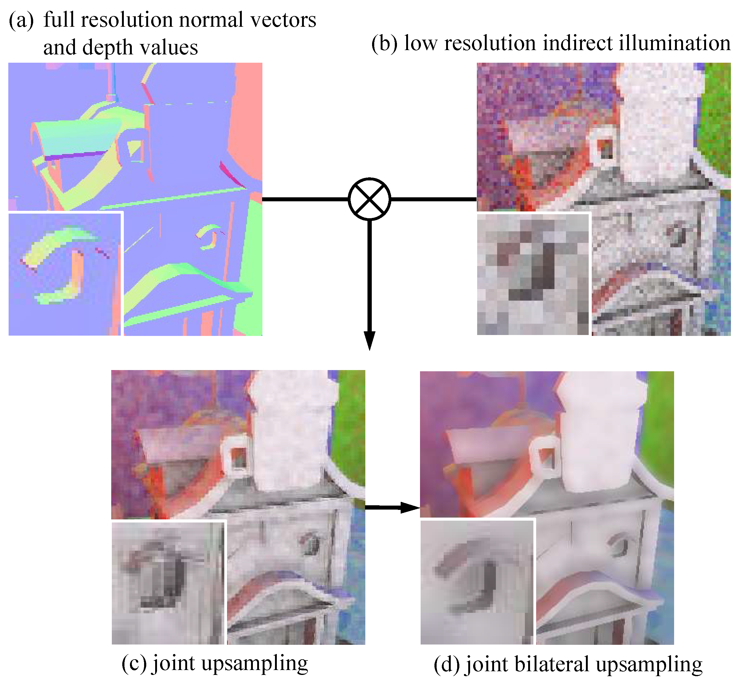
Figure 11 depicts the difference between these methods. Joint bilateral upsampling is one derivation of the bilateral filtering method, utilizing both spatial and range filter kernel [40,41]. The final color composition of the pixel at the pixel position p in the spatial kernel can be denoted as below:
where is the normalization factor and f, g is the spatial and range filter kernel, respectively. Unlike the conventional bilateral filter, the joint bilateral upsampling uses the guidance image G to evaluate the range factor, which is normal vector and depth value images in our case.
The spatial kernel f is a truncated Gaussian function and is pre-computed before the run-time usage:
where s is the kernel size. The range kernel g is the edge-preserving factor evaluated by the G-buffer normal vector n and depth value z:
4. Implementation Results
Our ray-tracing engine runs on Windows 10 and is based on the C++ programming language with Visual Studio 2019 development environment. The OpenGL graphics library [44,45] has opted for more elegant codes. The rendering environment is Nvidia GeForce GTX 1070 graphics card and Intel Core i7-6700K 4.00 GHz CPU.
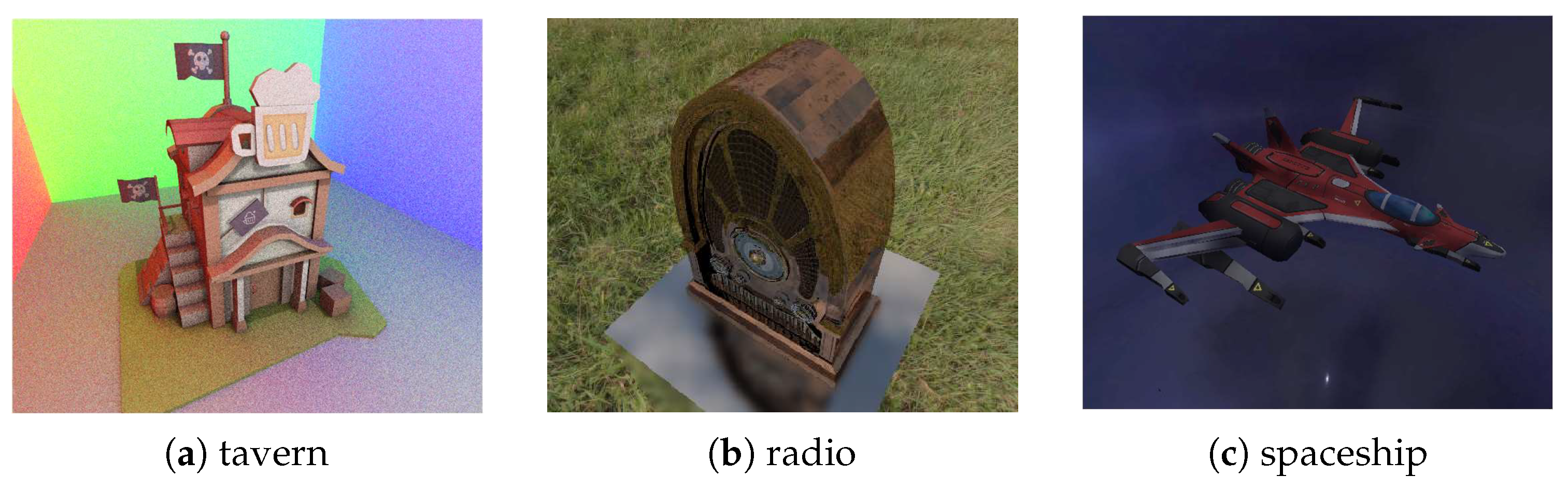
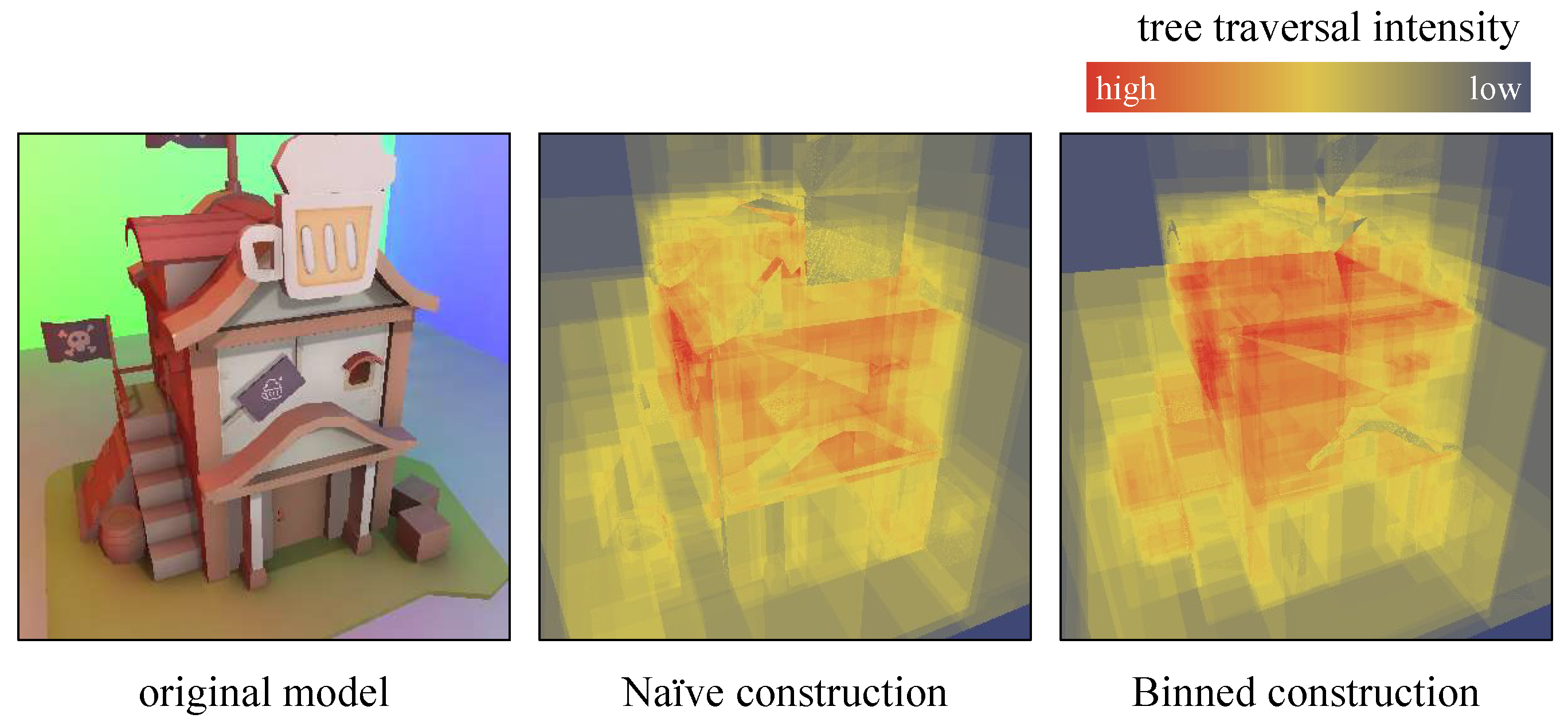
To analyze our implementation, we used three different animation scenes for the test cases: tavern, radio, and spaceship, as shown in Figure 12. As presented in Figure 5 and Section 3.1, our implementation starts from constructing BVH trees, for overall speed-ups. The heat map in Figure 13 proves that the binned BVH tree structure is consistent to the original tree, which was constructed without accelerated binning techniques.
Table 1 is the performance result of the tree construction with and without primitive binning. Results are evaluated by averaging 100 tests per model. Table 1 shows that the binned construction is 6.631 to 16.391 times accelerated. Note that this result is only for the BVH tree construction. We should include the reflection calculation steps.
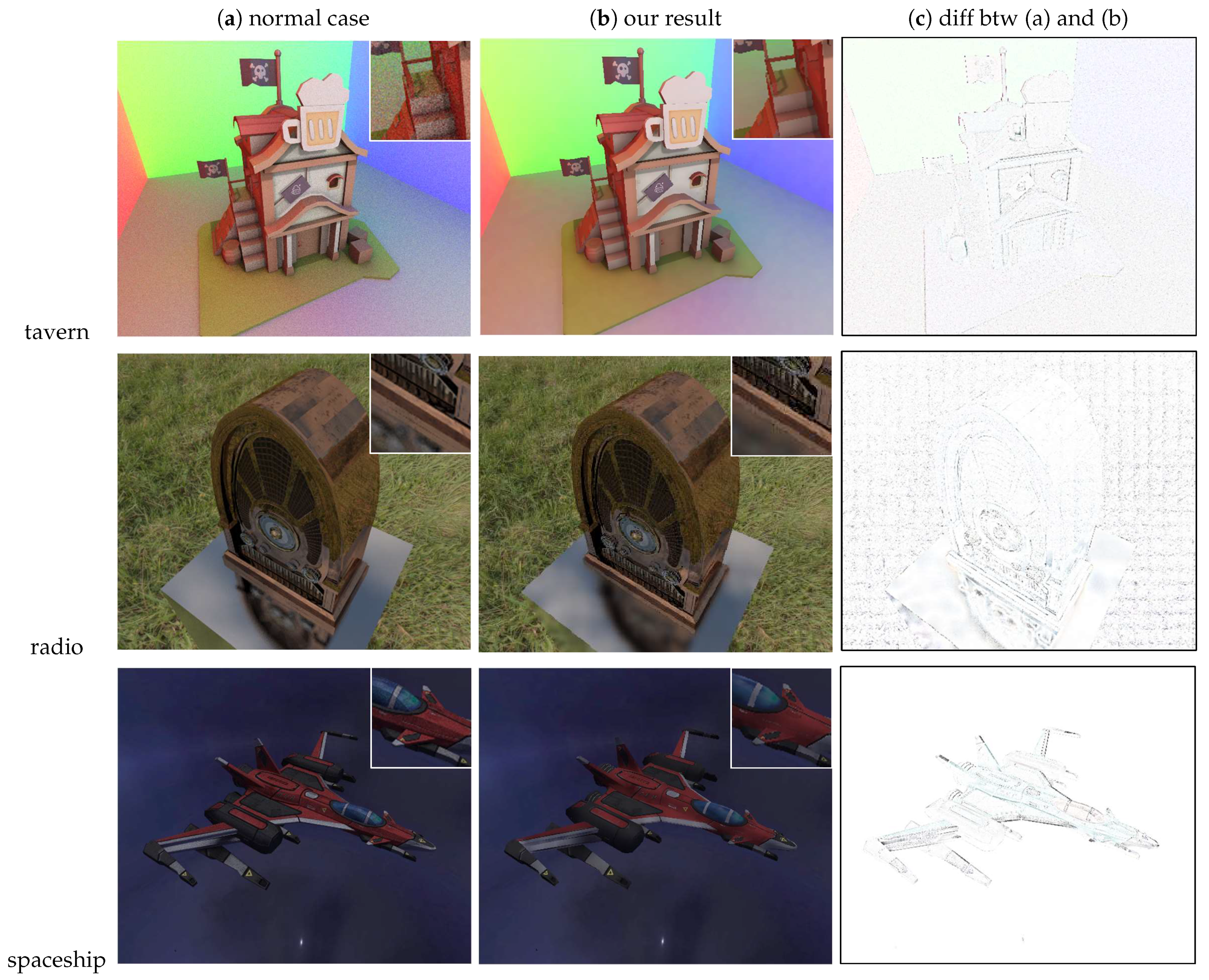
We were able to achieve modest interactive ray traced illumination with the OpenGL compute shader, as shown in Figure 14. The roped BVH acceleration structure and the upsampling technique enabled us to boost rendering performance. All scenes were rendered with 2 ray bounce limit and 100 sampling in its resolution. Note that the ray bounce count and the ray sampling count are the important control factors for the speed of the overall ray-tracing process. With our current hardware configuration, 2 ray bounces and 100 samplings per pixel are the limits for real-time processing.
Figure 14 and Table 2 shows the rendering result and performance of our experimental scenes. Figure 14a shows the normal ray-traced images, without roped BVH acceleration and upsampling techniques. Figure 14b represents our ray-traced results with all acceleration techniques are applied. Figure 14c represents the pixel-by-pixel differences between Figure 14a,b.
The rendering performances are shown in Table 2. The final acceleration ratio shows that our final results are accelerated at least 2.478 to 13.618 times (maximum). The pixel-by-pixel error measures are shown in Table 3. We denoted the errors as percent values with respect to the pixel value ranges. Since we use 256-levels for each color channels, the 50% error means 128 level differences in its absolute pixel values.
As shown in Table 2, the error values show the mean values () from 0.215% to 0.854%, and standard deviations () from 0.680% to 0.990%, as their statistical values. Assuming the normal distributions, we can expect that more than 95% of the pixel-by-pixel errors are less than the value of , or 1.977%–2.767%. Finally, we can expect that almost pixel-by-pixel errors are bound less than 3% of the actual pixel values.
In the case of minimum and maximum error values, we have some outliers, unfortunately. Table 2 shows that at most 77% error was found, as one of the worst cases. Fortunately, they are very restricted cases to the sharp edge areas, due to the limitations of the joint bilateral upsampling. At the edge boundaries, the joint bilateral upsampling cannot avoid to fail the accurate ray-object intersections and also ray-reflection calculations. These artifacts are drawbacks of our acceleration scheme, and will be investigated in the future.
5. Conclusions and Future Work
In this paper, we present the overall details of our real-time ray-traced rendering engine. To achieve the real-time ray-traced rendering, we applied a set of acceleration techniques, including the bounding volume hierarchy, its roped representation, joint up-sampling, and bilateral filtering. Additionally, for more speed-ups, we implemented these features on the GPU compute shaders. Finally, we get 2.5–13.6 times accelerations, and real-time rendering, for all of our test cases.
Actually, we now achieved a ray-traced rendering framework, and we can apply much more experimental works. For example, since we used the shader programs to achieve the real-time ray-tracing, we can simultaneously apply some shader-based special effects, including cartoon rendering and high-dynamic range rendering. Various experimental combinations of ray-tracing frameworks and shader-based rendering techniques can be our future works.
For the implementation point of view, we can achieve more speed-ups through concentrating on the faster BVH construction, and/or tree traversal. Reducing the pixel-by-pixel artifacts can also be investigated in near future.
Author Contributions
Software, writing—original draft presentation, visualization, S.P.; Conceptualization, methodology, investigation, writing—review and editing, supervision, funding acquisition, N.B. All authors have read and agreed to the published version of the manuscript.
Funding
This work was supported by Basic Science Research Program through the National Research Foundation of Korea (NRF) funded by the Ministry of Education (Grand No. NRF-2019R1I1A3A01061310). This study was also supported by the BK21 FOUR project (AI-driven Convergence Software Education Research Program) funded by the Ministry of Education, School of Computer Science and Engineering, Kyungpook National University, Korea (4199990214394).
Institutional Review Board Statement
Not applicable.
Informed Consent Statement
Not applicable.
Data Availability Statement
The data presented in this study are available on request from the corresponding author.
Conflicts of Interest
The authors declare no conflict of interest.
References
- Baek, N.; Kim, K. Design and implementation of OpenGL SC 2.0 rendering pipeline. Clust. Comput. 2019, 22, 931–936. [Google Scholar] [CrossRef]
- Baek, N. An emulation scheme for OpenGL SC 2.0 over OpenGL. J. Supercomput. 2020, 76, 7951–7960. [Google Scholar] [CrossRef]
- McGuire, M.; Shirley, P.; Wyman, C. Introduction to Real-Time Ray Tracing. In Proceedings of the ACM SIGGRAPH 2019 Courses, Los Angeles, CA, USA, 28 July 2019. [Google Scholar] [CrossRef]
- Glassner, A.S. (Ed.) An Introduction to Ray Tracing; Academic Press Ltd.: Cambridge, MA, USA, 1989. [Google Scholar]
- Whitted, T. An Improved Illumination Model for Shaded Display. In Proceedings of the ACM SIGGRAPH 2005 Courses, Los Angeles, CA, USA, 31 July–4 August 2005. [Google Scholar] [CrossRef] [Green Version]
- Buck, J. The Ray Tracer Challenge: A Test-Driven Guide to Your First 3D Renderer; Pragmatic Bookshelf: Raleigh, NC, USA, 2019. [Google Scholar]
- Kim, D.; Kim, L.S. Area-efficient pixel rasterization and texture coordinate interpolation. Comput. Graph. 2008, 32, 669–681. [Google Scholar] [CrossRef]
- Haines, E.; Akenine-Möller, T. (Eds.) Ray Tracing Gems; Apress: New York, NY, USA, 2019; Available online: http://raytracinggems.com (accessed on 30 March 2021).
- Ward, G.; Reinhard, E.; Debevec, P. High Dynamic Range Imaging and Image-Based Lighting. In Proceedings of the ACM SIGGRAPH 2008 Classes, Los Angeles, CA, USA, 11–15 August 2008. [Google Scholar] [CrossRef]
- Ward, G.J.; Clear, R.D. A Ray Tracing Solution for Diffuse Interreflection. In Proceedings of the ACM SIGGRAPH 2008 Classes, Los Angeles, CA, USA, 11–15 August 2008. [Google Scholar] [CrossRef]
- McGuire, M.; Mara, M.; Nowrouzezahrai, D.; Luebke, D. Real-Time Global Illumination Using Precomputed Light Field Probes. In Proceedings of the 21st ACM SIGGRAPH Symposium on Interactive 3D Graphics and Games, San Francisco, CA, USA, 4–5 March 2017. [Google Scholar] [CrossRef]
- Ritschel, T.; Grosch, T.; Seidel, H.P. Approximating Dynamic Global Illumination in Image Space. In Proceedings of the 2009 Symposium on Interactive 3D Graphics and Games, Costa Mesa, CA, USA, 7–14 February 2009; pp. 75–82. [Google Scholar] [CrossRef]
- Thiedemann, S.; Henrich, N.; Grosch, T.; Müller, S. Voxel-Based Global Illumination. In Proceedings of the Symposium on Interactive 3D Graphics and Games, San Francisco, CA, USA, 18–20 February 2011; pp. 103–110. [Google Scholar] [CrossRef] [Green Version]
- Luksch, C.; Wimmer, M.; Schwärzler, M. Incrementally Baked Global Illumination. In Proceedings of the ACM SIGGRAPH Symposium on Interactive 3D Graphics and Games, San Francisco, CA, USA, 25–27 February 2019. [Google Scholar] [CrossRef] [Green Version]
- Kaplanyan, A.S.; Dachsbacher, C. Adaptive Progressive Photon Mapping. ACM Trans. Graph. 2013, 32. [Google Scholar] [CrossRef]
- Kang, C.; Wang, L.; Meng, X.; Xu, Y. Progressive Photon Mapping with Sample Elimination. In Proceedings of the 20th ACM SIGGRAPH Symposium on Interactive 3D Graphics and Games, Redmond, WA, USA, 26–28 February 2016; p. 201. [Google Scholar] [CrossRef]
- Baek, N.; Yoo, K. Emulating OpenGL ES 2.0 over the desktop OpenGL. Clust. Comput. 2015, 18, 165–175. [Google Scholar] [CrossRef]
- Baek, N.; Kim, K.J. An artifact detection scheme with CUDA-based image operations. Clust. Comput. 2017, 20, 749–755. [Google Scholar] [CrossRef]
- Meister, D.; Boksansky, J.; Guthe, M.; Bittner, J. On Ray Reordering Techniques for Faster GPU Ray Tracing. In Proceedings of the Symposium on Interactive 3D Graphics and Games, San Francisco, CA, USA, 15–17 September 2020. [Google Scholar] [CrossRef]
- Gordon, V.S.; Clevenger, J. Computer Graphics Programming in OpenGL with C++, 2nd ed.; Mercury Learning and Information: Duxbury, MA, USA, 2020. [Google Scholar]
- Zhu, M.; House, D.; Carlson, M. Ray Casting Sparse Level Sets. In Proceedings of the Digital Production Symposium, Los Angeles, CA, USA, 4 August 2012; pp. 67–72. [Google Scholar] [CrossRef]
- Gavrilov, N.; Turlapov, V. Advanced GPU-Based Ray Casting for Bricked Datasets. In Proceedings of the ACM SIGGRAPH 2012 Posters, Los Angeles, CA, USA, 7–9 August 2012. [Google Scholar] [CrossRef]
- Sousa, N.; Sena, D.; Papadopoulos, N.; Pereira, J. Acceleration Data Structures for Ray Tracing on Mobile Devices. In Proceedings of the 14th International Joint Conference on Computer Vision, Imaging and Computer Graphics Theory and Applications—Volume 1, Prague, Czech Republic, 25–27 February 2019; pp. 332–339. [Google Scholar] [CrossRef]
- Popov, S.; Günther, J.; Seidel, H.P.; Slusallek, P. Stackless KD-Tree Traversal for High Performance GPU Ray Tracing. Comput. Graph. Forum 2007, 26, 415–424. [Google Scholar] [CrossRef]
- Bulavintsev, V.; Zhdanov, D. Constructing K-d Tree on GPU through Treelet Restructuring. In Proceedings of the 30th International Conference on Computer Graphics and Machine Vision (GraphiCon 2020), Part 2, St. Petersburg, Russia, 22–25 September 2020. [Google Scholar] [CrossRef]
- Smits, B. Efficiency Issues for Ray Tracing. J. Graph. Tools 1998, 3, 1–14. [Google Scholar] [CrossRef]
- Domingues, L.R.; Pedrini, H. Bounding Volume Hierarchy Optimization through Agglomerative Treelet Restructuring. In Proceedings of the 7th Conference on High-Performance Graphics, Los Angeles, CA, USA, 7–9 August 2015; pp. 13–20. [Google Scholar] [CrossRef]
- Sieranoja, S.; Fränti, P. Constructing a High-Dimensional kNN-Graph Using a Z-Order Curve. ACM J. Exp. Algorithm. 2018, 23. [Google Scholar] [CrossRef]
- Burgess, J. RTX on the NVIDIA Turing GPU. IEEE Micro 2020, 40, 36–44. [Google Scholar] [CrossRef]
- Sanders, A. An Introduction to Unreal Engine 4; CRC Press: Boca Raton, FL, USA, 2016. [Google Scholar]
- Lauterbach, C.; Garland, M.; Sengupta, S.; Luebke, D.; Manocha, D. Fast BVH Construction on GPUs. Comput. Graph. Forum 2009. [Google Scholar] [CrossRef]
- Morton, G. A Computer Oriented Geodetic Data Base and a New Technique in File Sequencing; International Business Machines Company: Armonk, NY, USA, 1966. [Google Scholar]
- Vinkler, M.; Havran, V.; Bittner, J. Performance Comparison of Bounding Volume Hierarchies and Kd-Trees for GPU Ray Tracing. Comput. Graph. Forum 2015, 35, 68–79. [Google Scholar] [CrossRef]
- Torres, R.; Martín, P.J.; Gavilanes, A. Ray Casting Using a Roped BVH with CUDA. In Proceedings of the 25th Spring Conference on Computer Graphics, Budmerice, Slovakia, 23–25 April 2009; pp. 95–102. [Google Scholar] [CrossRef]
- Crassin, C.; McGuire, M.; Fatahalian, K.; Lefohn, A. Aggregate G-Buffer Anti-Aliasing. In Proceedings of the 19th Symposium on Interactive 3D Graphics and Games, Costa Mesa, CA, USA, 9–11 March 2015; pp. 109–119. [Google Scholar] [CrossRef]
- Klint, J. Deferred Rendering in Leadwerks Engine; Leadwerks Corporation: Las Vegas, NV, USA, 2008. [Google Scholar]
- Chen, J.; Adams, A.; Wadhwa, N.; Hasinoff, S.W. Bilateral Guided Upsampling. ACM Trans. Graph. 2016, 35. [Google Scholar] [CrossRef] [Green Version]
- Kopf, J.; Cohen, M.F.; Lischinski, D.; Uyttendaele, M. Joint Bilateral Upsampling. ACM Trans. Graph. 2007, 26, 96. [Google Scholar] [CrossRef]
- Boughida, M.; Groueix, T.; Boubekeur, T. Interactive Monte-Carlo Ray-Tracing Upsampling. In EG 2016—Posters; Magalhaes, L.G., Mantiuk, R., Eds.; The Eurographics Association: Norkoping, Sweden, 2016. [Google Scholar] [CrossRef]
- Paris, S.; Kornprobst, P.; Tumblin, J.; Durand, F. A Gentle Introduction to Bilateral Filtering and Its Applications. In Proceedings of the ACM SIGGRAPH 2008 Classes, Los Angeles, CA, USA, 11–15 August 2008. [Google Scholar] [CrossRef]
- Park, M.K.; Cho, J.H.; Jang, I.Y.; Lee, S.J.; Lee, K.H. An Iterative Joint Bilateral Filtering for Depth Refinement of a 3D Model. In Proceedings of the SIGGRAPH Asia 2011 Posters, Hong Kong, China, 12–15 December 2011. [Google Scholar] [CrossRef]
- Luna, F. Introduction to 3D Game Programming with DirectX; Mercury Learning and Information: Duxbury, MA, USA, 2012. [Google Scholar]
- Bilodeau, B. Efficient Compute Shader Programming; AMD: San Francisco, CA, USA, 2011. [Google Scholar]
- Segal, M.; Akeley, K. The OpenGL Graphics System: A Specification, Version 4.6; Khronos Group: Beaverton, WA, USA, 2019. [Google Scholar]
- Kessenich, J. The OpenGL Shading Language, Version 4.60; Khronos Group: Beaverton, WA, USA, 2019. [Google Scholar]
Figure 1.
Example pictures of the traditional rasterization and the ray-traced rendering.

Figure 2.
Differences between the specular and diffuse reflections: specuclar reflections occur on mirror-like surfaces, while diffuse reflections shows light scattering effects.
Figure 2.
Differences between the specular and diffuse reflections: specuclar reflections occur on mirror-like surfaces, while diffuse reflections shows light scattering effects.

Figure 3.
Results of different ray sampling counts: High samples per pixel (spp) values give high quality images, with large amount of computing time (in msec).
Figure 3.
Results of different ray sampling counts: High samples per pixel (spp) values give high quality images, with large amount of computing time (in msec).

Figure 4.
Visualization of two major acceleration methods.

Figure 5.
Overview of our ray tracing engine.

Figure 6.
A simple 2D example of the bottom-up breath-first tree construction: closer objects are paired until the whole space is processed into the tree.
Figure 6.
A simple 2D example of the bottom-up breath-first tree construction: closer objects are paired until the whole space is processed into the tree.

Figure 7.
A z-order sequence marked on the 2D quad-tree representation, and its corresponding Morton-ordered binning sequence.
Figure 7.
A z-order sequence marked on the 2D quad-tree representation, and its corresponding Morton-ordered binning sequence.

Figure 8.
Constructing the roped BVH tree: blue lines denote the left-to-right traversal, while red arrows show the skip pointers.
Figure 8.
Constructing the roped BVH tree: blue lines denote the left-to-right traversal, while red arrows show the skip pointers.

Figure 9.
Two separate BVH tree constructions: the scene comprehensive construction uses the per-static models as the pre-processed and duplicated models.
Figure 9.
Two separate BVH tree constructions: the scene comprehensive construction uses the per-static models as the pre-processed and duplicated models.

Figure 10.
Our rendering pipeline in order.

Figure 11.
Joint upsampling results.

Figure 12.
Three different scenes for test cases.

Figure 13.
BVH tree structures, compared with respect to the heat map.

Figure 14.
Our rendering results for three different scenes with 2 ray bounce and 100 sample limits.
Figure 14.
Our rendering results for three different scenes with 2 ray bounce and 100 sample limits.


Table 1.
The BVH tree construction performance for three different models (unit: μsec).
| (a) Naive | (b) Binned | Acceleration | |
|---|---|---|---|
| Construction | Construction | Ratio | |
| (Prev Method) | (Our Method) | (a)/(b) | |
| tavern | 137,847 | 20,787 | 6.631 |
| radio | 281,897 | 20,172 | 13.974 |
| spaceship | 262,211 | 15,996 | 16.391 |
Table 2.
Performance of our rendering results (unit: μsec).
| (a) Normal Case | (b) Our Result | (c) Accel Ratio (a)/(b) | |
|---|---|---|---|
| tavern | 1,352,951 | 545,824 | 2.478 |
| radio | 313,094 | 22,991 | 13.618 |
| spaceship | 322,434 | 28,759 | 11.211 |
Table 3.
Error analysis for differences.
| Mean (μ) | Std Dev () | 2 Range | Min | Max | |
|---|---|---|---|---|---|
| tavern | 0.854% | 0.680% | 2.214% | 0.000% | 77.344% |
| radio | 0.788% | 0.990% | 2.767% | 0.000% | 66.797% |
| spaceship | 0.215% | 0.881% | 1.977% | 0.000% | 70.703% |
Publisher’s Note: MDPI stays neutral with regard to jurisdictional claims in published maps and institutional affiliations. |
© 2021 by the authors. Licensee MDPI, Basel, Switzerland. This article is an open access article distributed under the terms and conditions of the Creative Commons Attribution (CC BY) license (https://creativecommons.org/licenses/by/4.0/).
Share and Cite
MDPI and ACS Style
Park, S.; Baek, N. A Shader-Based Ray Tracing Engine. Appl. Sci. 2021, 11, 3264. https://doi.org/10.3390/app11073264
AMA Style
Park S, Baek N. A Shader-Based Ray Tracing Engine. Applied Sciences. 2021; 11(7):3264. https://doi.org/10.3390/app11073264
Chicago/Turabian StylePark, Sukjun, and Nakhoon Baek. 2021. "A Shader-Based Ray Tracing Engine" Applied Sciences 11, no. 7: 3264. https://doi.org/10.3390/app11073264
Note that from the first issue of 2016, this journal uses article numbers instead of page numbers. See further details here.