
COVID-19 Diagnosis in Chest X-rays Using Deep Learning and Majority Voting


Abstract
:1. Introduction
1.1. COVID-19 Diagnosis in Chest X-rays Images
1.2. Related Works
2. Materials & Methods
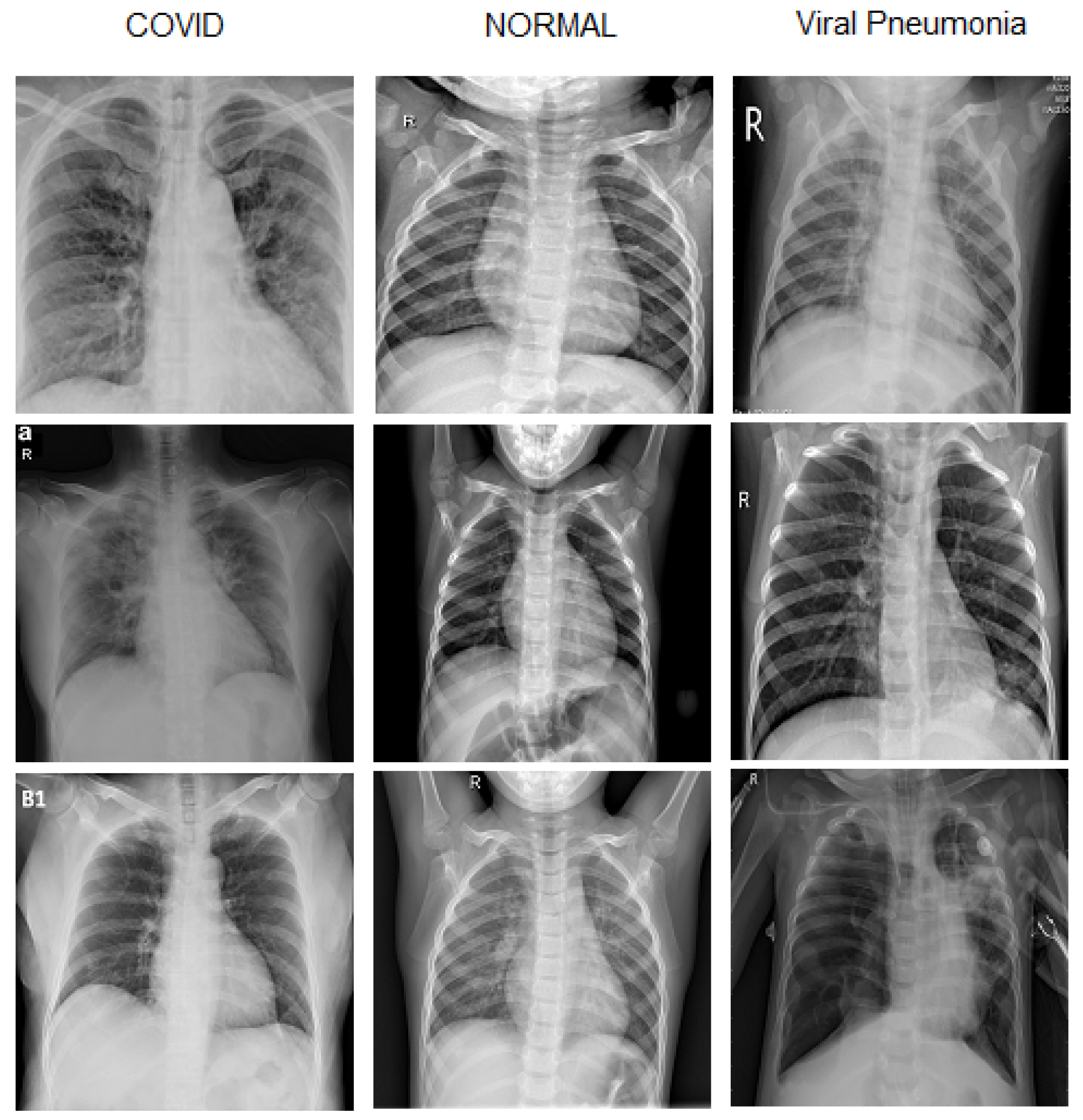
2.1. Dataset Preparation
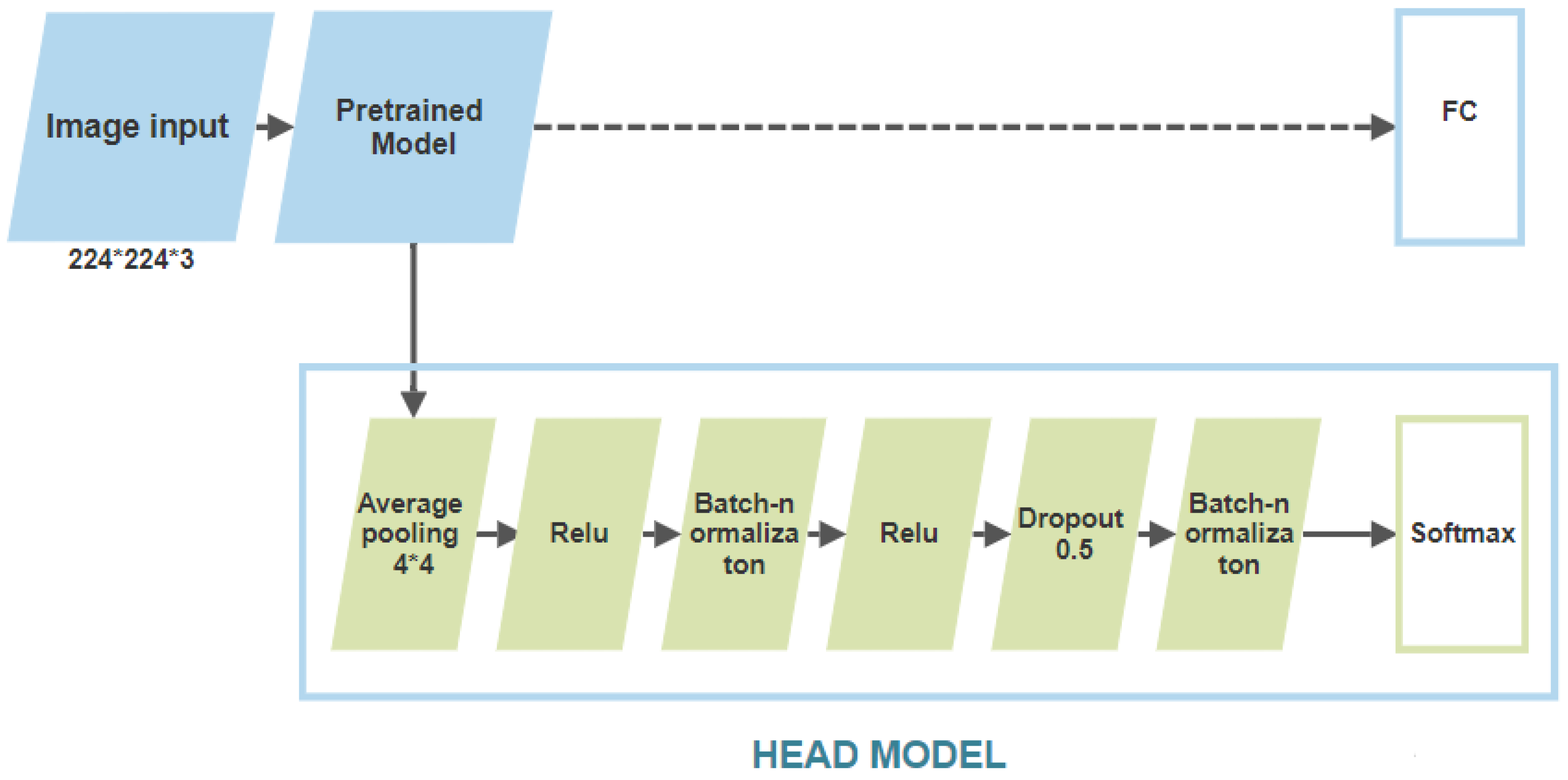
2.2. Training of the Selected Algorithms
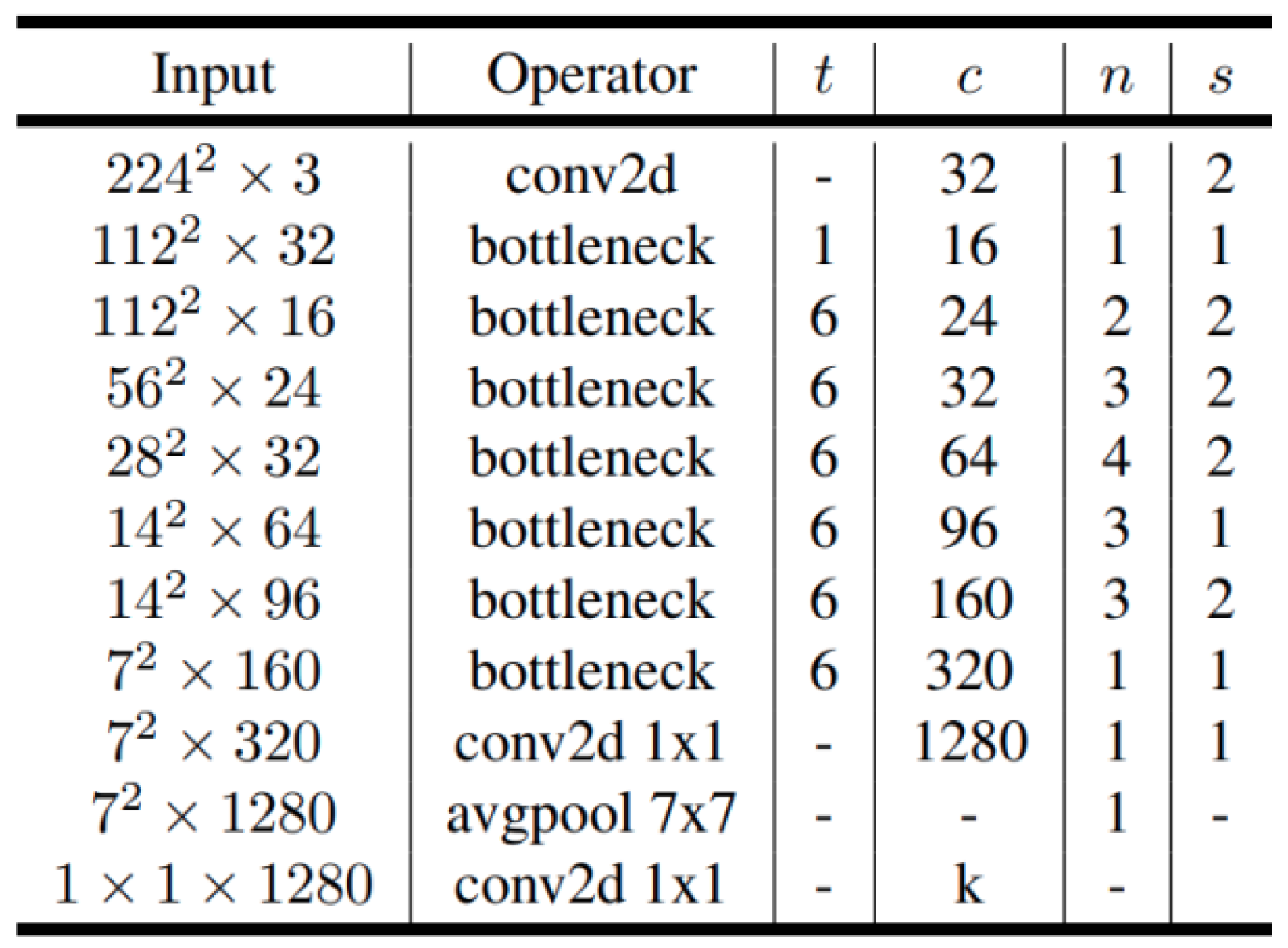
2.2.1. MobileNet
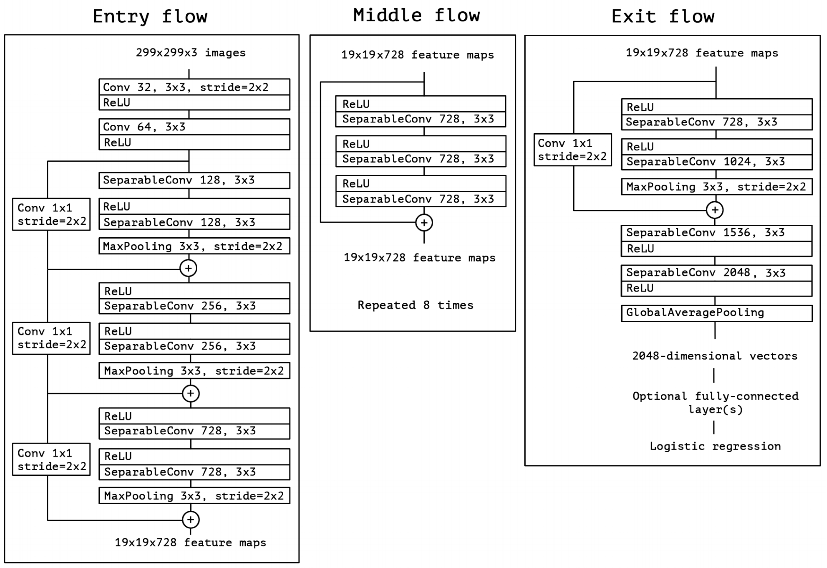
2.2.2. Xception
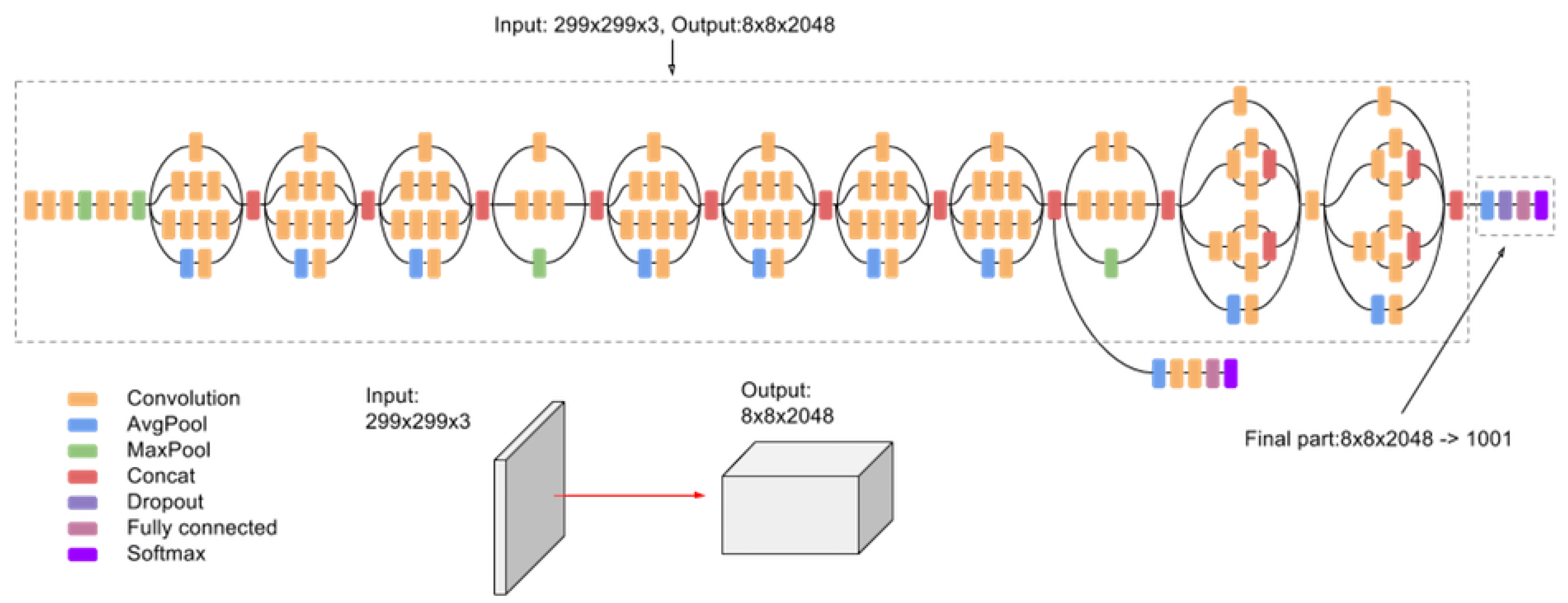
2.2.3. Inception
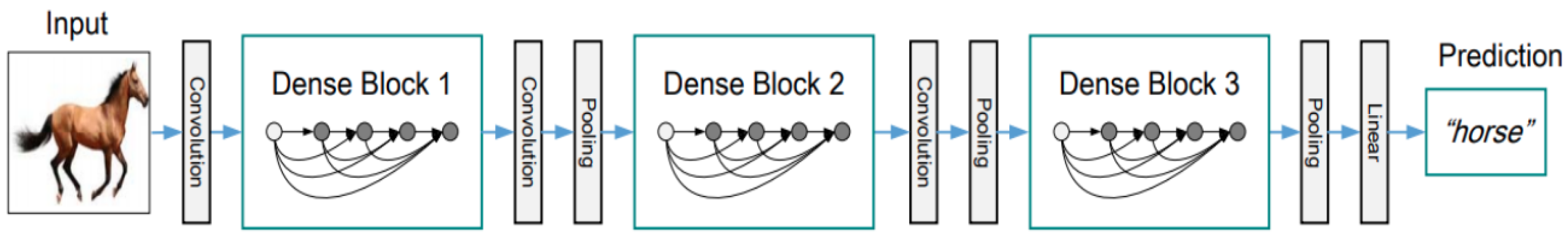
2.2.4. DenseNet
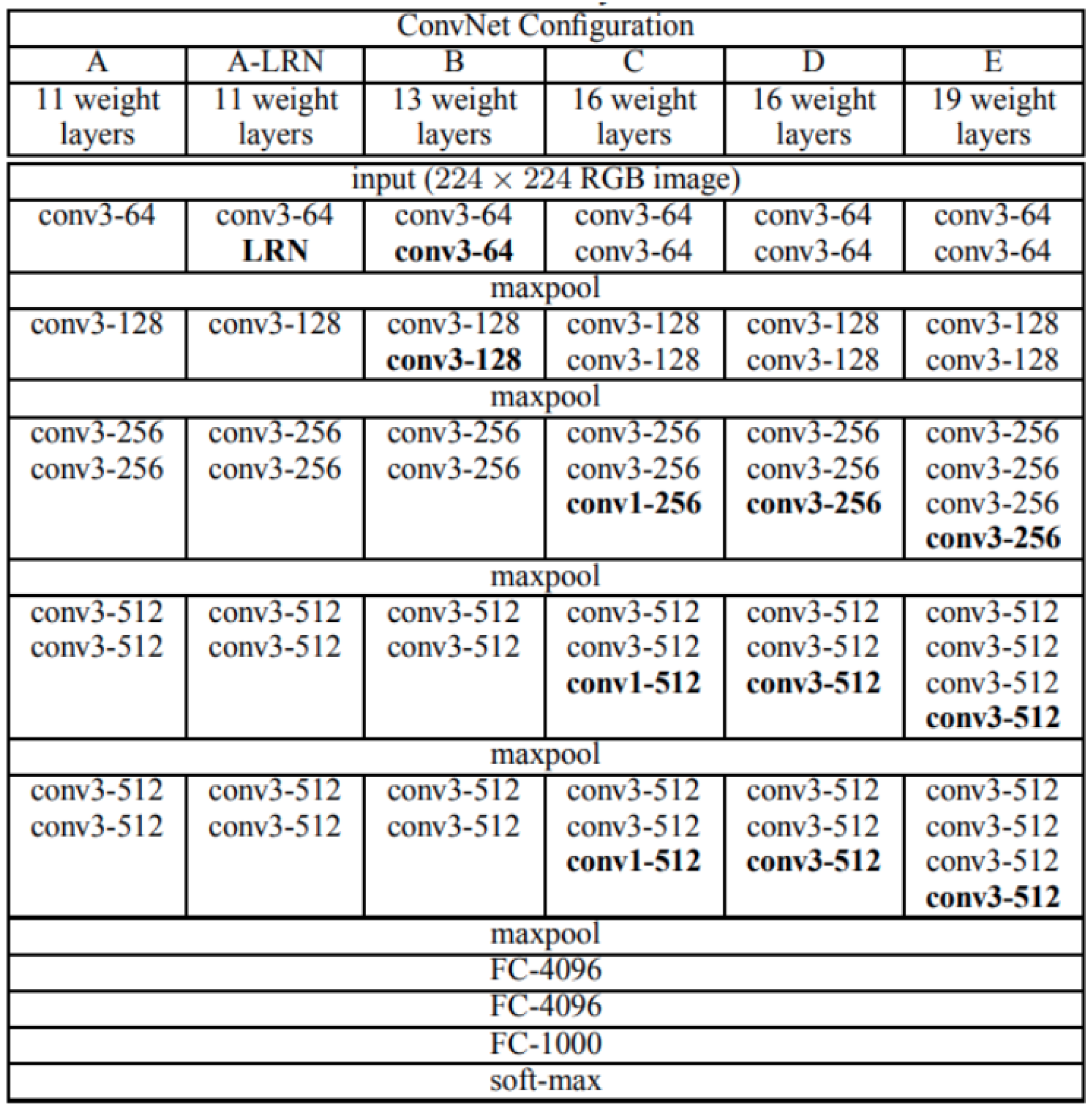
2.2.5. VGGNet
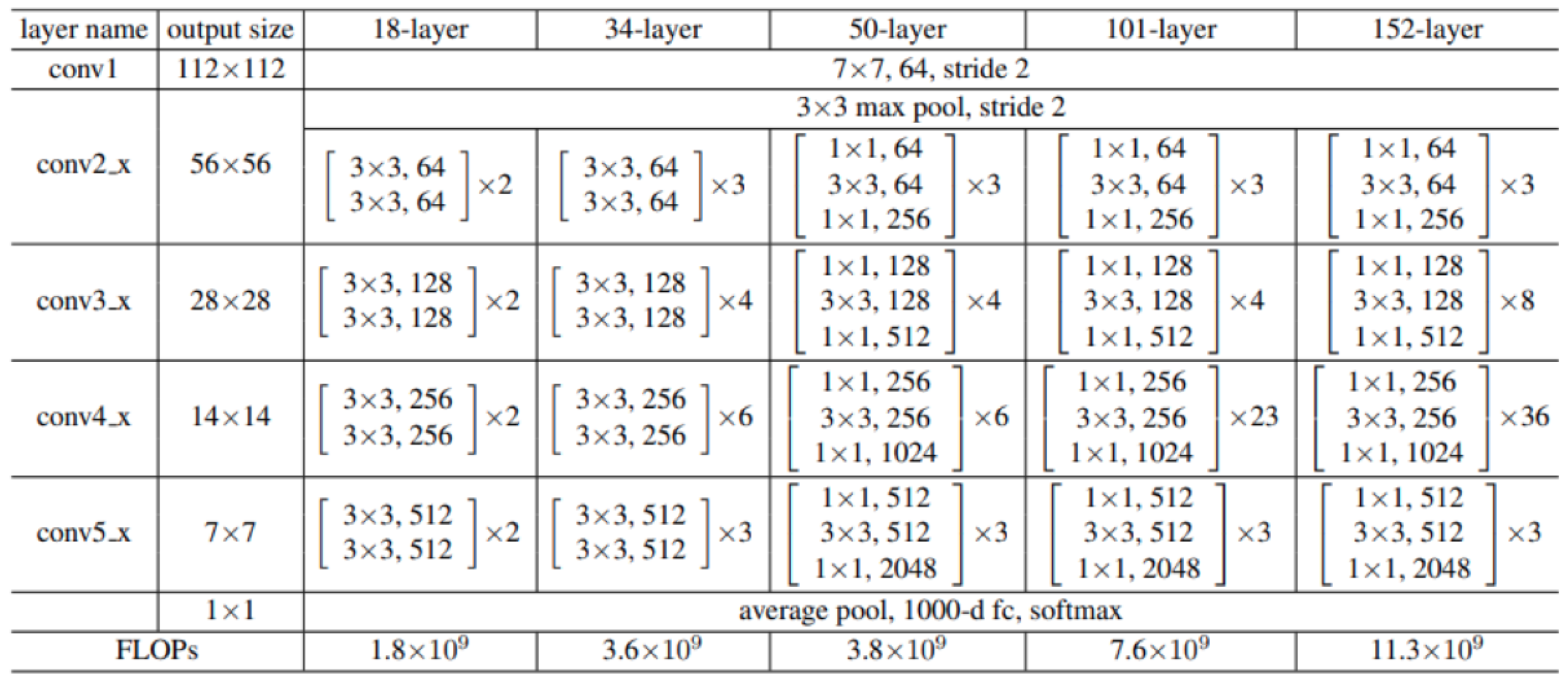
2.2.6. ResNet
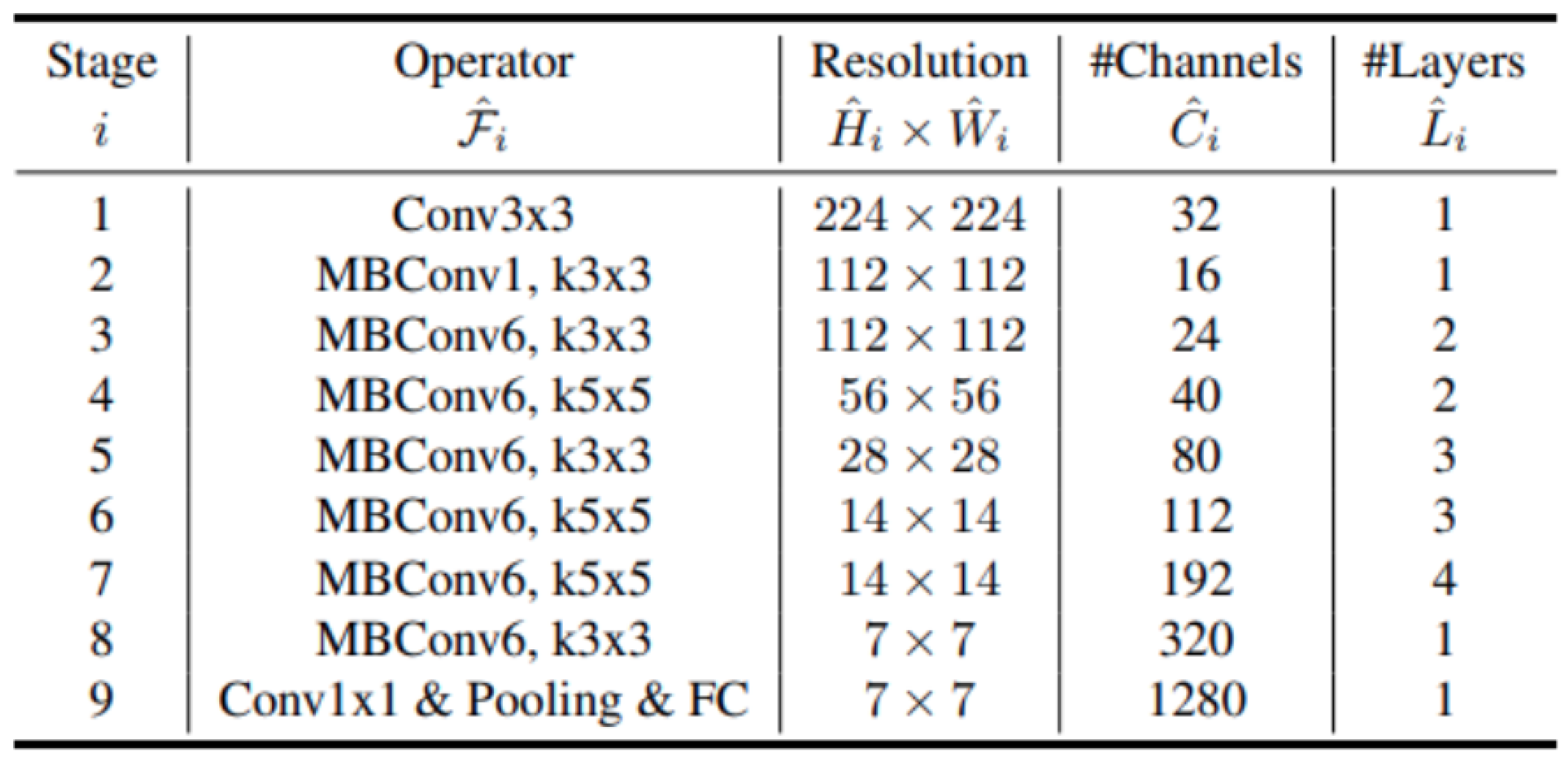
2.2.7. EfficientNet
2.3. Ensemble Classification
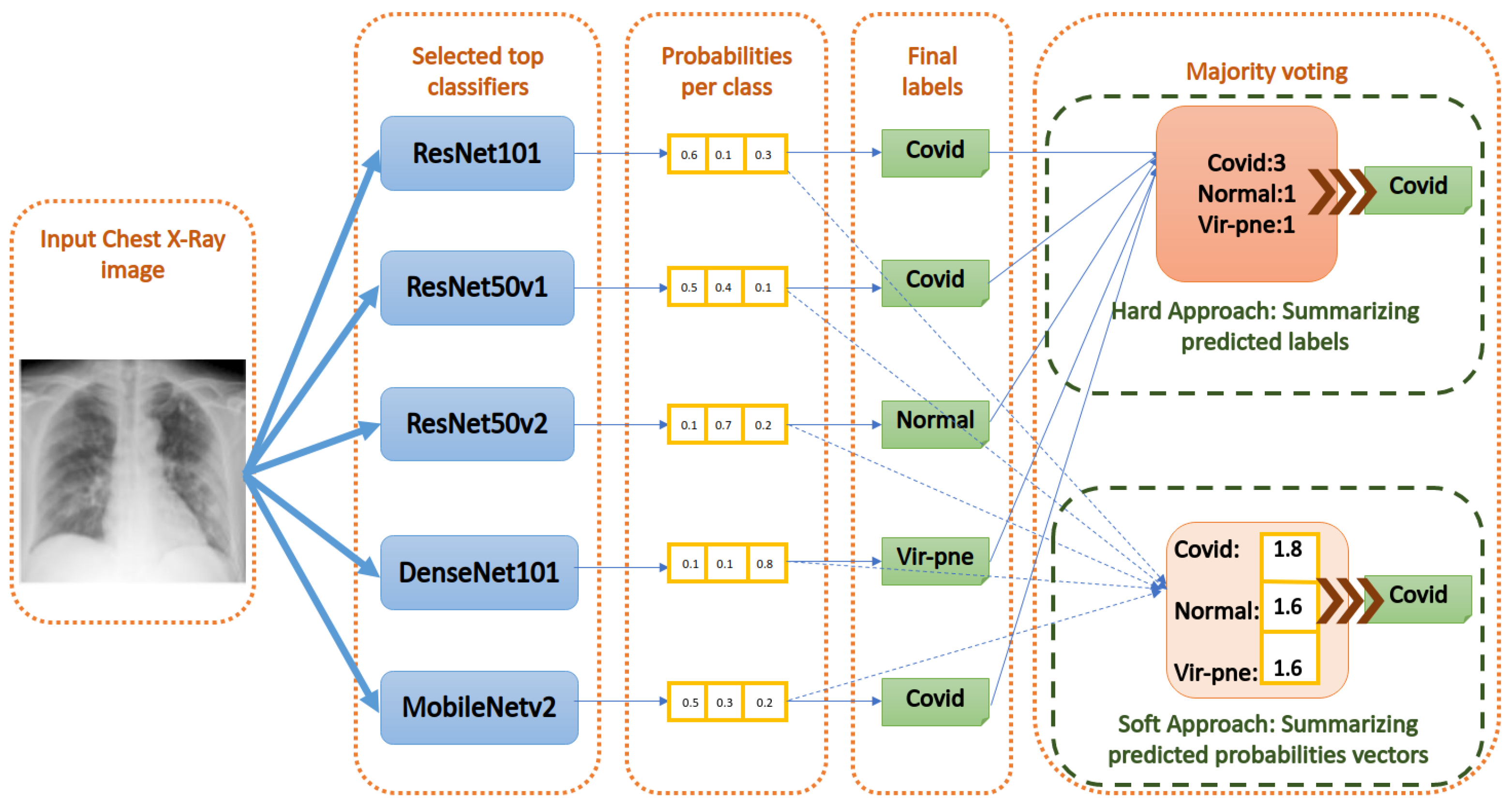
- Majority Voting using the hard approach: As shown in Figure 10, this method acts by summing the per class labels associated with every classifier for the input image. Then, it gives the final label to the class that has the greatest number of labels (votes) among the classifiers. If there are equal votes for two different classes, we chose to assign the final label to the class with the least index. Other strategies can be used to solve this special case, as well.
- Majority Voting using the soft approach: As shown in Figure 10, this method acts by summing the per class values of the probability vector generated by every classifier for the input image. Then, it gives the final label to the class that has the greatest probability sum. Equal probabilities sum is an almost impossible case for the soft approach.
- Weighted voting using a Neural Network: Here, we designed a more dedicated voting approach in order to give a learned weight for every classifier prediction. In fact, manually giving a weight for every classifier is not practical. To solve this problem, we decided to assign the weights using a Neural Network. The Neural Network is trained on the validation set and tested on the test set. In the end, every classifier will be assigned a conditional weight that depends on other classifiers to deduce the most accurate label for the input image.
- SVM (Support vector machine)-based voting: To deduce the right classification of the input image, an SVM is trained to deduce the right classification of the input image by only seeing the vector of labels assigned by the top classifiers. The training of the SVM is made on the validation set and tested on the test set.
- Random Forests-based voting: The Random Forests algorithm acts by building a number of decision trees during the training and generating as output the mode of the assigned classes by the individual trees. The Random Forests method has the advantage of avoiding the habit of overfitting for the normal decision tree. Here, we do the same; many decision trees are built to estimate the right label based on the labels made by the classifiers. Then, we deduce the mode of the estimations made by these decision trees. This mode will be chosen as the final label assigned to the input image.
3. Results
3.1. Experimental Setup
3.2. Performance Evaluation and Metrics
- True Positives (TP): It represents the number of images belonging to a class “X,” and the model predicts correctly that they belong to the class “X”. For example, the input image is of class “Normal” and the model predicts correctly that it is of class “Normal”.
- True Negatives (TN): It represents the number of images that do not belong to a class “X” and the model predicts correctly that they do not belong to the class “X”. For example, the input image is not “COVID”, and the model predicts correctly that it is not of the class “COVID”.
- False Positives (FP): It represents the number of images belonging to a class “X” and the model falsely predicts that it belongs to another class different from “X”. For example, the input image is “COVID” and the model falsely predicts it as “Normal”.
- False Negatives (FN): It represents the number of images that do not belong to a class “X” and the model falsely predicts that they belong to the class “X”. For example, the input image is not “COVID”, and the model predicts it falsely as “COVID”.
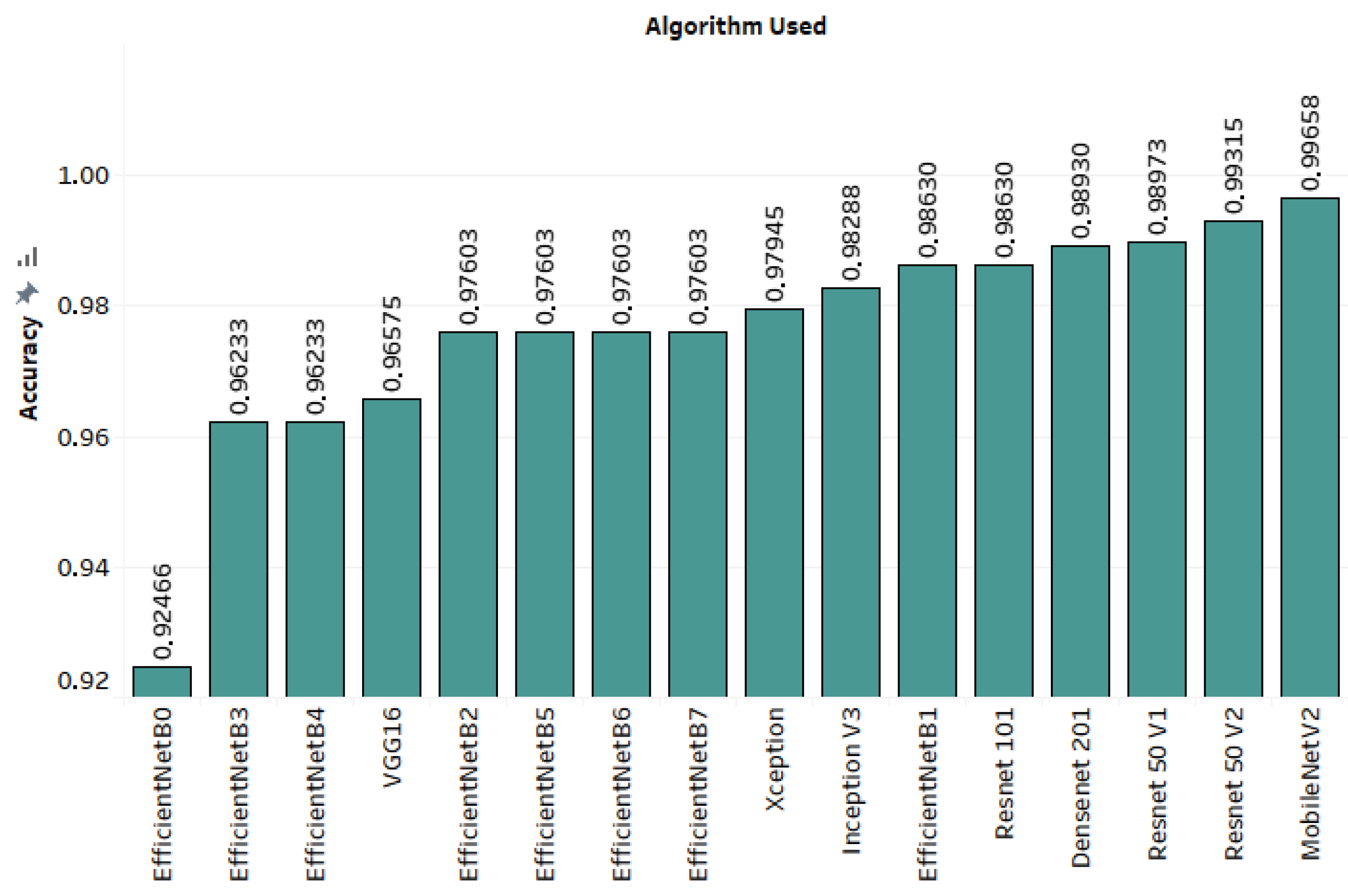
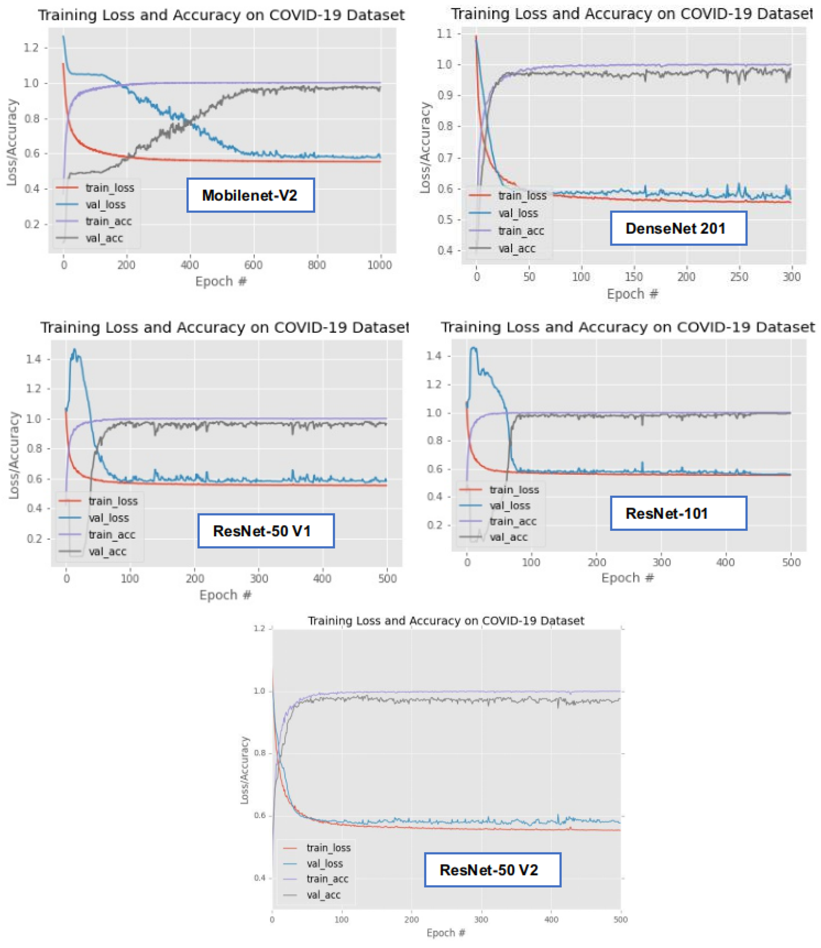
3.3. Results
3.4. Ensemble Voting Appraoches
3.5. Discussion
4. Conclusions
Author Contributions
Funding
Data Availability Statement
Acknowledgments
Conflicts of Interest
References
- Goodfellow, I.; Bengio, Y.; Courville, A. Deep Learning; MIT Press: Cambridge, MA, USA, 2016. [Google Scholar]
- Koubâa, A.; Ammar, A.; Benjdira, B.; Al-Hadid, A.; Kawaf, B.; Al-Yahri, S.A.; Babiker, A.; Assaf, K.; Ras, M.B. Activity Monitoring of Islamic Prayer (Salat) Postures using Deep Learning. In Proceedings of the 2020 6th Conference on Data Science and Machine Learning Applications (CDMA), Riyadh, Saudi Arabia, 4–5 March 2020; pp. 106–111. [Google Scholar]
- Benjdira, B.; Ouni, K.; Al Rahhal, M.M.; Albakr, A.; Al-Habib, A.; Mahrous, E. Spinal Cord Segmentation in Ultrasound Medical Imagery. Appl. Sci. 2020, 10, 1370. [Google Scholar] [CrossRef] [Green Version]
- Benjdira, B.; Ammar, A.; Koubaa, A.; Ouni, K. Data-Efficient Domain Adaptation for Semantic Segmentation of Aerial Imagery Using Generative Adversarial Networks. Appl. Sci. 2020, 10, 1092. [Google Scholar] [CrossRef] [Green Version]
- Benjdira, B.; Bazi, Y.; Koubaa, A.; Ouni, K. Unsupervised Domain Adaptation Using Generative Adversarial Networks for Semantic Segmentation of Aerial Images. Remote Sens. 2019, 11, 1369. [Google Scholar] [CrossRef] [Green Version]
- Alhichri, H.; Bazi, Y.; Alajlan, N.; Bin Jdira, B. Helping the Visually Impaired See via Image Multi-labeling Based on SqueezeNet CNN. Appl. Sci. 2019, 9, 4656. [Google Scholar] [CrossRef] [Green Version]
- Alhichri, H.; Jdira, B.B.; Alajlan, N. Multiple Object Scene Description for the Visually Impaired Using Pre-trained Convolutional Neural Networks. In International Conference on Image Analysis and Recognition; Springer: Berlin/Heidelberg, Germany, 2016; pp. 290–295. [Google Scholar]
- Koubaa, A. Understanding the covid19 outbreak: A comparative data analytics and study. arXiv 2020, arXiv:2003.14150. [Google Scholar]
- Corman, V.M.; Landt, O.; Kaiser, M.; Molenkamp, R.; Meijer, A.; Chu, D.K.; Bleicker, T.; Brünink, S.; Schneider, J.; Schmidt, M.L.; et al. Detection of 2019 novel coronavirus (2019-nCoV) by real-time RT-PCR. Eurosurveillance 2020, 25, 2000045. [Google Scholar] [CrossRef] [PubMed] [Green Version]
- Huang, C.; Wang, Y.; Li, X.; Ren, L.; Zhao, J.; Hu, Y.; Zhang, L.; Fan, G.; Xu, J.; Gu, X.; et al. Clinical features of patients infected with 2019 novel coronavirus in Wuhan, China. Lancet 2020, 395, 497–506. [Google Scholar] [CrossRef] [Green Version]
- Xu, X.; Jiang, X.; Ma, C.; Du, P.; Li, X.; Lv, S.; Yu, L.; Chen, Y.; Su, J.; Lang, G.; et al. Deep learning system to screen coronavirus disease 2019 pneumonia. arXiv 2020, arXiv:2002.09334. [Google Scholar] [CrossRef]
- Shan, F.; Gao, Y.; Wang, J.; Shi, W.; Shi, N.; Han, M.; Xue, Z.; Shen, D.; Shi, Y. Lung infection quantification of covid-19 in ct images with deep learning. arXiv 2020, arXiv:2003.04655. [Google Scholar]
- Xie, X.; Zhong, Z.; Zhao, W.; Zheng, C.; Wang, F.; Liu, J. Chest CT for typical 2019-nCoV pneumonia: Relationship to negative RT-PCR testing. Radiology 2020, 296. [Google Scholar] [CrossRef] [Green Version]
- Ucar, F.; Korkmaz, D. COVIDiagnosis-Net: Deep Bayes-SqueezeNet based Diagnostic of the Coronavirus Disease 2019 (COVID-19) from X-ray Images. Med. Hypotheses 2020, 140, 109761. [Google Scholar] [CrossRef]
- Wang, W.; Xu, Y.; Gao, R.; Lu, R.; Han, K.; Wu, G.; Tan, W. Detection of SARS-CoV-2 in different types of clinical specimens. Jama 2020, 323, 1843–1844. [Google Scholar] [CrossRef] [Green Version]
- Wang, L.; Wong, A. COVID-Net: A tailored deep convolutional neural network design for detection of COVID-19 cases from chest radiography images. arXiv 2020, arXiv:2003.09871. [Google Scholar] [CrossRef]
- Duran-Lopez, L.; Dominguez-Morales, J.P.; Corral-Jaime, J.; Vicente-Diaz, S.; Linares-Barranco, A. COVID-XNet: A custom deep learning system to diagnose and locate COVID-19 in chest X-ray images. Appl. Sci. 2020, 10, 5683. [Google Scholar] [CrossRef]
- Sahlol, A.T.; Yousri, D.; Ewees, A.A.; Al-Qaness, M.A.; Damasevicius, R.; Abd Elaziz, M. COVID-19 image classification using deep features and fractional-order marine predators algorithm. Sci. Rep. 2020, 10, 1–15. [Google Scholar] [CrossRef] [PubMed]
- Szegedy, C.; Vanhoucke, V.; Ioffe, S.; Shlens, J.; Wojna, Z. Rethinking the inception architecture for computer vision. In Proceedings of the IEEE Conference on Computer Vision and Pattern Recognition, Las Vegas, NV, USA, 26 June–1 July 2016; pp. 2818–2826. [Google Scholar]
- Faramarzi, A.; Heidarinejad, M.; Mirjalili, S.; Gandomi, A.H. Marine Predators Algorithm: A nature-inspired metaheuristic. Expert Syst. Appl. 2020, 152, 113377. [Google Scholar] [CrossRef]
- Chowdhury, M.E.; Rahman, T.; Khandakar, A.; Mazhar, R.; Kadir, M.A.; Mahbub, Z.B.; Islam, K.R.; Khan, M.S.; Iqbal, A.; Al-Emadi, N.; et al. Can AI help in screening Viral and COVID-19 pneumonia? arXiv 2020, arXiv:2003.13145. [Google Scholar]
- Karakanis, S.; Leontidis, G. Lightweight deep learning models for detecting COVID-19 from chest X-ray images. Comput. Biol. Med. 2021, 130, 104181. [Google Scholar] [CrossRef] [PubMed]
- Mirza, M.; Osindero, S. Conditional generative adversarial nets. arXiv 2014, arXiv:1411.1784. [Google Scholar]
- Cohen, J.P.; Morrison, P.; Dao, L.; Roth, K.; Duong, T.Q.; Ghassemi, M. Covid-19 image data collection: Prospective predictions are the future. arXiv 2020, arXiv:2006.11988. [Google Scholar]
- Chest X-Ray Images (Pneumonia). Available online: https://www.kaggle.com/paultimothymooney/chest-xray-pneumonia (accessed on 2 March 2021).
- Zebin, T.; Rezvy, S. COVID-19 detection and disease progression visualization: Deep learning on chest X-rays for classification and coarse localization. Appl. Intell. 2021, 51, 1010–1021. [Google Scholar] [CrossRef]
- Zhu, J.Y.; Park, T.; Isola, P.; Efros, A.A. Unpaired image-to-image translation using cycle-consistent adversarial networks. In Proceedings of the IEEE International Conference on Computer Vision, Venice, Italy, 22–29 October 2017; pp. 2223–2232. [Google Scholar]
- Tan, M.; Le, Q.V. Efficientnet: Rethinking model scaling for convolutional neural networks. arXiv 2019, arXiv:1905.11946. [Google Scholar]
- Farooq, M.; Hafeez, A. Covid-resnet: A deep learning framework for screening of covid19 from radiographs. arXiv 2020, arXiv:2003.14395. [Google Scholar]
- Ng, M.Y.; Lee, E.Y.; Yang, J.; Yang, F.; Li, X.; Wang, H.; Lui, M.M.S.; Lo, C.S.Y.; Leung, B.; Khong, P.L.; et al. Imaging profile of the COVID-19 infection: Radiologic findings and literature review. Radiol. Cardiothorac. Imaging 2020, 2, e200034. [Google Scholar] [CrossRef] [Green Version]
- Deng, J.; Dong, W.; Socher, R.; Li, L.J.; Li, K.; Fei-Fei, L. Imagenet: A large-scale hierarchical image database. In Proceedings of the 2009 IEEE Conference on Computer Vision and Pattern Recognition, Miami, FL, USA, 20–25 June 2009; pp. 248–255. [Google Scholar]
- Howard, J.; Gugger, S. Fastai: A layered API for deep learning. Information 2020, 11, 108. [Google Scholar] [CrossRef] [Green Version]
- Minaee, S.; Kafieh, R.; Sonka, M.; Yazdani, S.; Soufi, G.J. Deep-covid: Predicting covid-19 from chest x-ray images using deep transfer learning. arXiv 2020, arXiv:2004.09363. [Google Scholar] [CrossRef] [PubMed]
- Sandler, M.; Howard, A.; Zhu, M.; Zhmoginov, A.; Chen, L.C. Mobilenetv2: Inverted residuals and linear bottlenecks. In Proceedings of the IEEE Conference on Computer Vision and Pattern Recognition, Salt Lake City, UT, USA, 18–22 June 2018; pp. 4510–4520. [Google Scholar]
- Chollet, F. Xception: Deep learning with depthwise separable convolutions. In Proceedings of the IEEE Conference on Computer Vision and Pattern Recognition, Honolulu, HI, USA, 21–26 July 2017; pp. 1251–1258. [Google Scholar]
- Huang, G.; Liu, Z.; Van Der Maaten, L.; Weinberger, K.Q. Densely connected convolutional networks. In Proceedings of the IEEE Conference on Computer Vision and Pattern Recognition, Honolulu, HI, USA, 21–26 July 2017; pp. 4700–4708. [Google Scholar]
- Qassim, H.; Feinzimer, D.; Verma, A. Residual squeeze vgg16. arXiv 2017, arXiv:1705.03004. [Google Scholar]
- He, K.; Zhang, X.; Ren, S.; Sun, J. Deep residual learning for image recognition. In Proceedings of the IEEE Conference on Computer Vision and Pattern Recognition, Las Vegas, NV, USA, 26 June–1 July 2016; pp. 770–778. [Google Scholar]
- Khan, A.; Sohail, A.; Zahoora, U.; Qureshi, A.S. A survey of the recent architectures of deep convolutional neural networks. Artif. Intell. Rev. 2020, 53, 5455–5516. [Google Scholar] [CrossRef] [Green Version]
- Google. Advanced Guide to Inception v3 on Cloud TPU. Available online: https://cloud.google.com/tpu/docs/inception-v3-advanced?hl=en (accessed on 3 March 2021).
- Simonyan, K.; Zisserman, A. Very Deep Convolutional Networks for Large-Scale Image Recognition. arXiv 2014, arXiv:1409.1556. [Google Scholar]
- Al-Mukhtar, M. Random forest, support vector machine, and neural networks to modelling suspended sediment in Tigris River-Baghdad. Environ. Monit. Assess. 2019, 191, 1–12. [Google Scholar] [CrossRef]
- Han, T.; Jiang, D.; Zhao, Q.; Wang, L.; Yin, K. Comparison of random forest, artificial neural networks and support vector machine for intelligent diagnosis of rotating machinery. Trans. Inst. Meas. Control 2018, 40, 2681–2693. [Google Scholar] [CrossRef]
- Liu, M.; Wang, M.; Wang, J.; Li, D. Comparison of random forest, support vector machine and back propagation neural network for electronic tongue data classification: Application to the recognition of orange beverage and Chinese vinegar. Sens. Actuators B Chem. 2013, 177, 970–980. [Google Scholar] [CrossRef]
- Raczko, E.; Zagajewski, B. Comparison of support vector machine, random forest and neural network classifiers for tree species classification on airborne hyperspectral APEX images. Eur. J. Remote Sens. 2017, 50, 144–154. [Google Scholar] [CrossRef] [Green Version]
- Nitze, I.; Schulthess, U.; Asche, H. Comparison of machine learning algorithms random forest, artificial neural network and support vector machine to maximum likelihood for supervised crop type classification. In Proceedings of the 4th GEOBIA, Rio de Janeiro, Brazil, 7–9 May 2012; Volume 35. [Google Scholar]
- Martinez-Castillo, C.; Astray, G.; Mejuto, J.C.; Simal-Gandara, J. Random forest, artificial neural network, and support vector machine models for honey classification. eFood 2019, 1, 69–76. [Google Scholar] [CrossRef] [Green Version]
- Abadi, M.; Barham, P.; Chen, J.; Chen, Z.; Davis, A.; Dean, J.; Devin, M.; Ghemawat, S.; Irving, G.; Isard, M.; et al. TensorFlow: A system for large-scale machine learning. arXiv 2016, arXiv:1605.08695. [Google Scholar]
- Chollet, F. Keras. 2015. Available online: https://github.com/fchollet/keras (accessed on 21 March 2021).
- Pedregosa, F.; Varoquaux, G.; Gramfort, A.; Michel, V.; Thirion, B.; Grisel, O.; Blondel, M.; Müller, A.; Nothman, J.; Louppe, G.; et al. Scikit-learn: Machine Learning in Python. arXiv 2012, arXiv:1201.0490. [Google Scholar]
- Van Rossum, G.; Drake, F.L., Jr. Python Tutorial; Centrum voor Wiskunde en Informatica: Amsterdam, The Netherlands, 1995. [Google Scholar]
- Jupyter Lab Project. Available online: https://jupyter.org/ (accessed on 4 March 2021).
- Fisher, R.A. The Design of Experiments; Oliver & Boyd: Edinburgh, UK, 1937. [Google Scholar]


| Ref. | Dataset Used | Algorithms | Main Results | |||
|---|---|---|---|---|---|---|
| Accuracy | Recall | Precision | ||||
| 1 [11] | A total of 618 CT samples: 219 CT samples with COVID-19; 224 CT samples with Influenza-A viral pneumonia; and 175 CT samples from healthy people. 528 CT samples for training 90 CT samples for validation | 3D CNN model based on the classical ResNet18 network structure. | Normal | 86.7% | 90.0% | 93.1% |
| Non-COVID-19 | 83.3% | 86.2% | ||||
| COVID-19 | 86.7% | 81.3% | ||||
| 2 [12] | 300 CT images of COVID-19 cases for validation. 249 CT images of COVID-19 cases for training. | The “VB Net” model is a combination between the V-Net model and the bottleneck model for automatic segmentation and quantification | Normal | 91.6% | - | - |
| Non-COVID-19 | - | - | ||||
| COVID-19 | - | - | ||||
| 3 [16] | COVIDx dataset: 16,756 chest-X-ray images from 13,645 patient cases: 76 images from 53 COVID-19 patient cases, 8066 patient normal cases, 5526 patient non-COVID-19 pneumonia cases | The COVID-Net network architecture uses a lightweight residual (PEPX) design pattern. | Normal | 93.3% | 95.0% | 90.5% |
| Non-COVID-19 | 94.0% | 91.3% | ||||
| COVID-19 | 91.0% | 98.9% | ||||
| 4 [29] | A total of 5941 posteroanterior chest-X-ray images from 2839 patients: 68 COVID-19 images from45 COVID-19 patients. 1203 patients with Normal class, 931 patients with a bacterial pneumonia 660 patients with non-COVID-19 viral pneumonia cases. | The ResNet50 model for classification. | Normal | 96.2% | 96.5% | 99.1% |
| Non-COVID-19 | 93.9% | 92.7% | ||||
| COVID-19 | 100.0% | 100.0% | ||||
| 5 [33] | COVID-X-ray-5k: It contains 2084 training and 3100 test images. - 2084 images for training divided into 84 COVID-19 and 2000 Non-COVID - 3100 images for testing divided into 100 COVID-19 and 3000 Non-COVID. | 4 CNN models, including ResNet18, ResNet50, SqueezeNet, and DenseNet-121, to identify COVID-19 disease in the analyzed chest X-ray images. | Normal | 89.5% | - | - |
| Non-COVID-19 | - | - | ||||
| COVID-19 | - | - | ||||
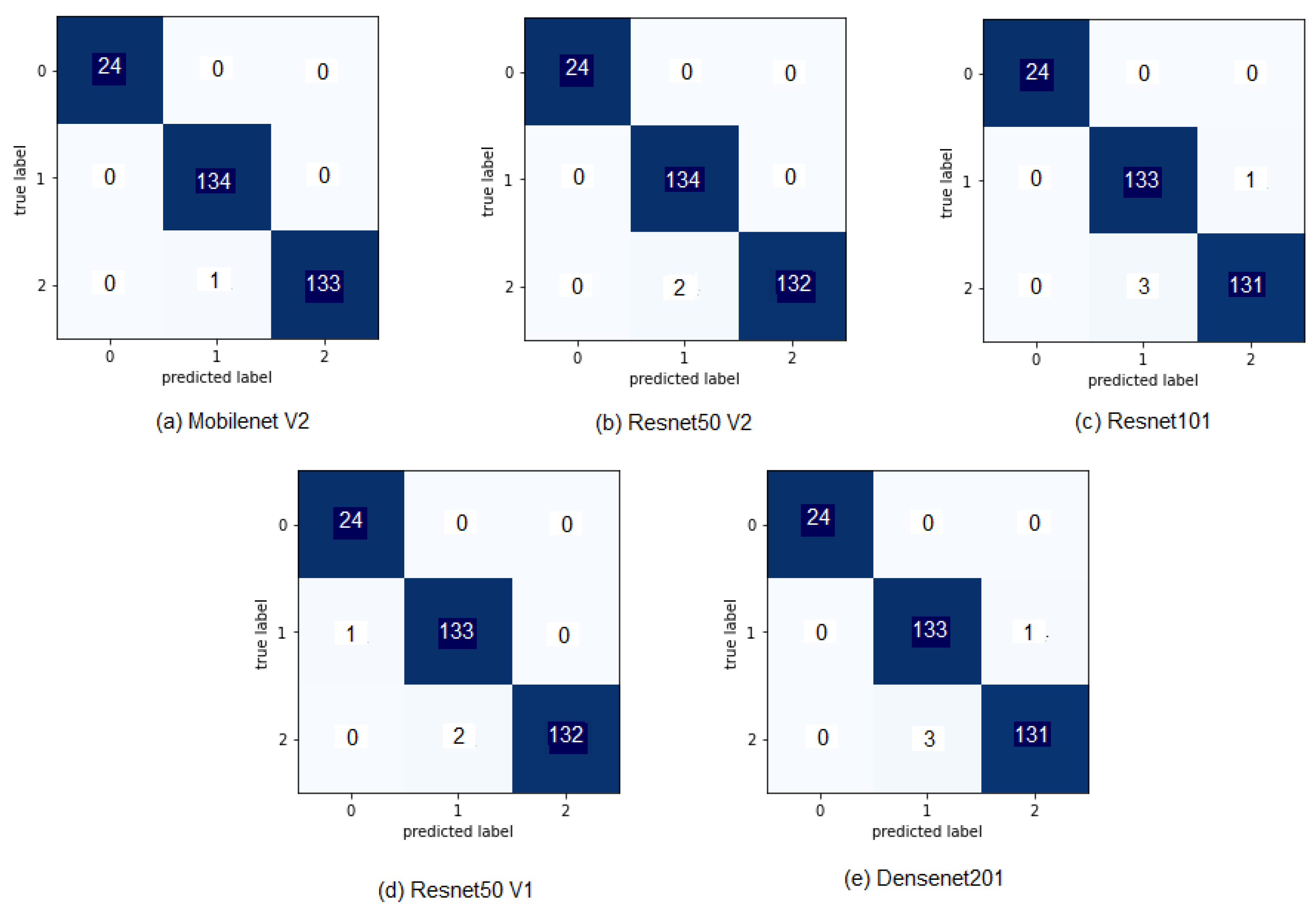
| Our paper | The chest X-ray dataset contains 2911 images divided into: 237 COVID-19 positive images, 1338 normal images, 1336 viral pneumonia images. 2328 images for the training, 291 images for the validation, 292 images for testing. | MobileNet-V2, Xception, Inception-V3, DenseNet-201, VGG16, Resnet-50 (V1 and V2), Resnet 101, and EfficientNet (B0, B1, B2, B3, B4, B5, B6, and B7), and Ensemble classification using voting. | Normal | 99.31% | 100.0% | 98.52% |
| Non-COVID-19 | 98.50% | 100.0% | ||||
| COVID-19 | 100.0% | 100.0% | ||||
| Model | Learning Rate | Batch Size | Epochs Number of Best Convergence | Number of Epochs |
|---|---|---|---|---|
| MobileNetV2 | 1.00 × 10⁻⁵ | 200 | 760 | 1000 |
| Xception | 1.00 × 10⁻⁵ | 100 | 471 | 500 |
| InceptionV3 | 1.00 × 10⁻⁵ | 100 | 369 | 400 |
| DenseNet-201 | 1.00 × 10⁻⁵ | 64 | 270 | 300 |
| VGG16 | 1.00 × 10⁻⁴ | 64 | 169 | 200 |
| ResNet50V1 | 1.00 × 10⁻⁵ | 100 | 152 | 200 |
| ResNet50V2 | 1.00 × 10⁻⁵ | 100 | 231 | 300 |
| ResNet11 | 1.00 × 10⁻⁵ | 100 | 425 | 500 |
| EfficientNet-B0 | 1.00 × 10⁻⁴ | 32 | 224 | 300 |
| EfficientNet-B1 | 1.00 × 10⁻⁵ | 32 | 152 | 200 |
| EfficientNet-B2 | 1.00 × 10⁻⁵ | 32 | 280 | 300 |
| EfficientNet-B3 | 1.00 × 10⁻⁵ | 32 | 373 | 400 |
| EfficientNet-B4 | 1.00 × 10⁻⁵ | 32 | 350 | 400 |
| EfficientNet-B5 | 1.00 × 10⁻⁵ | 32 | 415 | 500 |
| EfficientNet-B6 | 1.00 × 10⁻⁵ | 16 | 252 | 300 |
| EfficientNet-B7 | 1.00 × 10⁻⁵ | 16 | 290 | 300 |
| ALGORITHM USED | Accuracy | Precision | Recall | F1-Score |
|---|---|---|---|---|
| EfficientNet-B0 | 0.9549 | 0.66197 | 0.93925 | 0.79325 |
| EfficientNet-B6 | 0.97466 | 0.84821 | 1 | 0.91787 |
| EfficientNet-B2 | 0.98969 | 0.89623 | 1 | 0.94527 |
| EfficientNet-B4 | 0.99012 | 0.96447 | 1 | 0.98191 |
| EfficientNet-B3 | 0.99527 | 0.96447 | 1 | 0.98191 |
| EfficientNet-B5 | 0.99871 | 1 | 1 | 1 |
| VGG16 | 0.99914 | 1 | 1 | 1 |
| EfficientNet-B1 | 0.99957 | 1 | 1 | 1 |
| ResNet50V2 | 0.99957 | 1 | 1 | 1 |
| DenseNet-201 | 0.99957 | 1 | 1 | 1 |
| Xception | 0.99957 | 1 | 0.99474 | 0.99736 |
| MobileNetV2 | 1 | 1 | 1 | 1 |
| InceptionV3 | 1 | 1 | 1 | 1 |
| ResNet50V1 | 1 | 1 | 1 | 1 |
| ResNet11 | 1 | 1 | 1 | 1 |
| EfficientNet-B7 | 1 | 1 | 1 | 1 |
| Mean | 0.99379 | 0.95845 | 0.99587 | 0.97609 |
| SD | 0.01235 | 0.09054 | 0.01515 | 0.05416 |
| Confidence Level (95.0%) | 0.00658 | 0.04825 | 0.00807 | 0.02886 |
| Confidence Interval (95.0%) | 0.98721–1 | 0.91020–1 | 0.98779–1 | 0.94723–1 |
| ALGORITHM USED | Accuracy | Precision | Recall | F1-Score |
|---|---|---|---|---|
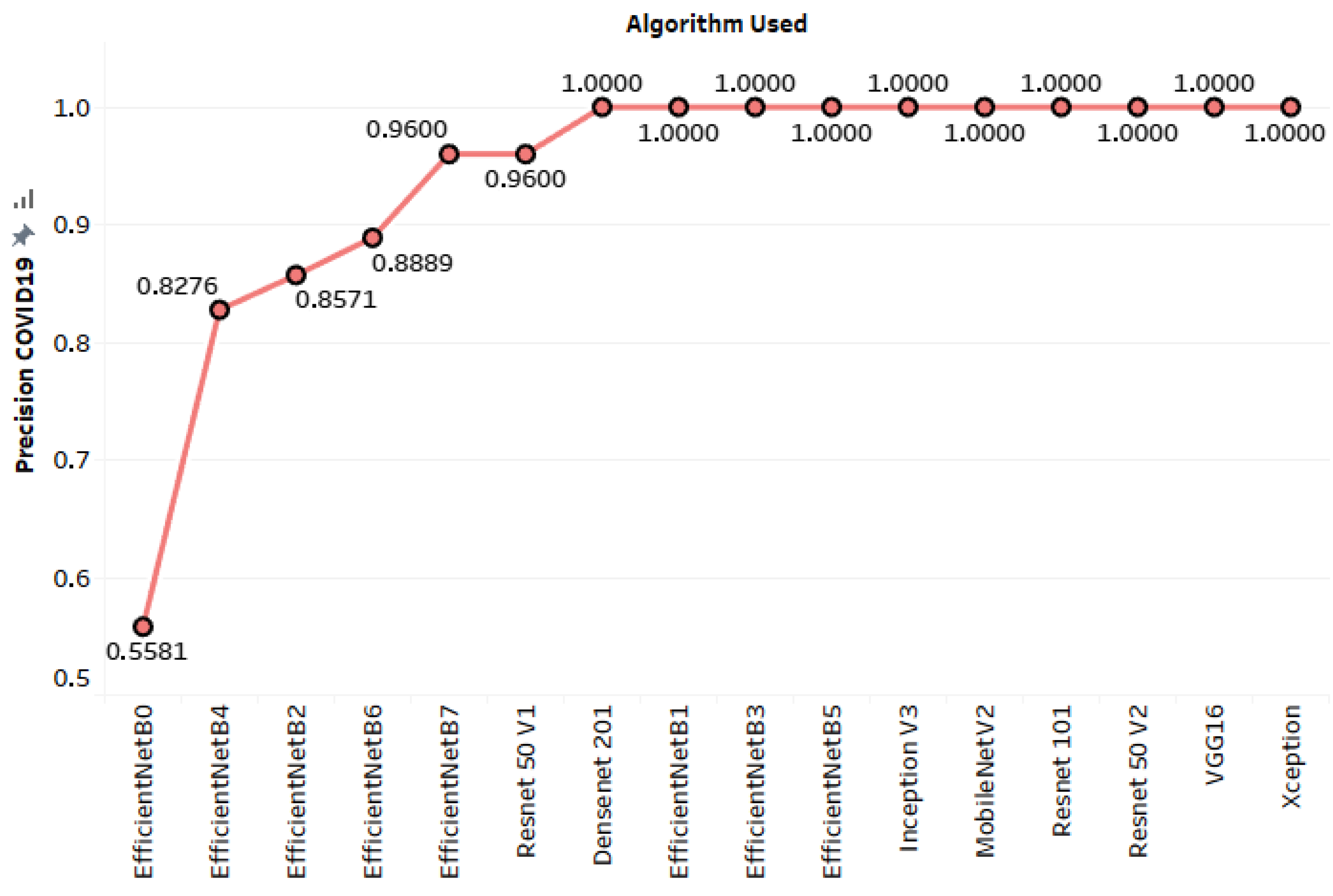
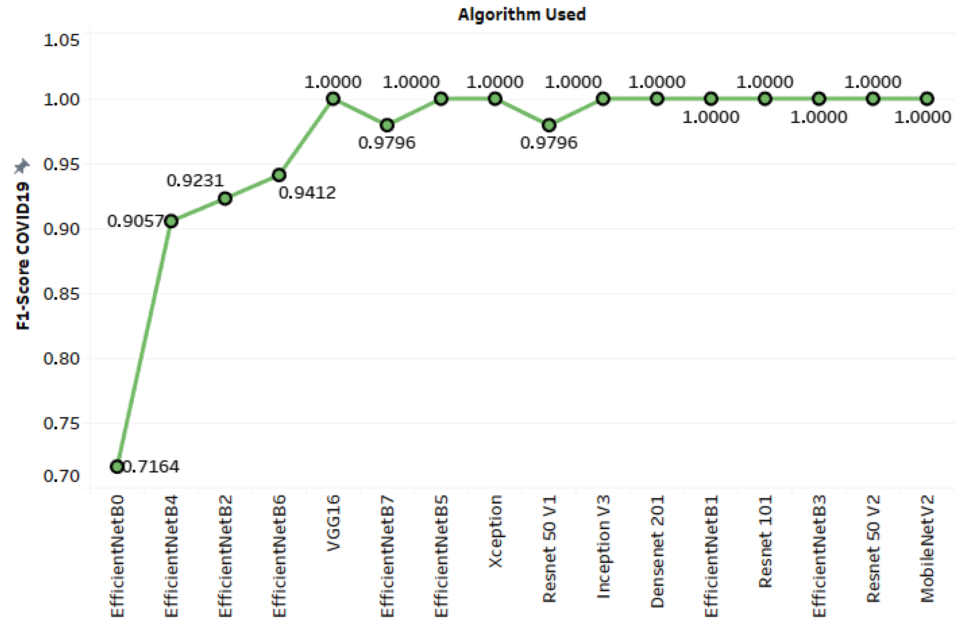
| EfficientNet-B0 | 0.92466 | 0.55814 | 1 | 0.71642 |
| EfficientNet-B3 | 0.96233 | 0.82759 | 1 | 0.90566 |
| EfficientNet-B4 | 0.96233 | 0.82759 | 1 | 0.90566 |
| VGG16 | 0.96575 | 1 | 1 | 1 |
| EfficientNet-B2 | 0.97603 | 0.85714 | 1 | 0.92308 |
| EfficientNet-B5 | 0.97603 | 1 | 1 | 1 |
| EfficientNet-B6 | 0.97603 | 0.88889 | 1 | 0.94118 |
| EfficientNet-B7 | 0.97603 | 0.96 | 1 | 0.97959 |
| Xception | 0.97945 | 1 | 1 | 1 |
| InceptionV3 | 0.98288 | 1 | 1 | 1 |
| EfficientNet-B1 | 0.9863 | 1 | 1 | 1 |
| ResNet11 | 0.9863 | 1 | 1 | 1 |
| DenseNet-201 | 0.9893 | 1 | 1 | 1 |
| ResNet50V1 | 0.98973 | 0.96 | 1 | 0.97959 |
| ResNet50V2 | 0.99315 | 1 | 1 | 1 |
| MobileNetV2 | 0.99658 | 1 | 1 | 1 |
| Majority Voting (hard approach) | 0.99315 | 1 | 1 | 1 |
| Majority Voting (soft approach) | 0.99315 | 1 | 1 | 1 |
| Weighted Voting using Neural Networks | 0.98630 | 1 | 1 | 1 |
| SVM-based voting | 0.98973 | 1 | 1 | 1 |
| Random Forests-based voting | 0.98630 | 1 | 1 | 1 |
| Mean | 0.97945 | 0.94663 | 1 | 0.969104 |
| SD | 0.01602 | 0.10743 | 0 | 0.066476 |
| Confidence Level (95.0%) | 0.00729 | 0.048903 | 0 | 0.03026 |
| Confidence Interval (95.0%) | 0.97215–0.98674 | 0.89773–0.99553 | 1–1 | 0.93884–0.99936 |
| ALGORITHM USED | Inference Time (ms) |
|---|---|
| EfficientNet-B0 | 2 |
| EfficientNet-B3 | 2 |
| EfficientNet-B4 | 1 |
| VGG16 | 0.879 |
| EfficientNet-B2 | 2 |
| EfficientNet-B5 | 2 |
| EfficientNet-B6 | 2 |
| EfficientNet-B7 | 2 |
| Xception | 2 |
| InceptionV3 | 1 |
| EfficientNet-B1 | 2 |
| ResNet11 | 0.996 |
| DenseNet-201 | 2 |
| ResNet50V1 | 1 |
| ResNet50V2 | 1 |
| MobileNetV2 | 2 |
| ALGORITHM USED | Accuracy in the Validation Set | Accuracy in the Test Set |
|---|---|---|
| Weighted Voting using Neural Networks | 0.99658 | 0.98630 |
| SVM-based voting | 0.99658 | 0.98973 |
| Random Forests-based voting | 0.99315 | 0.98630 |
| Mean | 0.99543 | 0.98744 |
| SD | 0.00198 | 0.00198 |
| Confidence Level (95.0%) | 0.00491 | 0.00491 |
| Confidence Interval (95.0%) | 0.99051–1 | 0.98252–0.99236 |
| ALGORITHM USED | Accuracy | Precision | Recall | F1-Score |
|---|---|---|---|---|
| EfficientNet-B5 | 0.97603 | 1 | 1 | 1 |
| EfficientNet-B6 | 0.97603 | 0.88889 | 1 | 0.94118 |
| EfficientNet-B7 | 0.97603 | 0.96 | 1 | 0.97959 |
| Majority Voting (hard approach) | 0.98630 | 0.96 | 1 | 0.97959 |
| Majority Voting (soft approach) | 0.98973 | 1 | 1 | 1 |
| Mean | 0.98082 | 0.96177 | 1 | 0.98007 |
| SD | 0.00667 | 0.04538 | 0 | 0.02401 |
| Confidence Level (95.0%) | 0.00828 | 0.05635 | 0 | 0.02982 |
| Confidence Interval (95.0%) | 0.97253–0.98911 | 0.90541–1.00000 | 1–1 | 0.95025–1 |
| AUC Scores Following the OVO Scheme | AUC Scores Following the OVR Scheme | |||
|---|---|---|---|---|
| Macro Average | Prevalence-Weighted Average | Macro Average | Prevalence-Weighted Average | |
| DenseNet-201 | 0.995056 | 0.993194 | 0.995056 | 0.993194 |
| ResNet50V1 | 0.999103 | 0.998765 | 0.999103 | 0.998765 |
| ResNet50V2 | 0.997229 | 0.996185 | 0.997229 | 0.996185 |
| MobileNetV2 | 0.999843 | 0.999783 | 0.999843 | 0.999783 |
| ResNet11 | 0.992285 | 0.989379 | 0.992285 | 0.989379 |
| Soft Majority Voting | 0.999827 | 0.999762 | 0.999827 | 0.999762 |
| Algorithm | Accuracy |
|---|---|
| 3D CNN (ResNet18) [11] | 86.7% |
| VBNet [12] | 91.6% |
| COVID-Net [16] | 93.3% |
| ResNet50 [29] | 96.23% |
| 4 CNN models [33] | 89.5% |
| ResNet50V2 | 99.315% |
| MobileNetV2 | 99.658% |
| Majority Voting | 99.315% |
| ALGORITHM USED | Accuracy | Precision | Recall | F1-Score |
|---|---|---|---|---|
| EfficientNet-B0 | 0.88316 | 0.44681 | 0.91304 | 0.6 |
| EfficientNet-B6 | 0.93471 | 0.6875 | 0.95652 | 0.8 |
| EfficientNet-B4 | 0.94502 | 0.7931 | 1 | 0.88462 |
| EfficientNet-B3 | 0.95189 | 0.82143 | 1 | 0.90196 |
| EfficientNet-B2 | 0.95189 | 0.74194 | 1 | 0.85185 |
| EfficientNet-B1 | 0.95876 | 0.88462 | 1 | 0.93878 |
| InceptionV3 | 0.96564 | 1 | 1 | 1 |
| ResNet50V1 | 0.96564 | 0.88 | 0.95652 | 0.91667 |
| EfficientNet-B5 | 0.96564 | 1 | 1 | 1 |
| VGG16 | 0.96907 | 0.95833 | 1 | 0.97872 |
| ResNet50V2 | 0.97595 | 95652 | 0.95652 | 0.95652 |
| MobileNetV2 | 0.97595 | 0.92 | 1 | 0.95833 |
| Xception | 0.97945 | 1 | 0.95652 | 97778 |
| DenseNet-201 | 0.98625 | 1 | 1 | 1 |
| ResNet11 | 0.99313 | 1 | 1 | 1 |
| EfficientNet-B7 | 0.99313 | 1 | 1 | 1 |
| Majority Voting (hard approach) | 0.99313 | 1 | 1 | 1 |
| Majority Voting (soft approach) | 0.99313 | 1 | 1 | 1 |
| Model | Accuracy on the Test Set | Accuracy on the Validation Set | Average Accuracy |
|---|---|---|---|
| Majority Voting (hard approach) | 0.99315 | 0.99313 | 0.99314 |
| Majority Voting (soft approach) | 0.99315 | 0.99313 | 0.99314 |
| ResNet11 | 0.9863 | 0.99313 | 0.989715 |
| DenseNet-201 | 0.9893 | 0.98625 | 0.987775 |
| MobileNetV2 | 0.99658 | 0.97595 | 0.986265 |
| EfficientNet-B7 | 0.97603 | 0.99313 | 0.98458 |
| ResNet50V2 | 0.99315 | 0.97595 | 0.98455 |
| Xception | 0.97945 | 0.97945 | 0.97945 |
| ResNet50V1 | 0.98973 | 0.96564 | 0.977685 |
| InceptionV3 | 0.98288 | 0.96564 | 0.97426 |
| EfficientNet-B1 | 0.9863 | 0.95876 | 0.97253 |
| EfficientNet-B5 | 0.97603 | 0.96564 | 0.970835 |
| VGG16 | 0.96575 | 0.96907 | 0.96741 |
| EfficientNet-B2 | 0.97603 | 0.95189 | 0.96396 |
| EfficientNet-B3 | 0.96233 | 0.95189 | 0.95711 |
| EfficientNet-B6 | 0.97603 | 0.93471 | 0.95537 |
| EfficientNet-B4 | 0.96233 | 0.94502 | 0.953675 |
| EfficientNet-B0 | 0.92466 | 0.88316 | 0.90391 |
| Model | Test Set | Validation Set |
|---|---|---|
| Majority Voting (hard approach) | 95% | 100% |
| Majority Voting (soft approach) | 95% | 100% |
| ResNet11 | 86% | 100% |
| DenseNet-201 | 90% | 94% |
| MobileNetV2 | 100% | 84% |
| EfficientNet-B7 | 71% | 100% |
| ResNet50V2 | 95% | 84% |
| Xception | 76% | 88% |
| ResNet50V1 | 90% | 75% |
| InceptionV3 | 81% | 75% |
| EfficientNet-B1 | 86% | 69% |
| EfficientNet-B5 | 71% | 75% |
| VGG16 | 57% | 78% |
| EfficientNet-B2 | 71% | 62% |
| EfficientNet-B3 | 52% | 62% |
| EfficientNet-B6 | 71% | 47% |
| EfficientNet-B4 | 52% | 56% |
| EfficientNet-B0 | 0% | 0% |
Publisher’s Note: MDPI stays neutral with regard to jurisdictional claims in published maps and institutional affiliations. |
© 2021 by the authors. Licensee MDPI, Basel, Switzerland. This article is an open access article distributed under the terms and conditions of the Creative Commons Attribution (CC BY) license (http://creativecommons.org/licenses/by/4.0/).
Share and Cite
Ben Jabra, M.; Koubaa, A.; Benjdira, B.; Ammar, A.; Hamam, H. COVID-19 Diagnosis in Chest X-rays Using Deep Learning and Majority Voting. Appl. Sci. 2021, 11, 2884. https://doi.org/10.3390/app11062884
Ben Jabra M, Koubaa A, Benjdira B, Ammar A, Hamam H. COVID-19 Diagnosis in Chest X-rays Using Deep Learning and Majority Voting. Applied Sciences. 2021; 11(6):2884. https://doi.org/10.3390/app11062884
Chicago/Turabian StyleBen Jabra, Marwa, Anis Koubaa, Bilel Benjdira, Adel Ammar, and Habib Hamam. 2021. "COVID-19 Diagnosis in Chest X-rays Using Deep Learning and Majority Voting" Applied Sciences 11, no. 6: 2884. https://doi.org/10.3390/app11062884