Structural Crack Detection and Recognition Based on Deep Learning

Abstract

The detection and recognition of surface cracks are of great significance for structural safety. This paper is based on a deep-learning methodology to detect and recognize structural cracks. First, a training dataset of the model is built. Then, three neural networks, AlexNet, VGGNet13, and ResNet18, are employed to recognize and classify crack images. The tests indicate that the ResNet18 model generates the most satisfactory results. It is also found that the trained YOLOv3 model detects the crack area with satisfactory accuracy. This study also confirms that the proposed deep learning as a novel technology has the potential to be an efficient and robust tool for crack detection and recognition to replace traditional methods.

1. Introduction

Crack damage detection has been a long-standing problem for industrial and civil structures. Traditional crack detection technology comprises both manual and machine detection methods. The manual detection method is generally accepted as less accurate and time consuming. Machine detection technologies have been developed rapidly in recent years using ultrasonic, microwave, or other signals [1,2,3,4,5,6]. Various crack detection approaches exist and can be put into different categories. The first category comprises an excitation device installed at one end of the structural member and a receiving device installed at the other end. By analysing the characteristics of the waveform amplitude and frequency, the location and depth of cracks can be recognized without any destructive damage to the structure. This method, however, has low recognition accuracy. The second category is based on the minimum path algorithm [7,8,9], which considers the image light and geometric characteristics. The path is a series of adjacent pixel values, the sum of the adjacent pixel values indicates the intensity, and the minimum path is a crack. This method requires considerable computational effort. The third method is based on image processing [10,11,12,13,14,15], which implies filtering the collected crack images, such as median filtering and mean filtering, and then using the Hough transform, binarization, and tensor voting to recognize the cracks. The fourth method is based on traditional machine-learning algorithms [16], in which crack pictures are preprocessed using machine-learning algorithms such as random forest and AdaBoost [17]. Another method for crack detection and recognition is based on deep learning [18,19,20,21]. This method is characterized by augmentation of the dataset and the use of convolutional neural networks and segmentation algorithms to recognize, segment, and extract cracks. This method is more accurate and robust than the other categories and is used in this article.

In this paper, we mainly do two things: first, recognize the crack images, and then, perform target detection on the crack area in the crack images. First, three neural networks are utilized to recognize crack images: AlexNet [22], VGGNet13 [23], and ResNet18 [24], and they are compared against each other according to the evaluation indicators. Second, for the classified crack images, it is necessary to detect the crack area. Currently, there are two main detection algorithms commonly used: (i) two-stage methods based on regional recommendations, such as Fast R-CNN [25] and Faster R-CNN [26], and (ii) one-stage methods without regional recommendations, such as SSD [27] and YOLO v3 [28]. Because YOLOv3 has more advantages than other models, such as its faster speed, it is widely used in the industry, especially in scenarios where high precision is not pursued, so the YOLOv3 model is chosen to detect cracks. In this experiment, we found that ResNet18 can accurately recognize crack images, and YOLOv3 can detect the crack area in the video in real time.

2. Experimental Data Preparation

2.1. Image Acquisition

Although there is much research on crack detection in academia, there is no unified crack image dataset. Therefore, to train the crack detection and recognition model, it is necessary to manually collect crack pictures. The data in this experiment are based on camera collection, and the type of cracks targeted is concrete cracks. The camera is used to manually take pictures on roads and bridges to collect crack pictures. A total of 2000 crack pictures were collected, including four types of strong light, moisture, distortion, and darkness. The picture resolution is 1024 × 1024 pixels in the format of JPG.

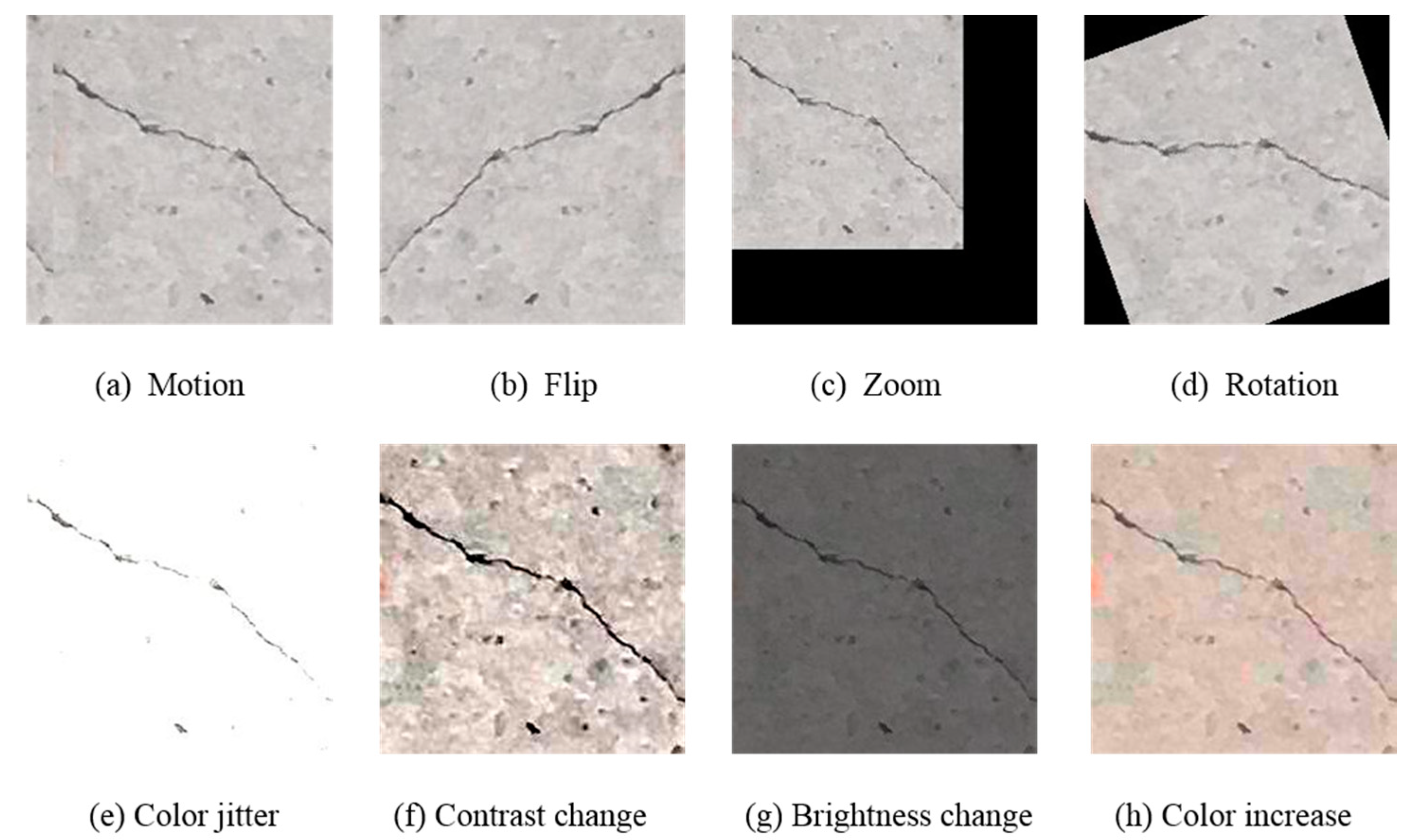
2.2. Crack Recognition Dataset Build

The original collected crack pictures are only 2000. For deep-learning tasks, to obtain a model with good generalization performance and high accuracy, the quantity of data is not enough. The resolution of the original pictures is 1024 × 1024 pixels, and the pixels are large and not suitable for direct input to the neural network. The input image size of the neural network is too large, which will cause too much memory overhead. The number of layers of the neural network is bound to increase. The parameters of the neural network also increase exponentially, which leads to an increase in video memory and training time and a decrease in training batches, making the model show poor performance. To solve the above problems, the experiments were performed with the sliding window cropping technique, which uses 227 × 227 pixel window sliding on the original picture and cropping line by line without overlapping. The resolution of the cropped picture is 227 × 227 pixels. Then, manual classification was performed to obtain a dataset of 10,000 crack pictures and 10,000 background pictures without cracks.

To improve the generalization ability of the model, it is necessary to perform data augmentation of the crack pictures, including horizontal flip, vertical flip, rotation 180°, random zoom aspect ratio, random cut, brightness, and saturation change. Taking a crack image as an example, the result of image data augmentation is shown in Figure 1.

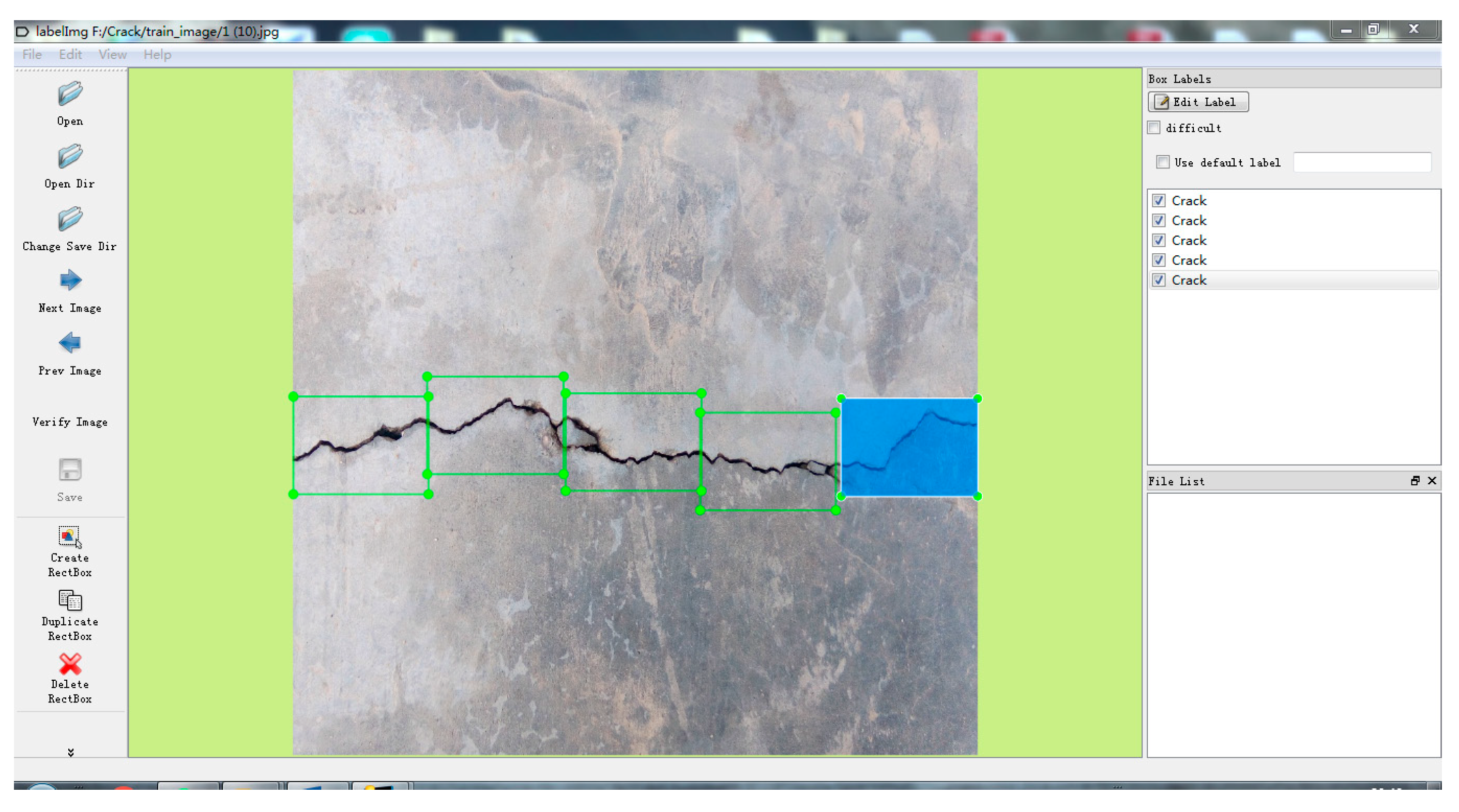
2.3. Crack Detection Dataset Build

In the course of the experiment, the dataset played an important role; 1600 of the original pictures were used as the training set, and 200 original pictures were used as the test set. The LabelImg tool was used to mark the crack location and category of the image, generate an XML file, and then, convert it to a TXT file, which contains the category of the crack, the centre coordinates, and the length and width of the smallest bounding rectangle. The image labelling sample is shown in Figure 2.

Considering the speed of model training and the use of computer memory and video memory, all images are compressed to 416 × 416 pixels under the premise of ensuring the original image ratio, and the blank parts are filled with grey (128, 128, 128). To improve the generalization ability of the model, it is also necessary to perform data augmentation of the crack pictures, and the augmentation measures are the same as those of the crack recognition dataset.

3. Crack Recognition Based on Convolutional Neural Network

3.1. Model Building

In this research, we chose three classic neural networks, AlexNet, VGGNet16, and ResNet18, to conduct model training. First, we use the training dataset to train these three kinds of neural networks, input the training dataset into the neural network, and optimize according to the loss function. After a certain epoch, the neural network tends to converge and, then, uses the validation dataset to select the best model and, finally, compares the superiority of the training model according to the test set; the most suitable model was selected based on the comparison of the experimental results. Compared with the traditional method, the method in this paper has better generalization and robustness, but the method in this paper requires a large dataset, and the model training time is longer.

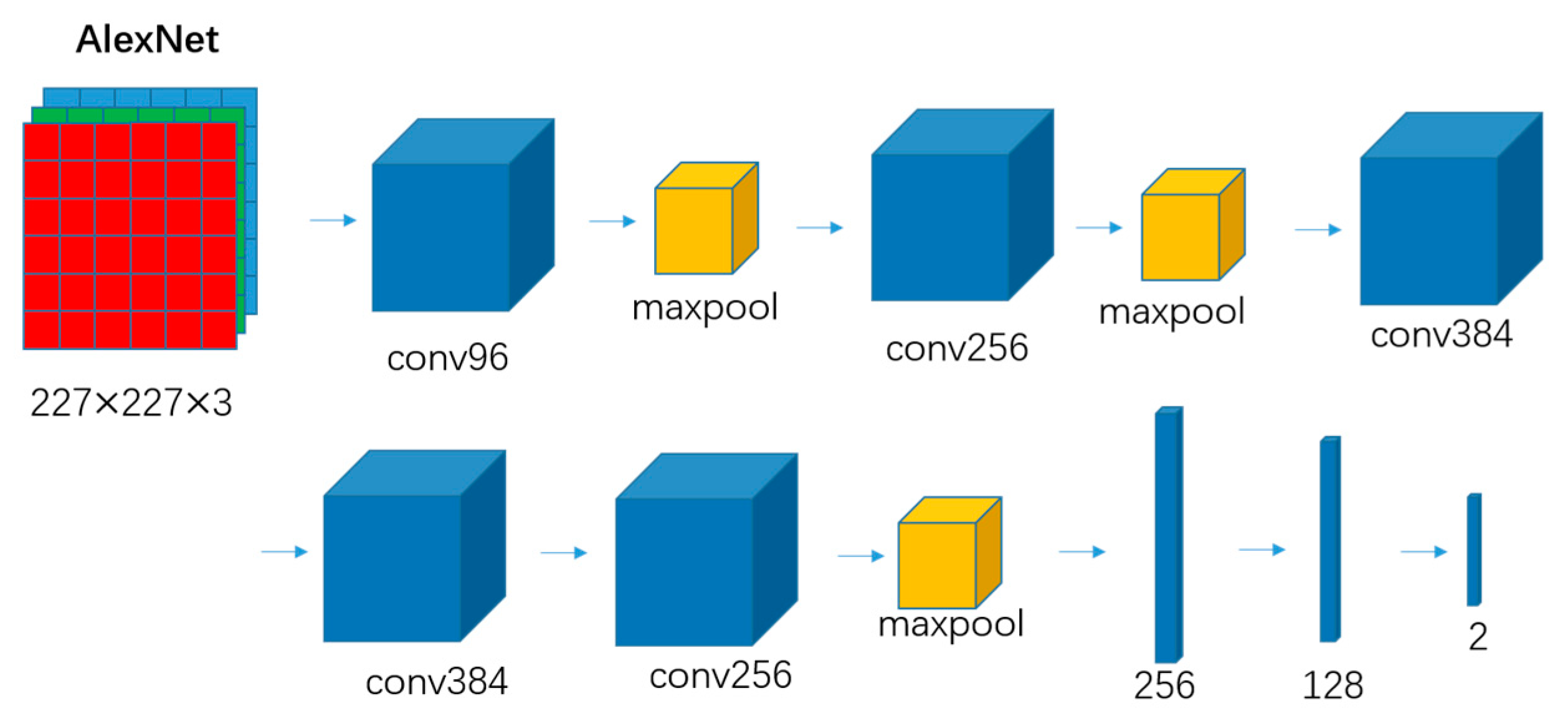
3.1.1. AlexNet Model

Figure 3 is the network structure of AlexNet. The model is divided into eight layers, including five convolutional layers and three fully connected layers. The input is an image of 227 × 227 × 3 pixels, the blue square is the convolutional layer, the yellow square is the pooling layer, and the blue strip is the fully connected layer. The size of the convolutional layer is 5 × 5 × 96, 3 × 3 × 256, 3 × 3 × 384, 3 × 3 × 256, and 3 × 3 × 256, the size of the pooling layer is 3×3, and the number of neurons in the fully connected layer is 256, 128, and 2, respectively.

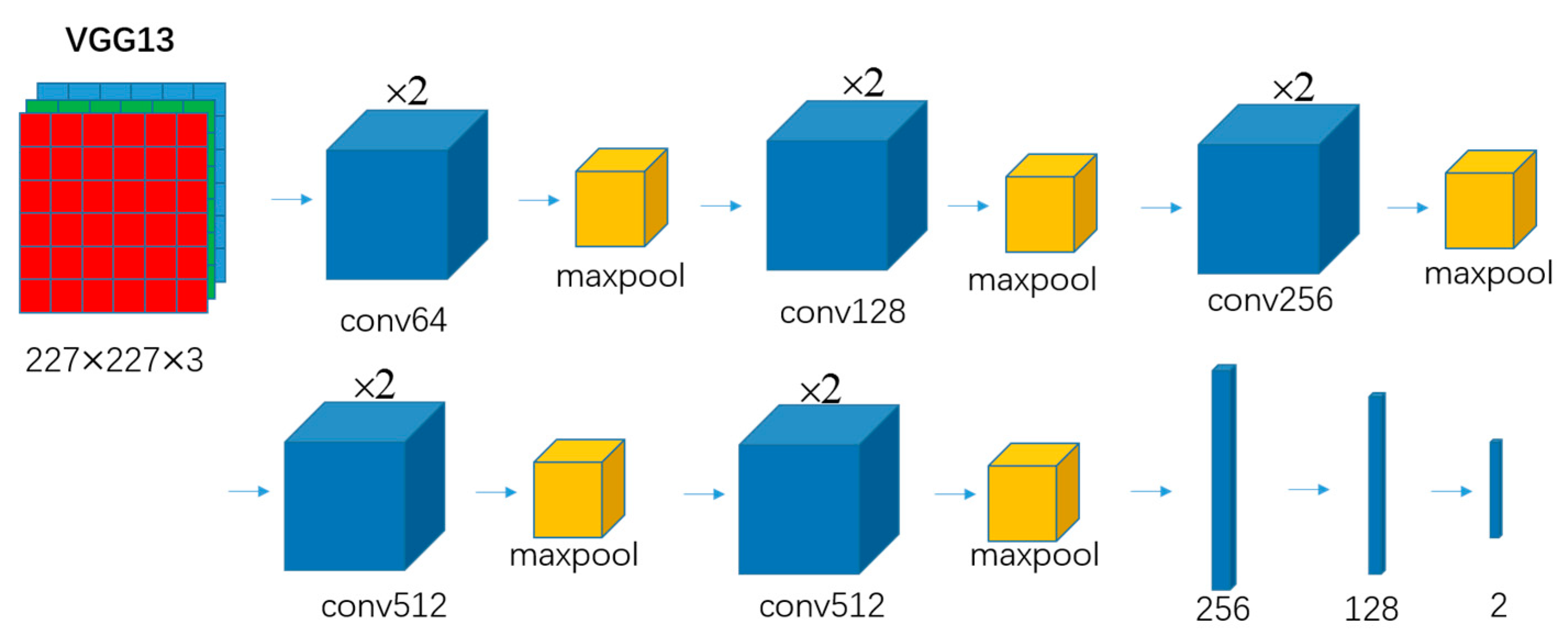
3.1.2. VGGNet13 Model

Figure 4 is the network structure of VGGNet13. The model is divided into 13 layers, including 10 convolutional layers and three fully connected layers. The number ×2 represents two convolutions of the same size, a total of 10 convolutional layers, there are four types of convolutional layers, whose sizes are 3 × 3 × 64, 3 × 3 × 128, 3 × 3 × 256, 3 × 3 × 512.

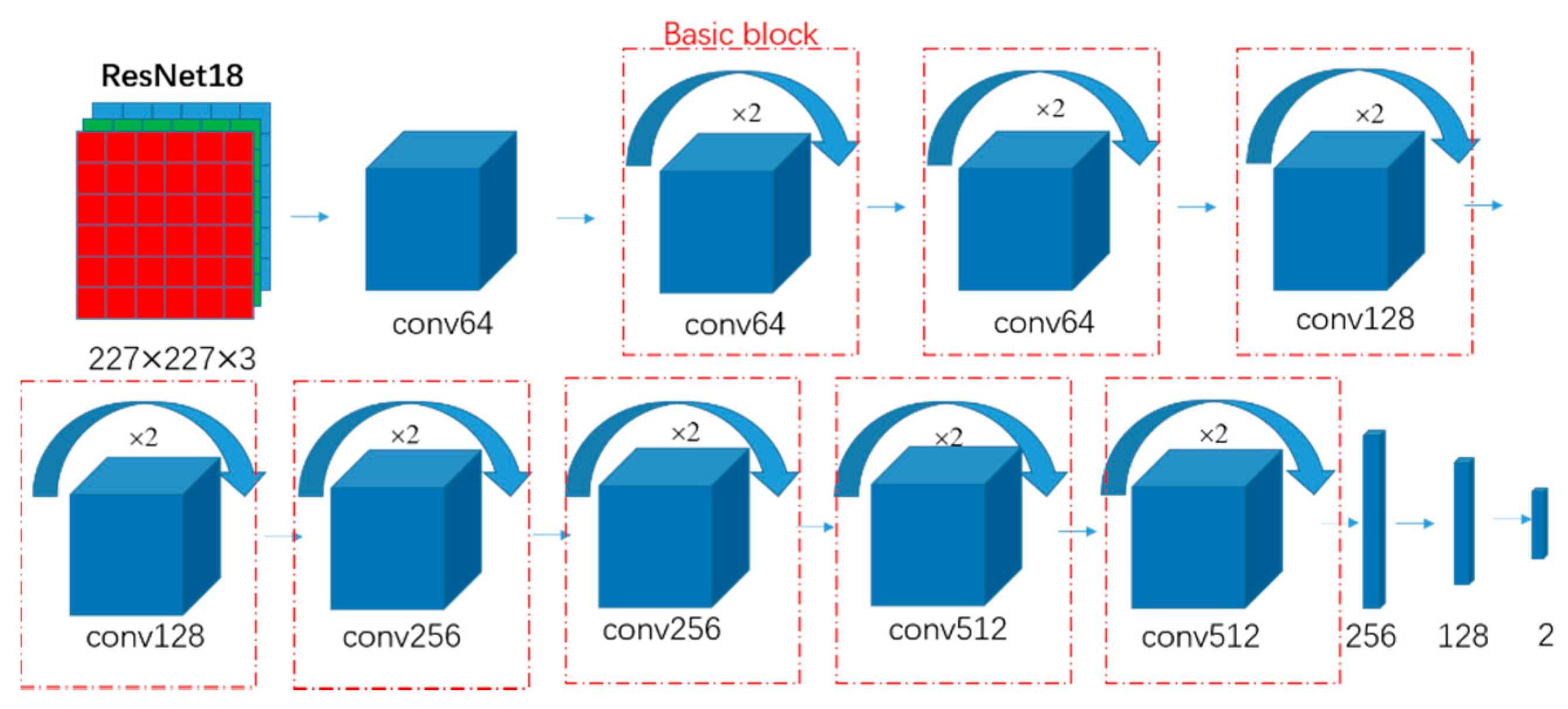
3.1.3. ResNet18 Model

Figure 5 is the network structure of ResNetNet18. There are 8 basic block modules in the red dotted area, and each module’s blue arrow is a short connection. This means that the neural network can be deeper because the gradient can transfer farther during backpropagation. The model is divided into 20 layers, including 17 convolutional layers and three fully connected layers. The pooling layer is not shown in the figure but exists after each convolutional layer. The specific parameters of the ResNet18 model are the same as those of the VGGNet13 model.

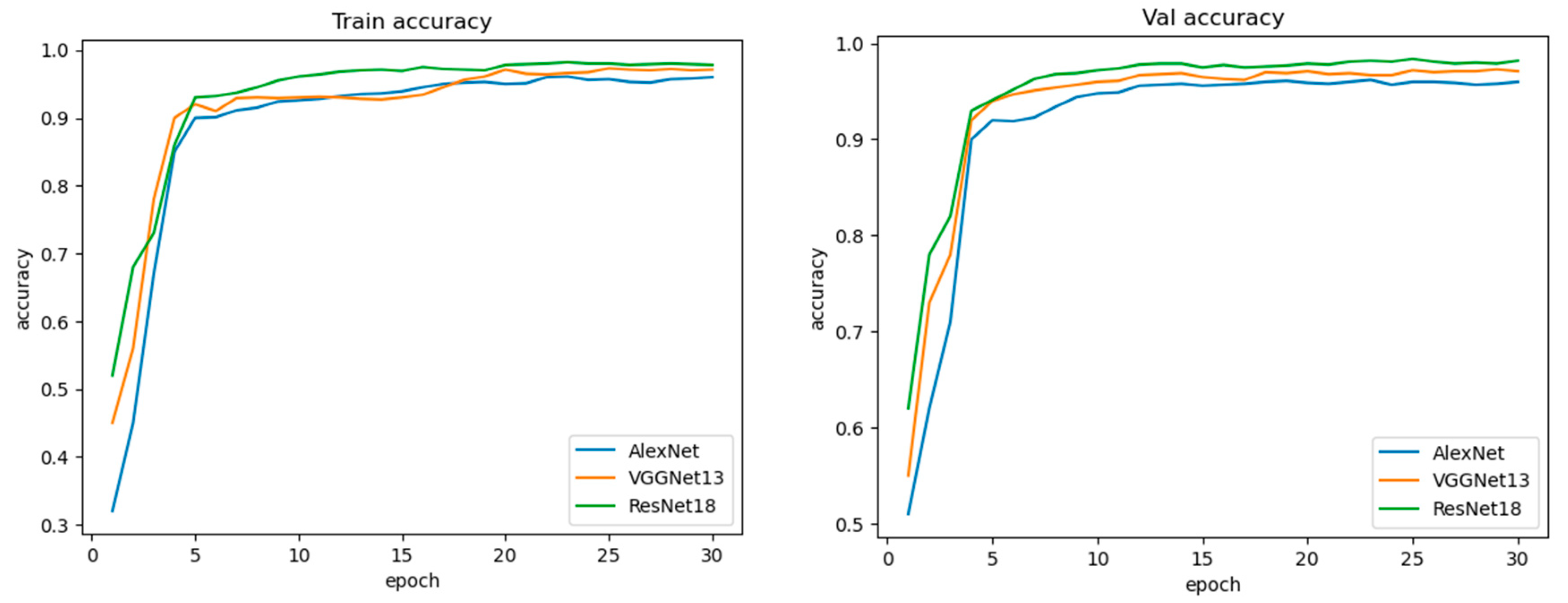
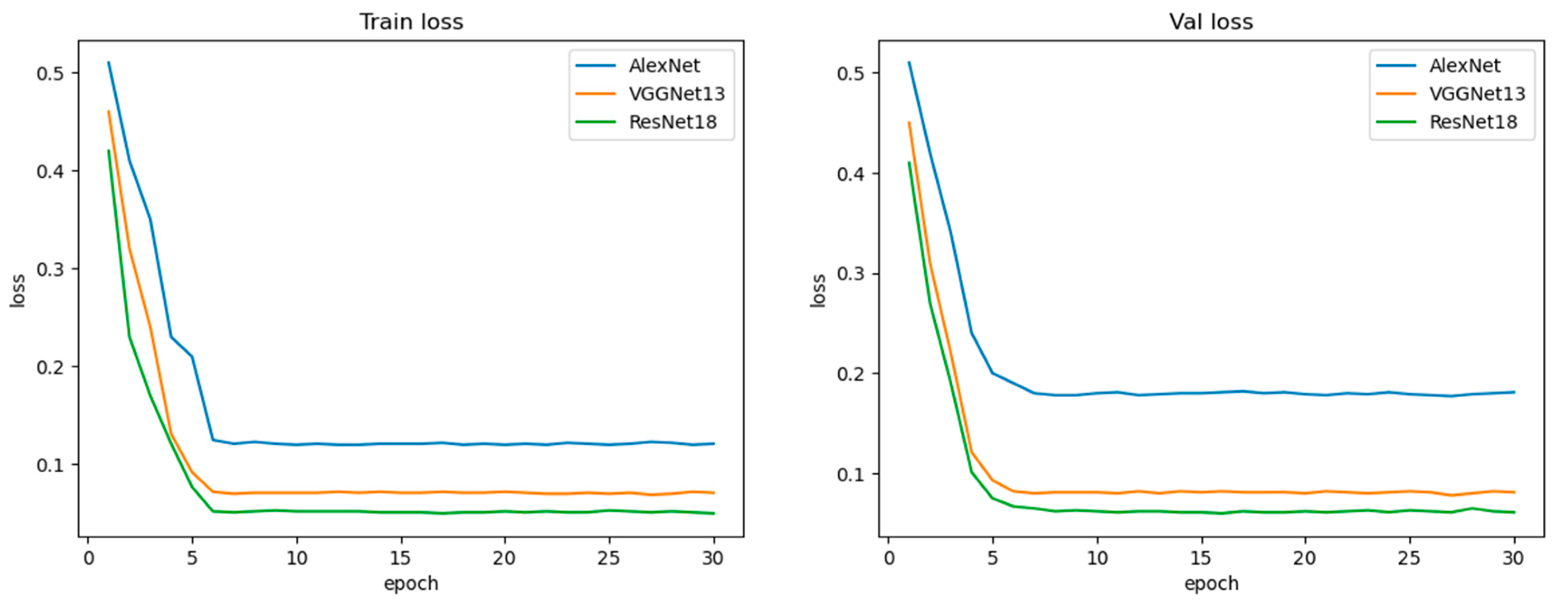
3.2. Experimental Results and Analysis

In this experiment, 10,000 crack and 10,000 non-crack pictures were randomly shuffled, and 3000 pictures were selected as the validation set, which was used to select the best model; 3000 pictures were selected as the test set, and the test set was used to test the performance of the model; 14,000 pictures were the training set, which was used to train the model. To prevent over-fitting, measures such as batch normalization, regularization, and dropout were used. Normalization normalizes the pixel value of the input image to (0,1), which is easy for neural network convergence. Regularization adds a regular term to the loss function, and the value of the loss function becomes the sum of the loss function and the regular term. Dropout indicates that a random part of the neuron parameters is not updated every time it is back propagated. The platform of this experiment is based on the Ubuntu platform, the programming language is Python, and the frameworks are TensorFlow, Keras, and OpenCV. The initial learning rate is 0.001, and epoch is 30.

Figure 6 shows the accuracy curve of the training and validation dataset. Our curve shows that ResNet18 has a better performance than other neural networks in training and validation accuracy.

Figure 7 shows the loss function curve of the training and validation dataset. The curve also revealed a significant difference between the loss, and ResNet18 had a lower loss than AlexNet and VGGNet13.

3.3. Evaluation Index

The experiment uses a confusion matrix to evaluate the network model, which is shown in

Table 1. Confusion matrix.

Real	Predict
	I	II
I	TP( True Positive)	FN (False Negative)
II	FP (False Positive)	TN (True Negative)

. The total number of samples in each column is the predicted category, the total number of samples in each row is the actual category, and the total number of samples on the diagonal is the correct samples classified by the model.

According to the test dataset, the ratio of the correct value predicted by the model to the total value is defined as the accuracy rate, as shown in Equation (1):

$$Acc=\frac{\mathrm{TP}+\mathrm{TN}}{\mathrm{TP}+\mathrm{FP}+\mathrm{FN}+\mathrm{TN}}$$

(1)

Accuracy is the most common evaluation indicator, but for a certain case, it is difficult to derive the accuracy rate. Thus, a so-called “precision rate” can be used instead. The precision rate is defined as follows:

$$P=\frac{\mathrm{TP}}{\mathrm{TP}+\mathrm{FP}}$$

(2)

In addition, the so-called “recall rate” and “$F_1$ score” were used to evaluate the network model. The recall rate is the proportion of all real I (TP + FN) that are judged to be class I (TP), as shown in Equation (3):

$$R=\frac{\mathrm{TP}}{\mathrm{TP}+\mathrm{FN}}$$

(3)

The relationship between the $F_1$ score and the precision rate as well as the recall rate is shown in Equation (4):

$$\frac{2}{F_1}=\frac{1}{P}+\frac{1}{R}$$

(4)

From the above analysis and

Table 2. Experimental results.

Categories	Acc	P	R	${\mathit{F}}_1$
AlexNet	97.6%	97.9%	97.3%	97.6%
VGG13	98.3%	98.6%	98%	98.3%
ResNet18	98.8%	98.9%	98.6%	98.8%

, under the premise of training 30 epochs at the same time, the ResNet18 model’s accuracy, precision, recall, and F1 in the test set are better than those of the other two neural networks. It shows that the ResNet18 model has better performance than other models in the crack dataset, so we take the ResNet18 model as our final recognition model.

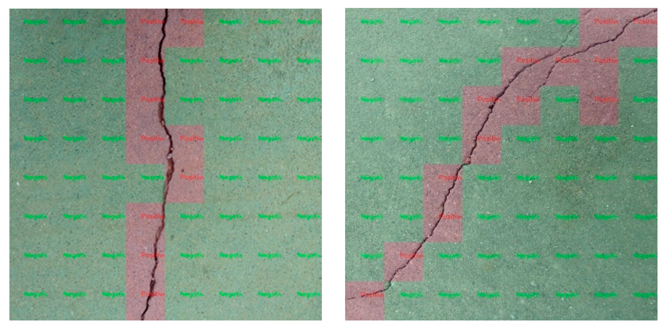
3.4. Real Image Test

It is impossible for the actual picture to have a resolution of 227 × 227 pixels, which may be 1024 × 1024 pixels or even larger. Therefore, we generally use a sliding window method, and we choose a 227 × 227 pixel window to slide. When a small area is recognized as a crack, the image area is marked as red and marked as positive. When it is not a crack, the image area is marked as negative. Slide from left to right, top to bottom, and the result is shown in Figure 8.

4. Crack Detection Based on YOLOv3

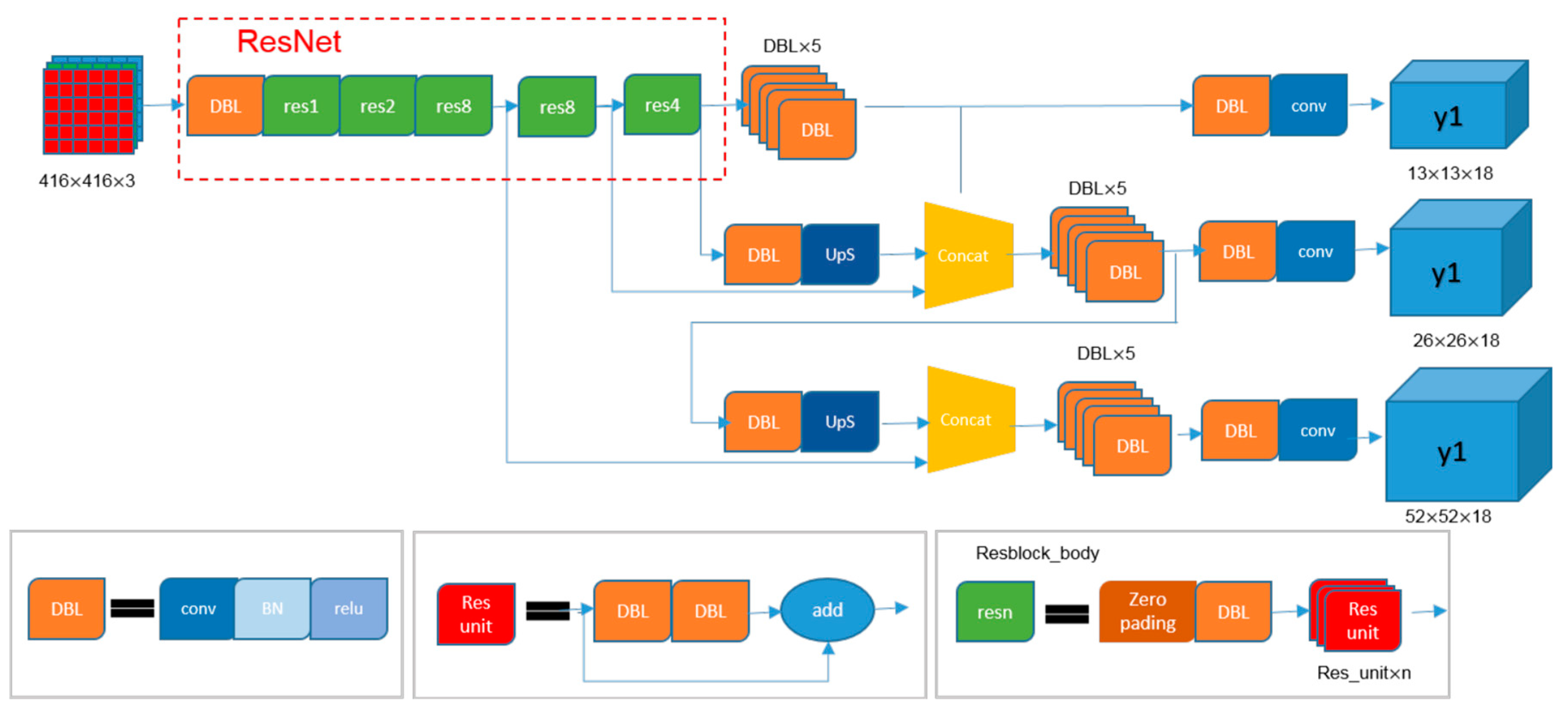
4.1. Model Building

In 2018, Redmon et al. [29] released a new algorithm, YOLOv3, which adopts some of today’s better target detection ideas, into YOLO. Under the premise of ensuring a speed advantage, the detection accuracy is further improved, especially the detection ability for small objects. YOLOv3 mainly improves the network structure. The network structure is introduced below.

The network structure of YOLOv3 is shown in Figure 9. The network input image size is 416 × 416 × 3. The meaning of each module in the figure is as follows:

• DBL represents the combination of convolution, BN and leaky ReLU. In YOLOv3, the convolutional layer appears as such components and constitutes the basic unit of DarkNet. The number after DBL indicates that there are several DBL modules.
• Res: Res in the figure represents the residual module, which is essentially a residual network. The number after Res represents several residual modules connected in series.
• Up-sampling: up-sampling uses up-pooling, that is, the method of element replication and expansion makes the feature size expand, and without learning parameters.
• Concat: after up-sampling, the deep and shallow feature maps are subjected to the Concat operation, that is, channel-wise splicing.

YOLOv3 algorithm process: First input an image, and go through multiple Res modules; the first module is the deep feature output, which produces a smaller feature map and can detect larger cracks. The second is the deep feature and the penultimate layer output feature Concat produces a medium-sized feature map and can detect medium-sized cracks. The third is the Concat of deep features and the third-to-last layer feature to produce a relatively large feature map, which can detect small cracks. The advantage of this is that it can detect multi-scale targets in the images and avoid the problem of missed detection.

We can also see some advantages in the DarkNet-53 network structure in Figure 9:

• Residual idea: DarkNet-53 draws on ResNet’s residual idea and uses a large number of residual connections in the basic network, so the network structure can be designed very deep, and the gradient can be transmitted farther and relieved when the gradient is back propagated. The problem of gradient disappearance during training is solved, which makes the model easier to converge.
• Multi-layer feature maps: Through up-sampling and Concat operations, deep and shallow features are merged, and finally, feature maps of three sizes are output for subsequent prediction. Multi-layer feature maps have obvious advantages when detecting multi-scale objects or small objects.
• Without the pooling layer: The previous YOLO network has five maximum pooling layers to reduce the size of the feature map, but YOLO v3 down sampling achieves the same effect of reducing the size. The number of down-sampling is also five, and the overall sampling frequency is 32.

4.2. Loss Function

YOLOv3 uses the mean square and error as the loss function. It consists of three parts: coordinate error, IOU error, and classification error.

$$Loss={\displaystyle \sum }_{i=0}^{s^2}coordErr+iouErr+clsErr$$

(5)

In simple addition, the contribution rate of each loss should be considered. YOLOv3 sets the weight ${\lambda }_{coord}=5$ for coordErr. When calculating the IOU error, the grid containing the object, and the grid without the object, the IOU error of the two contributes to the network loss, and the values are different. If the same weight is used, the confidence value of the grid that does not contain the object is approximately 0, which in disguise amplifies the influence of the confidence error of the grid that contains the object in calculating the gradient of the network parameters. To solve this problem, YOLOv3 uses ${\lambda }_{noobj}=0.5$ to correct iouErr. For equal error values, the impact of large object errors on detection should be less than the impact of small object errors on detection. This is because the proportion of the same position deviation in large objects is much smaller than the proportion of the same deviation in small objects. YOLOv3 takes the square root of the object size information items (w and h) to improve this problem, but it cannot completely solve this problem.

In summary, the loss calculation of YOLOv3 during training is as follows:

$$\begin{array}{cc}Loss=& {\lambda }_{coord}{\displaystyle {\displaystyle \sum }_{i=0}^{s^2}}{\displaystyle {\displaystyle \sum }_{j=0}^B}{I}_{ij}^{obj}\left[{\left(x_i-{\widehat{x}}_i\right)}^2+{(y_i-{\widehat{y}}_i)}^2\right]+{\lambda }_{coord}{\displaystyle {\displaystyle \sum }_{i=0}^{s^2}}{\displaystyle {\displaystyle \sum }_{j=0}^B}{I}_{ij}^{obj}\left[{\left(\sqrt{w_i}-\sqrt{{\widehat{w}}_i}\right)}^2+{\left(\sqrt{h_i}-\sqrt{{\widehat{h}}_i}\right)}^2\right]\\ & +{\displaystyle {\displaystyle \sum }_{i=0}^{s^2}{\displaystyle \sum }_{j=0}^B}{I}_{ij}^{obj}{\left(C_i-{\widehat{C}}_i\right)}^2+{\lambda }_{noobj}{\displaystyle {\displaystyle \sum }_{i=0}^{s^2}{\displaystyle \sum }_{j=0}^B}{I}_{ij}^{noobj}{\left(C_i-{\widehat{C}}_i\right)}^2+{\displaystyle {\displaystyle \sum }_{i=0}^{s^2}}{I}_i^{obj}{\displaystyle {\displaystyle \sum }_{c\in classes}}{\left(p_i\left(c\right)-{\widehat{p}}_i\left(c\right)\right)}^2\end{array}$$

(6)

$\left(x,y,w,h,C,p\right)$ is the true value, and $\left(\widehat{x},\widehat{y},\widehat{w},\widehat{h},\widehat{C},\widehat{p}\right)$ is the predicted value. $I_{ij}^{obj}$ indicates that the object falls into box j of grid i. If there is no target in the box, the classification error is not back propagated. The loss function is used to back propagate and update the parameters of YOLOv3 until convergence.

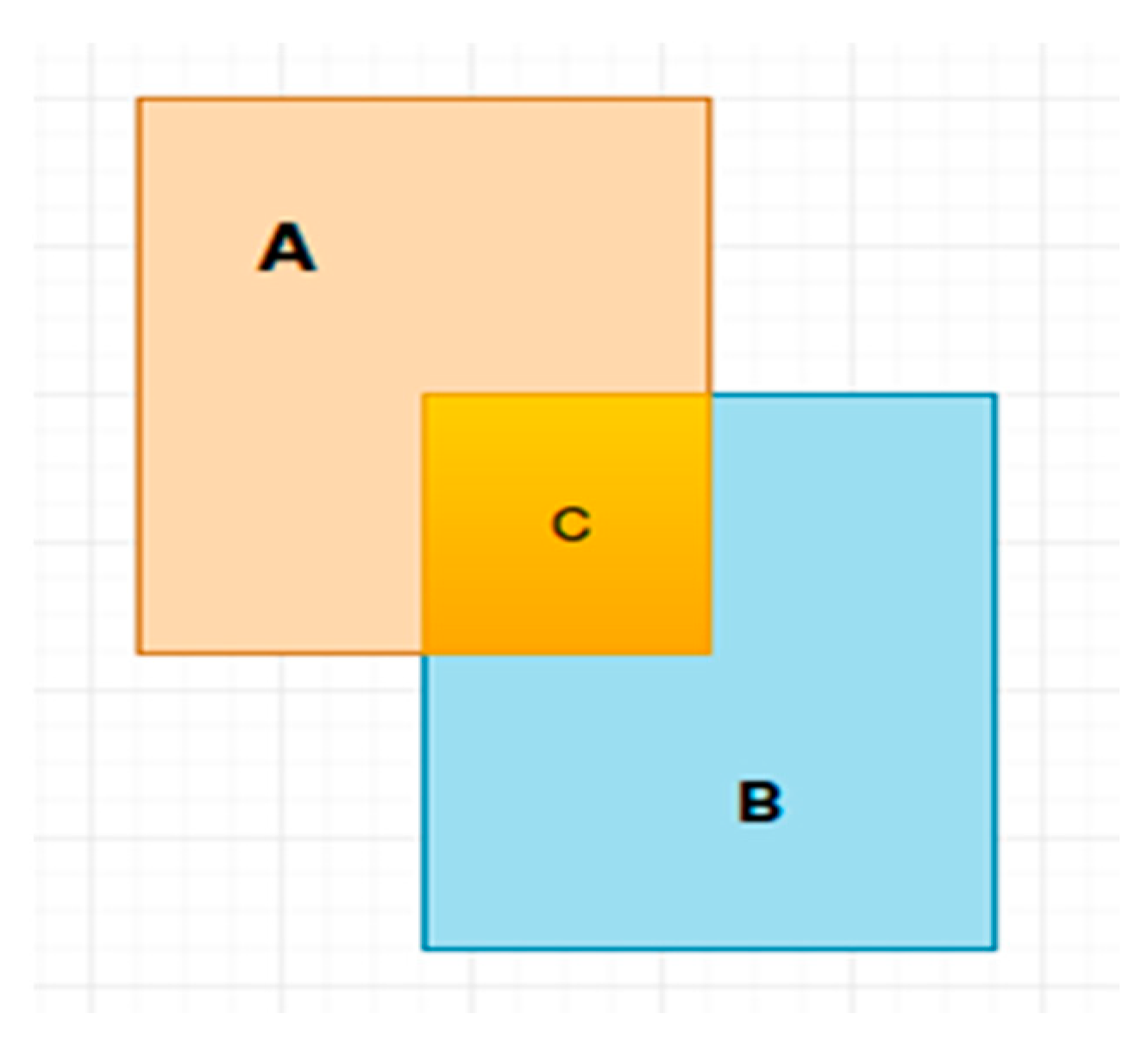
4.3. Evaluation Index

Intersection over union (IOU) is a standard for measuring the accuracy of detecting objects. It refers to the ratio of the intersection and union between the suggested box and the real box predicted by the model. As shown in Figure 10, A is the suggested box, B is the real box, the union of set A and set B includes all parts of A and B, and set C is the intersection of set A and set B. If A and B completely overlap, it means that the value of IOU is 1, and the model performances are perfect. If A and B do not overlap, it means that the value of IOU is 0, and the model performances are poor.

$$\mathrm{IOU}=\frac{\mathrm{A}\cap \mathrm{B}}{\mathrm{A}\cup \mathrm{B}}$$

(7)

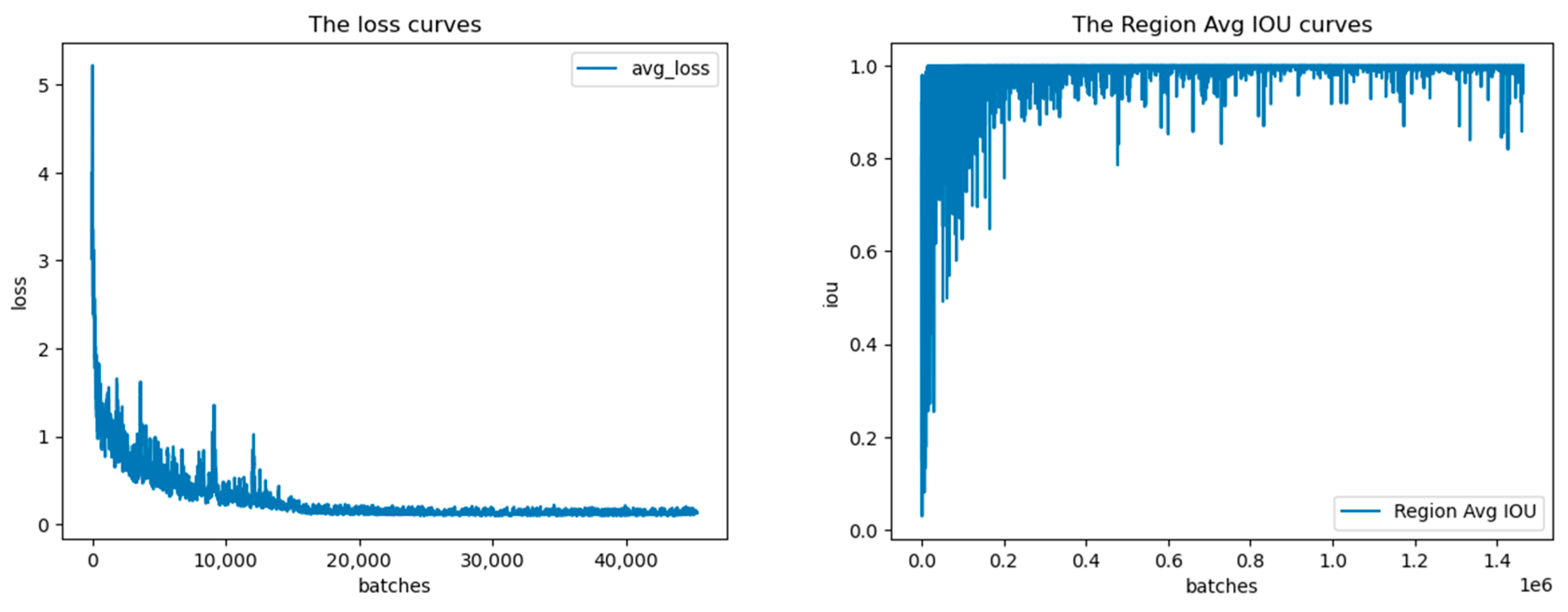
4.4. Experimental Results and Analysis

This experiment relies on transfer learning and initializes Darknet-53 parameters, which were trained on the ImageNet dataset. The batch size is 16, the maximum number of training batches is 50,020, the activation function is the leaky ReLU, and the optimizer uses the stochastic gradient descent algorithm (stochastic gradient descent, SGD [30]). The initial learning rate is 0.001, momentum is 0.9, and the weight decay coefficient is 0.0005. When iterating to 30,000 times, the learning rate is changed to 0.0001, and when iterating to 40,000 times, the learning rate is changed to 0.00001, iterate to 50,020 times or stop training when the loss converges.

The left side of Figure 11 is the loss curve of YOLOv3, the abscissa is the number of training batches, and the ordinate is the loss value. The figure shows that the model is trained for 50,020 batches, and the loss fluctuates obviously before 15,000 batches; after 15,000 batches, the loss curve tends to converge. After 30,000 batches, the learning rate becomes one-tenth of the original, and the loss slightly decreases. After 40,000 batches, the learning rate changes one-tenth of the previous value, the loss curve converges, and the final loss converges to approximately 0.12. From the loss curve, the training performance of the model is good, and there is no over-fitting.

The right side of Figure 11 is the IOU curve of YOLOv3. The abscissa is the number of training batches, and the ordinate is the IOU value. Because each batch has a different IOU value, the maximum value of the abscissa is not 50,020. As seen in the figure, the value of IOU fluctuates greatly before 15,000 batches. After that, it tends to converge, the value focusing on approximately 0.9, and the model’s result shows that the suggested box and real label box overlap.

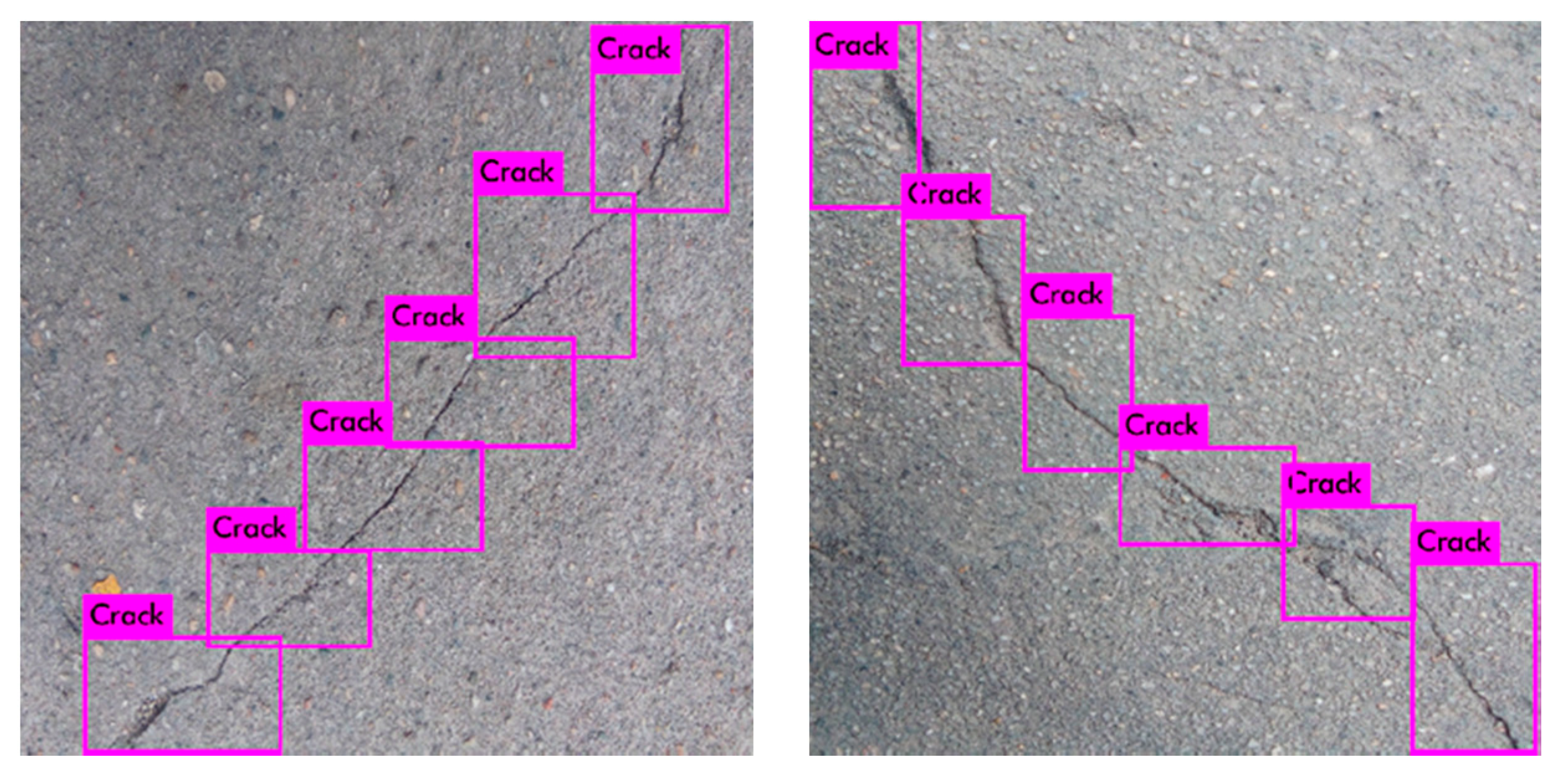
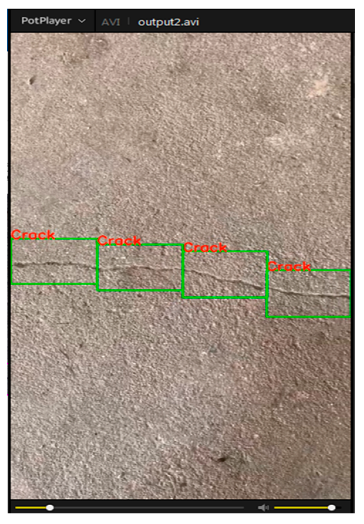
4.5. Real Image and Video Test

Using the trained model to detect the crack pictures in the test set, some of the results of the test set detection are shown in Figure 12. It can be seen in the figure that this method can effectively detect cracks and perform classification.

A short video of the crack was collected with a mobile phone and sent to the trained model for crack detection. The video was collected with an iPhone7 camera, the time of the video was 13 s, and the resolution was 544 × 960 pixels. The test results are shown in Figure 13. The trained model can better detect the crack area in the video. Even if the image size of the input model was different from the training set, the crack was still accurately detected, indicating that the overall generalization performance of the model is very good.

5. Conclusions

Three kinds of neural networks are used to recognize crack images. In this experiment, we can see that ResNet18 is better than the other two neural networks. In the real world, the types of crack images will be very rich. How to better extract features from images and accurately recognize cracks is difficult. We can see from the structure of the model that the structure of AlexNet is relatively simple, and there are few convolutional layers, the depth of the model is relatively shallow, while the convolutional layer of VGGNet13 is more, and the depth of the model is also deeper, and its performance is better than AlexNet. It can be seen that the deepening of the neural network can better extract the features in images, but when the model is blindly deepened, the performance may not always be good because the gradient vanishes during optimization, which causes the neural network to fail to converge. Therefore, ResNet18 solves the vanishing gradient problem. It can be seen in the model diagram that it is a short connection so that during optimization, the gradient is propagated back and there is no gradient vanish, which makes the neural network easy to converge. Therefore, in practical applications, ResNet18 has a deeper depth and short connection, so the features in the image can be better extracted and cracks can be recognized.

In the second part of the study, we mainly trained the YOLOv3 model for crack target detection on crack images. We can clearly see from the loss curve that the model finally converged, but in the IOU curve, we can see that it oscillates afterwards; that is, the prediction box and the real box never overlap perfectly. The reason may be that when the training dataset is built, there will be a small amount of overlap between the labelled box when the crack image is labelled (refer to Figure 2). However, in the actual video and picture test, the model performance is still good, and the crack area in the picture and video can be accurately detected. The disadvantage is that the detection box has a small overlap, which is also part of later research.

In practice, the method in this article can be extended to real-world structures to realize more effective and reliable monitoring. For example, drones are used to carry cameras to quickly take videos and images related to roads and bridges (concrete structures), wireless transmission is used to the local end, and then, the method in this article is used to input the images and videos into the model. ResNet18 can quickly recognize cracked images and then use the YOLOv3 model to detect the crack area of the crack images and video. The trained model can accurately detect and recognize the crack area. In addition, thanks to the advantages of YOLOv3 in target detection speed, the method proposed in this paper can meet the requirements of crack detection speed. There are broad application prospects in the real-time detection of cracks.

References

1. Albishi, A.M.; Ramahi, O.M. Surface crack detection in metallic materials using sensitive microwave-based sensors. In Proceedings of the 2016 IEEE Annual Wireless and Microwave Technology Conference, Clearwater, FL, USA, 11–13 April 2016. [Google Scholar]
2. Lacidogna, G.; Piana, G.; Accornero, F.; Carpinteri, A. Multi-technique damage monitoring of concrete beams: Acoustic Emission, Digital Image Correlation, Dynamic Identification. Constr. Build. Mater. 2020, 242, 118114. [Google Scholar] [CrossRef]
3. Liu, P.; Lim, H.; Yang, S.; Sohn, H. Development of a “stick-and-detect” wireless sensor node for fatigue crack detection. Struct. Health Monit. 2016, 16, 153–163. [Google Scholar] [CrossRef]
4. Zhao, S.; Sun, L.; Gao, J.; Wang, J. Uniaxial ACFM detection system for metal crack size estimation using magnetic signature waveform analysis. Measurement 2020, 164, 108090. [Google Scholar] [CrossRef]
5. Yang, X.; Zhou, Z. Design of crack detection system. In Proceedings of the 2017 International Conference on Network and Information Systems for Computers, Shanghai, China, 14–16 April 2017. [Google Scholar]
6. Zhang, X.; Wang, K.; Wang, Y.; Shen, Y.; Hu, H. Rail crack detection using acoustic emission technique by joint optimization noise clustering and time window feature detection. Appl. Acoust. 2020, 160, 107141. [Google Scholar] [CrossRef]
7. Amhaz, R.; Chambon, S.; Jerome, I. Automatic Crack Detection on Two-Dimensional Pavement Images: An Algorithm Based on Minimal Path Selection. Trans. Intell. Transp. Syst. 2016, 17, 2718–2729. [Google Scholar] [CrossRef] [Green Version]
8. Amhaz, R.; Chambon, S.; Jerome, I.; Baltazart, V. A new minimal path selection algorithm for automatic crack detection on pavement images. In Proceedings of the 2014 International Conference on Image Processing, Paris, France, 27–30 January 2014. [Google Scholar]
9. Yang, L.C.; Vincent, B.; Rabih, A.; Peilin, J. A new A-star algorithm adapted to the semi-automatic detection of cracks within grey level pavement images. In Proceedings of the 2016 International Conference on Digital Image Processing, Chengdu, China, 20–22 May 2016. [Google Scholar]
10. Cheon, M.H.; Hong, D.G.; Lee, D.H. Surface crack detection in concrete structures using image processing. In Proceedings of the 2017 International Conference on Robot Intelligence Technology and Applications, Daejeon, Korea, 14–15 December 2017. [Google Scholar]
11. Tedeschi, A.; Benedetto, F. A real-time automatic pavement crack and pothole recognition system for mobile Android-based devices. Adv. Eng. Inform. 2017, 32, 11–25. [Google Scholar] [CrossRef]
12. Xiao, Y.; Zhang, H. Research on Surface Crack Detection Technology Based on Digital Image Processing. In Proceedings of the 2019 International Workshop on Advanced Algorithms and Control Engineering, Shenzhen, China, 21–22 February 2020. [Google Scholar]
13. Sun, H.; Liu, Q.; Fang, L. Research on Fatigue Crack Growth Detection of M(T) Specimen Based on Image Processing Technology. J. Fail. Anal. Prev. 2018, 18, 1010–1016. [Google Scholar] [CrossRef]
14. Wang, Y.; Huang, Y.; Huang, W. Crack junction detection in pavement image using correlation structure analysis and iterative tensor voting. IEEE Access 2019, 7, 138094–138109. [Google Scholar] [CrossRef]
15. Li, W.; Ju, H.; Susan, L.; Ren, Q. Three-dimensional pavement crack detection algorithm based on two-dimensional empirical mode decomposition. J. Transp. Eng. Part B Pavements 2017, 143, 2573–5438. [Google Scholar] [CrossRef]
16. Wang, S.; Yang, F.; Cheng, Y.; Yang, Y.; Wang, Y. Adaboost-based Crack Detection Method for Pavement. In Proceedings of the 2018 International Conference on Civil and Hydraulic Engineering, Qingdao, China, 23–25 November 2018. [Google Scholar]
17. Freund, Y.; Schapire, R. A Decision-Theoretic Generalization of On-Line Learning and an Application to Boosting. J. Comput. Syst. Sci. 1996, 55, 119–139. [Google Scholar] [CrossRef] [Green Version]
18. Sharma, S.; Gupta, N.K. A Genetic Approach to Segment and Detect Crack in Rail Track. In Proceedings of the 2019 International Conference on Computing Methodologies and Communication, Erode, India, 27–29 March 2019. [Google Scholar]
19. Yusof, N.; Osman, M.; Hussain, Z.; Noor, M. Automated Asphalt Pavement Crack Detection and Classification using Deep Convolution Neural Network. In Proceedings of the 2019 International Conference on Control System, Penang, Malaysia, 29 November–1 December 2019. [Google Scholar]
20. Gaith, M.; Sedaghat, A.; Assad, H.; Hiyasat, M. Neural Network usage in structural crack detection. In Proceedings of the 2015 International Conference on Industrial Engineering and Operations Management, Dubai, United Arab Emirates, 3–5 March 2015. [Google Scholar]
21. Liu, Z.; Cao, Y.; Wang, Y.; Wang, W. Computer vision-based concrete crack detection using U-net fully convolutional networks. Autom. Constr. 2019, 104, 129–139. [Google Scholar] [CrossRef]
22. Krizhevsky, A.; Sutskever, I.; Hinton, G. ImageNet classification with deep convolutional neural networks. In Proceedings of the 2012 International Conference on Advances in Neural Information Processing Systems, Lake Tahoe, NV, USA, 3–6 December 2012. [Google Scholar]
23. Simonyan, K.; Zisserman, A. Very deep convolutional networks for large-scale image recognition. In Proceedings of the 2015 International Conference on Learning Representations, San Diego, CA, USA, 7–9 May 2015. [Google Scholar]
24. He, K.; Zhang, X.; Ren, S.; Sun, J. Deep residual learning for image recognition. In Proceedings of the 2016 IEEE Computer Society Conference on Computer Vision and Pattern Recognition, Las Vegas, NV, USA, 27–30 June 2016. [Google Scholar]
25. Girshick, R. Fast R-CNN. In Proceedings of the 2015 IEEE International Conference on Computer Vision, Santiago, Chile, 7–13 December 2015. [Google Scholar]
26. Ren, S.; He, K.; Girshick, R. Faster R-CNN: Towards real-time object detection with region proposal networks. In Proceedings of the 2016 International Conference on Neural Information Processing Systems, Montreal, QC, Canada, 7–12 December 2015. [Google Scholar]
27. Liu, W.; Anguelov, D.; Erhan, D. SSD: Single shot multibox detector. In Proceedings of the 2016 European Conference on Computer Vision, Amsterdam, Netherlands, 11–14 October 2016. [Google Scholar]
28. Redmon, J.; Farhadi, A. YOLOv3: An Incremental Improvement. In Proceedings of the 2018 IEEE Conference on Computer Vision and Pattern Recognition, Salt Lake City, UT, USA, 19–21 June 2018. [Google Scholar]
29. Redmon, J.; Divvala, S.; Girshick, R. You only look once: Unified, real-time object detection. In Proceedings of the 2016 IEEE Conference on Computer Vision and Pattern Recognition, Las Vegas, NV, USA, 26 June–1 July 2016. [Google Scholar]
30. Bottou, L. Large-scale machine learning with stochastic gradient descent. In Proceedings of the 2010 Conference on Computational Statistics, Paris, France, 22–27 August 2010. [Google Scholar]
Figure 1. Image enhancement.
Applsci 11 02868 g001
Figure 2. Crack image mark.
Applsci 11 02868 g002
Figure 3. AlexNet model.
Applsci 11 02868 g003
Figure 4. VGGNet13 model.
Applsci 11 02868 g004
Figure 5. ResNet18 model.
Applsci 11 02868 g005
Figure 6. Accuracy curve.
Applsci 11 02868 g006
Figure 7. Loss curve.
Applsci 11 02868 g007
Figure 8. Image test.
Applsci 11 02868 g008
Figure 9. YOLOv3 model.
Applsci 11 02868 g009
Figure 10. Intersection and union ratio.
Applsci 11 02868 g010
Figure 11. Model training results.
Applsci 11 02868 g011
Figure 12. Image test.
Applsci 11 02868 g012
Figure 13. Video test.
Applsci 11 02868 g013