
Multiresolution Topology Optimization of Large-Deformation Path-Generation Compliant Mechanisms with Stress Constraints


Abstract
:1. Introduction
- Problem type I:
- The design of maximum-displacement mechanisms finds the topology for the largest displacement of predefined degrees of freedoms for a given load.
- Problem type II:
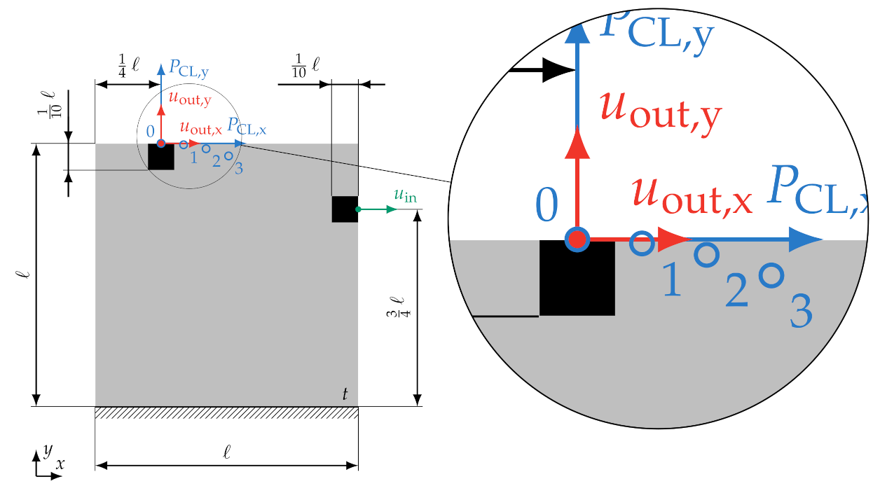
- The design of path-generation mechanisms finds the topology in which certain degrees of freedom are designed to go through predefined points (also known as way points or precision points), which describe a trajectory or path.
2. Topology Optimization for the Synthesis of Compliant Mechanisms
2.1. Nonlinear Finite-Element Analysis
2.2. Formulation of Topology Optimization
2.2.1. Design Variables and Their Stabilization
2.2.2. Maximum Displacement Objective Function
2.2.3. Path Generation Objective Function
2.2.4. Volume Constraint
2.2.5. Stress Constraint
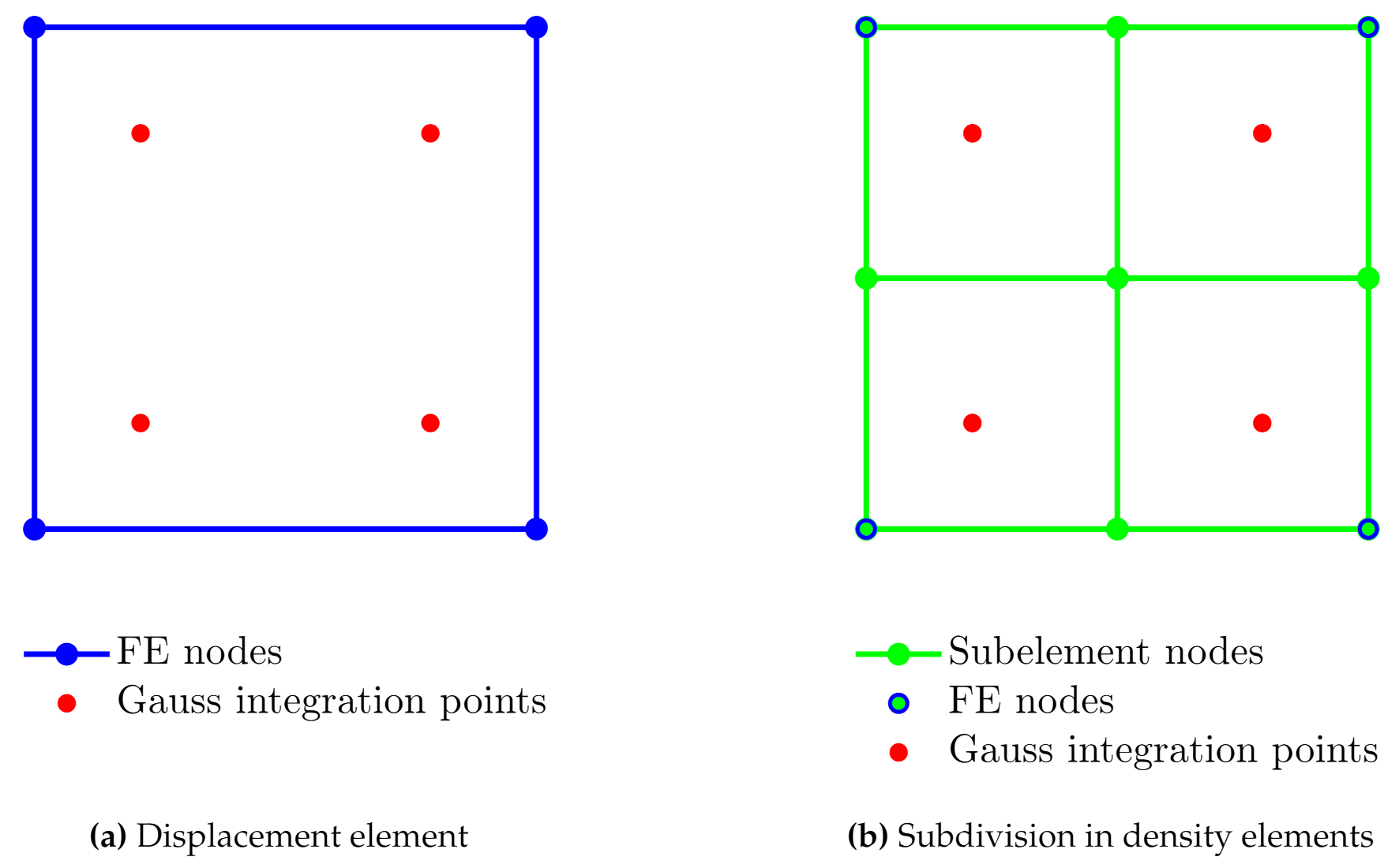
2.2.6. Multiresolution Topology Optimization
2.3. Design Sensitivity Analysis via Adjoint Methodology
2.3.1. Maximum Displacement Objective Sensitivity
2.3.2. Path Generation Objective Sensitivity
2.3.3. Volume Constraint Sensitivity
2.3.4. Stress Constraint Sensitivity
2.3.5. Sensitivity Analysis for Multiresolution Topology Optimization
3. Numerical Examples
3.1. Material and Constitutive Law
3.2. Numerical Example—Maximum Displacement Mechanism Design
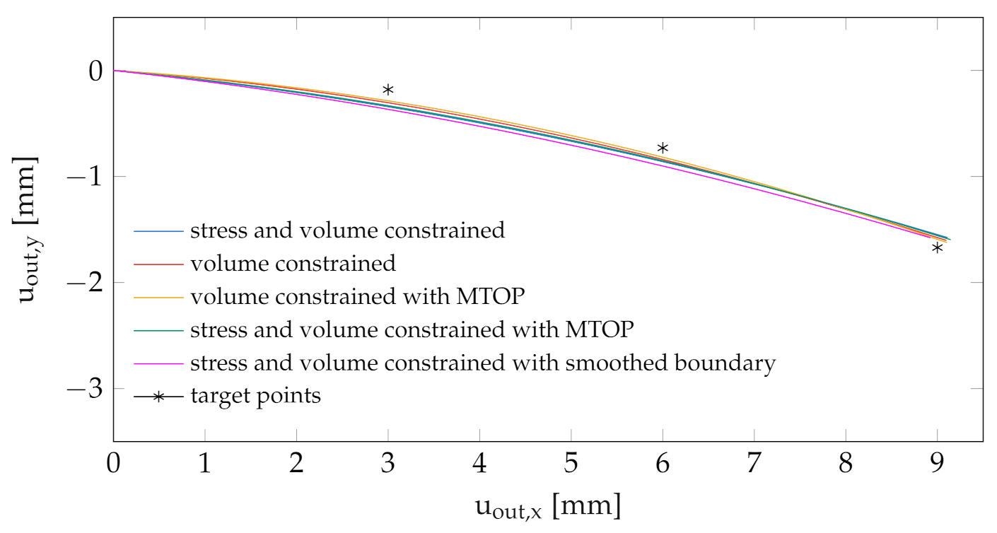
3.3. Numerical Example—Path-Generation Mechanism Design
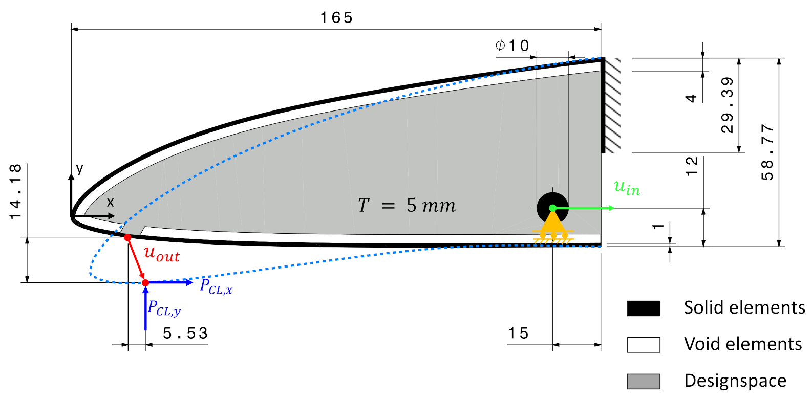
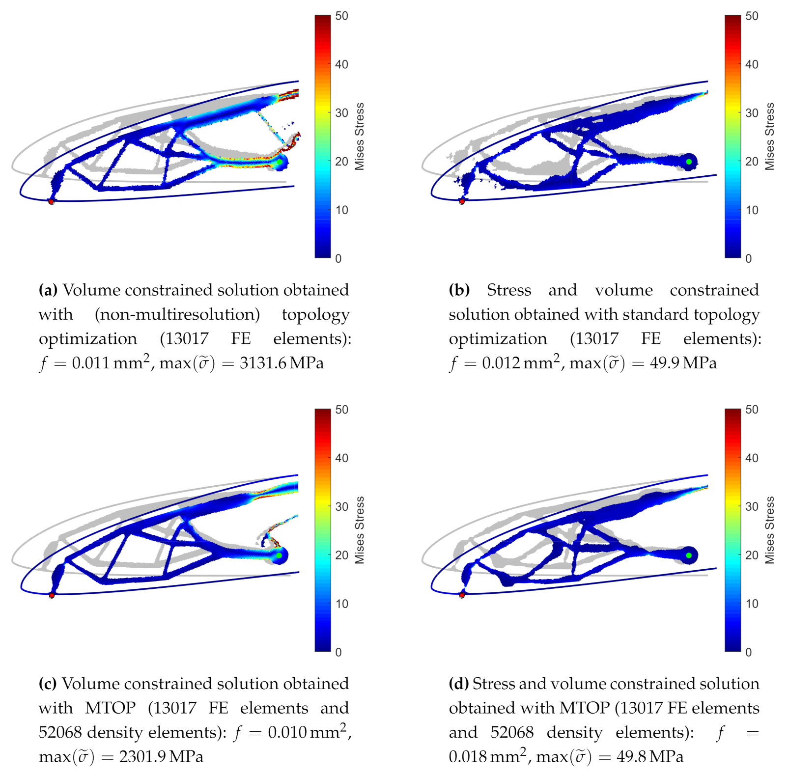
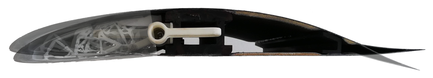
3.4. Engineering Example—Morphing Wing Design
4. Conclusions
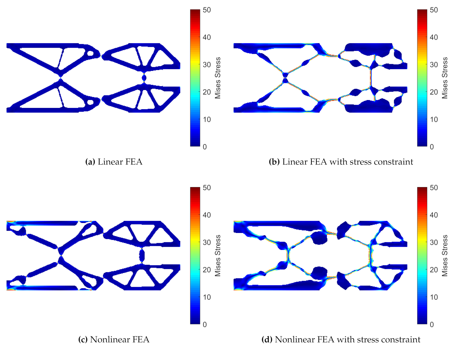
- linear finite-element analysis with volume constraint;
- linear finite-element analysis with volume and stress constraints;
- nonlinear finite-element analysis with volume constraint;
- nonlinear finite-element analysis with volume and stress constraints.
Author Contributions
Funding
Conflicts of Interest
References
- Howell, L. Compliant Mechanisms; A Wiley-Interscience Publication; Wiley: Hoboken, NJ, USA, 2001. [Google Scholar]
- Rojas, R.A.; Wehrle, E.; Vidoni, R. Optimal design for the passive control of vibration based limit cycles. Shock Vib. 2019, 2019, 1–11. [Google Scholar] [CrossRef]
- Michell, A. The limits of economy in frame-structures. Philos. Mag. 1904, 8, 589–597. [Google Scholar] [CrossRef] [Green Version]
- Bendsoe, M.P.; Kikuchi, N. Generating optimal topologies in structural design using a homogenization. Comput. Methods Appl. Mech. Eng. 1988, 71, 197–224. [Google Scholar] [CrossRef]
- Bendsoe, M.P. Optimal shape design as a material distribution problem. Struct. Optim. 1989, 1, 193–202. [Google Scholar] [CrossRef]
- Sigmund, O.; Petersson, J. Numerical instabilities in topology optimization: A survey on procedures dealing with checkerboards, mesh-dependencies and local minima. Struct. Multidiscip. Optim. 1998. [Google Scholar] [CrossRef]
- Sigmund, O. On the usefulness of non-gradient approaches in topology optimization. Struct. Multidiscip. Optim. 2011, 43, 589–596. [Google Scholar] [CrossRef]
- Baumgartner, A.; Harzheim, L.; Mattheck, C. SKO (soft kill option): The biological way to find an optimum structure topology. Int. J. Fatigue 1992, 14. [Google Scholar] [CrossRef]
- Tovar, A. Bone Remodeling as a Hybrid Cellular Automaton Process. Ph.D. Thesis, University of Notre Dame, South Bend, IN, USA, 2004. [Google Scholar]
- Svanberg, K. The method of moving asymptotes—A new method for structural optimization. Int. J. Numer. Methods Eng. 1987, 24, 359–373. [Google Scholar] [CrossRef]
- Ananthasuresh, G.; Kota, S.; Gianchandani, Y. A methodical approach to the design of compliant micromechanisms. Solid-State Sens. Actuator 1994, 189–192. [Google Scholar] [CrossRef]
- Sigmund, O. On the design of compliant mechanisms using topology optimization. Mech. Struct. Mach. 1997, 25, 493–524. [Google Scholar] [CrossRef]
- Zhu, B.; Zhang, X.; Zhang, H.; Liang, J.; Zang, H.; Li, H.; Wang, R. Design of compliant mechanisms using continuum topology optimization: A review. Mech. Mach. Theory 2020. [Google Scholar] [CrossRef]
- Pedersen, C.B.W.; Buhl, T.; Sigmund, O. Topology synthesis of large-displacement compliant mechanisms. Int. J. Numer. Methods Eng. 2001, 2683–2705. [Google Scholar] [CrossRef]
- Wehrle, E.J.; Han, Y.H.; Duddeck, F. Topology optimization of transient nonlinear structures—A comparative assessment of methods. In Proceedings of the 10th European LS-DYNA Conference, Würzburg, Germany, 15–17 June 2015. [Google Scholar]
- Park, G.J. Technical overview of the equivalent static loads method for non-linear static response structural optimization. Struct. Multidiscip. Optim. 2011, 43, 319–337. [Google Scholar] [CrossRef]
- Volz, K.H. Physikalisch begrndete Ersatzmodelle for die Crashoptimierung von Karosseriestrukturen in frhen Projektphasen. Ph.D. Thesis, Technische Universität München, Fachgebiet Computational Mechanics, Munich, Germany, 2011. [Google Scholar]
- Duddeck, F.; Volz, K. A new topology optimization approach for crashworthiness of passenger vehicles based on physically defined equivalent static loads. In Proceedings of the International Crashworthiness Conference, Milan, Italy, 18–20 July 2012. [Google Scholar]
- Duddeck, F.; Hunkeler, S.; Lozano, P.; Wehrle, E.; Zeng, D. Topology optimization for crashworthiness of thin-walled structures under axial impact using hybrid cellular automata. Struct. Multidiscip. Optim. 2016, 54, 415–428. [Google Scholar] [CrossRef]
- Dirksen, F.; Berg, T.; Lammering, R.; Zohdi, T.I. Topology synthesis of large-displacement compliant mechanisms with specific output motion paths. Proc. Appl. Math. Mech. 2012, 801–804. [Google Scholar] [CrossRef]
- Chen, Q.; Zhang, X.; Zhu, B. A 213-line topology optimization code for geometrically nonlinear. Struct. Multidiscip. Optim. 2019, 59, 1863–1879. [Google Scholar] [CrossRef]
- Stainko, R. An adaptive multilevel approach to the minimal compliance problem. Commun. Numer. Methods Eng. 2005, 22, 109–118. [Google Scholar] [CrossRef]
- de Sturler, E.; Paulino, G.; Wang, S. Topology Optimization with Adaptive Mesh Refinement. In Proceedings of the 6th International Conference on Computation of Shell and Spatial Structures, Ithaca, NY, USA, 28–31 May 2008. [Google Scholar]
- Borrvall, T.; Petersson, J. Large-scale topology optimization in 3D using parallel computing. Comput. Methods Appl. Mech. Eng. 2001, 190, 6201–6229. [Google Scholar] [CrossRef]
- Nguyen, T.H.; Paulino, G.H.; Song, J.; Le, C.H. A computational paradigm for multiresolution topology optimization (MTOP). Struct. Multidiscip. Optim. 2010, 41, 525–539. [Google Scholar] [CrossRef]
- Nguyen, T.H.; Paulino, G.; Song, J.; Le, C.H. Improving multiresolution topology optimization via multiple discretizations. Int. J. Numer. Methods Eng. 2012, 92, 507–530. [Google Scholar] [CrossRef]
- Duysinx, P.; Sigmund, O. New developments in handling stress constraints in optimal material distributions. In Proceedings of the 7th AIAA/USAF/NASA/ISSMO Symposium on Multidisciplinary Design Optimization, Saint Louis, MO, USA, 2–4 September 1998. [Google Scholar]
- De Leon, D.M.; Alexandersen, J.; Fonseca, J.S.O.; Sigmund, O. Stress-constrained topology optimization for compliant mechanism design. Struct. Multidiscip. Optim. 2015, 52, 929–943. [Google Scholar] [CrossRef] [Green Version]
- Conlan-Smith, C.; James, K.A. A stress-based topology optimization method for heterogeneous. Struct. Multidiscip. Optim. 2019, 60, 167–183. [Google Scholar] [CrossRef] [Green Version]
- De Leon, D.M.; Gonçalves, J.F.; de Souza, C.E. A Study on the Design of Large Displacement Compliant Mechanisms with a Strength Criteria Using Topology Optimization. In Advances in Structural and Multidisciplinary Optimization; Schumacher, A., Vietor, T., Fiebig, S., Bletzinger, K.U., Maute, K., Eds.; Springer International Publishing: Cham, Swizerland, 2018; pp. 952–966. [Google Scholar]
- Kreisselmeier, G.; Steinhauser, R. Systematic control design by optimizing a vector performance vector. In Proceedings of the International Federation of Active Controls Symposium on Computer-Aided Design of Control Systems, Zürich, Switzerland, 29–31 August 1979. [Google Scholar]
- Yang, R.J.; Chen, C.J. Stress-based topology optimization. Struct. Optim. 1996, 12, 98–105. [Google Scholar] [CrossRef]
- Martins, J.R.R.A.; Poon, N.M.K. On structural optimization using constraint aggregation. In Proceedings of the 6th World Congress on Structural and Multidisciplinary Optimization, Rio de Janeiro, Brazil, 30 May–3 June 2005. [Google Scholar]
- Le, C.; Norato, J.; Bruns, T.; Ha, C.; Tortorelli, D. Stress-based topology optimization for continua. Struct. Multidiscip. Optim. 2010, 41, 605–620. [Google Scholar] [CrossRef]
- Verbart, A.; Langelaar, M.; Keulen, F.V. A unified aggregation and relaxation approach for stress-constrained topology optimization. Struct. Multidiscip. Optim. 2017, 55, 663–679. [Google Scholar] [CrossRef] [Green Version]
- Crisfield, M. Non-Linear Finite Element Analysis of Solids and Structures, 1st ed.; Essentials; Wiley: Hoboken, NJ, USA, 1996; Volume 1. [Google Scholar]
- Kim, N.H. Introduction to Nonlinear Finite Element Analysis; Springer: Berlin/Heidelberg, Germany, 2015. [Google Scholar]
- Reinisch, J. Topologieoptimierung von Compliant Mechanisms mit Nichtlinearer FEM und Spannungsrestriktionen. Semester Thesis, Lehrstuhl for Leichtbau, Technische Universität München, Munich, Germany, 2017. [Google Scholar]
- Reinisch, J. Synthesis of Compliant Mechanisms for Morphing Wings with Nonlinear Topology Optimization. Master’s Thesis, Lehrstuhl for Luftfahrtsysteme, Technische Universität München, Munich, Germany, 2019. [Google Scholar]
- Grosse, N. Nonlinear Topology Optimization with Compressible Hyperelastic Material Models. Master’s Thesis, Lehrstuhl fur Luftfahrtsysteme, Technische Universität München, Munich, Germany, 2019. [Google Scholar]
- Sigmund, O. Morphology-based black and white filters for topology optimization. Struct. Multidiscip. Optim. 2007, 33, 401–424. [Google Scholar] [CrossRef] [Green Version]
- Bruns, T.E.; Tortorelli, D.A. Topology optimization of non-linear elastic structures and compliant mechanisms. Comput. Methods Appl. Mech. Eng. 2001, 190, 3443–3459. [Google Scholar] [CrossRef]
- Guest, J.K.; Prevost, J.H.; Belytschko, T. Achieving minimum length scale in topology optimization using nodal design variables and projection functions. Int. J. Numer. Methods Eng. 2004, 61, 238–254. [Google Scholar] [CrossRef]
- Bruns, T.E.; Tortorelli, D.A. An element removal and reintroduction strategy for the topology optimization of structures and compliant mechanisms. Int. J. Numer. Methods Eng. 2003, 57, 1413–1430. [Google Scholar] [CrossRef]
- Yoon, G.H.; Kim, Y.Y. Element connectivity parameterization for topology optimization of geometrically nonlinear structures. Int. J. Solids Struct. 2005, 42, 1983–2009. [Google Scholar] [CrossRef]
- Wang, F.; Lazarov, B.; Sigmund, O. On projection methods, convergence and robust formulations in topology optimization. Struct. Multidiscip. Optim. 2011, 43, 767–784. [Google Scholar] [CrossRef]
- Wang, F.; Lazarov, B.S.; Sigmund, O.; Jensen, J.S. Interpolation scheme for fictitious domain techniques and topology optimization of finite strain elastic problems. Comput. Methods Appl. Mech. Eng. 2014, 276, 453–472. [Google Scholar] [CrossRef]
- Martins, J.R.R.A.; Hwang, J.T. Review and unification of methods for computing derivatives of multidisciplinary computational models. AIAA J. 2013, 51, 2582–2599. [Google Scholar] [CrossRef] [Green Version]
- Bliss, G.A. Mathematics for Exterior Ballistics; Wiley: Hoboken, NJ, USA, 1944. [Google Scholar]
- Goodman, T.R.; Lance, G.N. The numerical integration of two-point boundary value problems. Math. Tables Other Aids Comput. 1956, 10, 82–86. [Google Scholar] [CrossRef]
- Kelley, H.J. Method of gradients. In Optimization Techniques—With Applications to Aerospace Systems; Academic Press: Cambridge, MA, USA, 1962; pp. 205–254. [Google Scholar]
- Michaleris, P.; Tortorelli, D.A.; Vidal, C.A. Tangent operators and design sensitivity formulations for transient non-linear coupled problems with applications to elastoplasticity. Int. J. Numer. Methods Eng. 1994, 37, 2471–2499. [Google Scholar] [CrossRef]
- Tortorelli, D.A.; Michaleris, P. Design sensitivity analysis: Overview and review. Inverse Probl. Eng. 1994, 1, 71–105. [Google Scholar] [CrossRef]
- Achleitner, J.; Rohde-Brandenburger, K.; Hornung, M. Airfoil optimization with CST parameterization for (un-) conventional demands. In Proceedings of the XXXIV Congress of the International Scientific and Technical Organisation for Gliding, Hosín, Czech Republic, 28 July–2 August 2018; pp. 117–120. [Google Scholar]
- Achleitner, J.; Rohde-Brandenburger, K.; Rogalla von Bieberstein, P.; Sturm, F.; Hornung, M. Aerodynamic design of a morphing wing sailplane. In Proceedings of the AIAA Aviation 2019 Forum, Dallas, TX, USA, 14 June 2019. [Google Scholar] [CrossRef]
- Sturm, F.; Achleitner, J.; Jocham, K.; Hornung, M. Studies of anisotropic wing shell concepts for a sailplane with a morphing forward wing section. In Proceedings of the AIAA Aviation 2019 Forum, Dallas, TX, USA, 14 June 2019. [Google Scholar] [CrossRef]
- Bluhm, G.; Sigmund, O.; Poulios, K. Internal Contact Modeling for Finite Strain Topology Optimization. Comput. Mech. 2021, 74. [Google Scholar] [CrossRef]


| Parameter | Symbol | Value | Units |
|---|---|---|---|
| Young’s modulus | E | 4232 | MPa |
| Poisson’s ratio | 0.36 | − | |
| Limit stress | 100 | MPa | |
| Max allowable stress | 50 | MPa |
| Parameter | Symbol | Value | Units |
|---|---|---|---|
| Minimum Young’s modulus | 4.232 | MPa | |
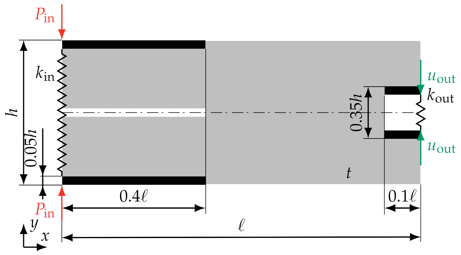
| Input force | 50 | N | |
| Length | ℓ | 200 | mm |
| Height | h | 80 | mm |
| Thickness | t | 5 | mm |
| Input stiffness | 1.5 | N/mm | |
| Output stiffness | 4 | N/mm | |
| Filter radius | 4.7 | mm | |
| Volume fraction | 0.3 | − |
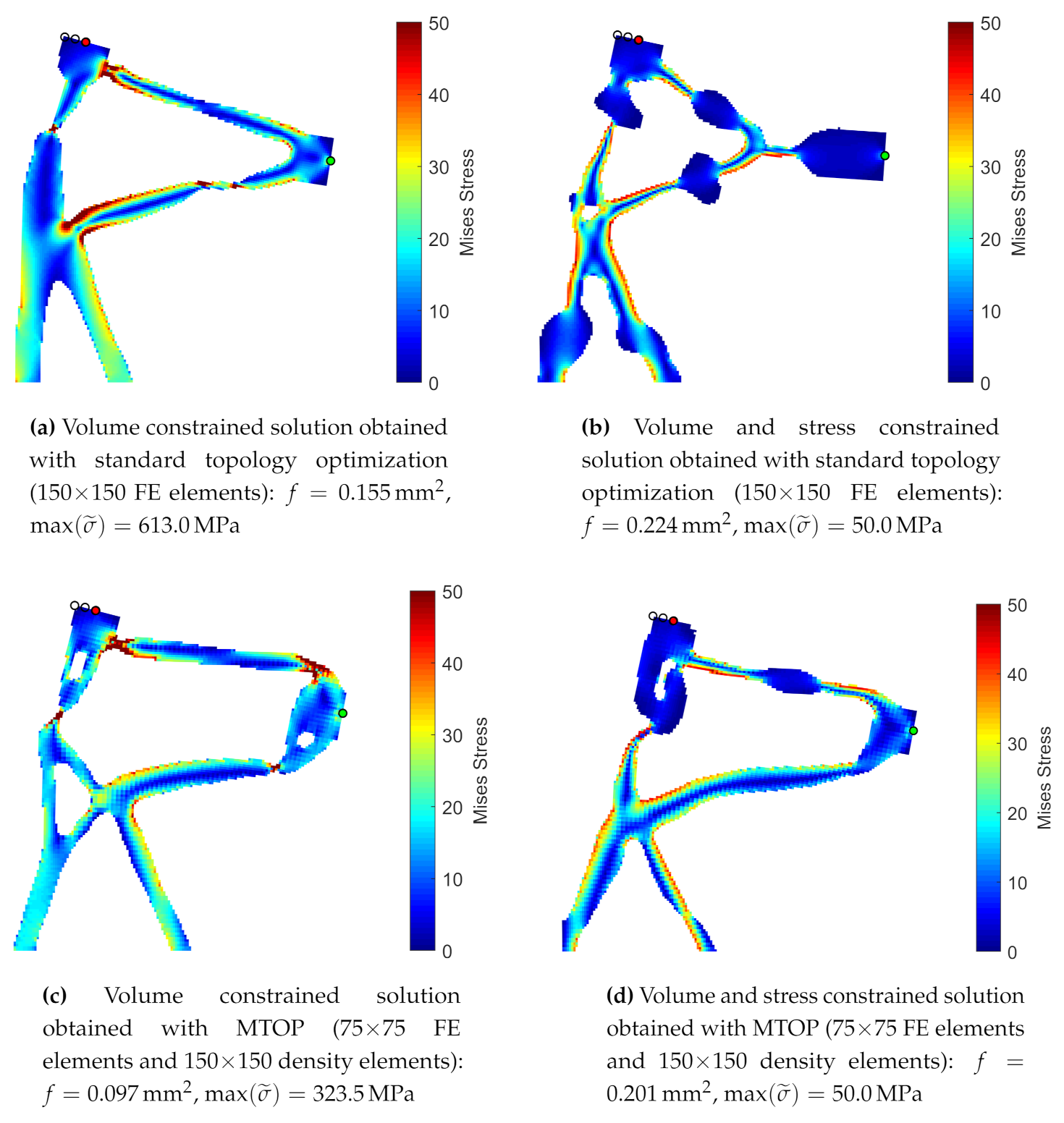
| Solution Topology | Validation Analysis Type | [mm] | [MPa] |
|---|---|---|---|
| a (Figure 3a) | linear nonlinear | 9.76 7.23 | 528.28 624.65 |
| b (Figure 3b) | linear nonlinear | 7.55 5.53 | 49.37 173.74 |
| c (Figure 3c) | nonlinear | 7.84 | 571.28 |
| d (Figure 3d) | nonlinear | 4.27 | 49.95 |
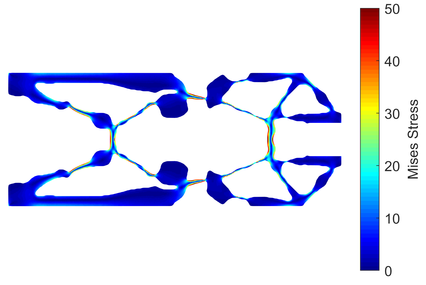
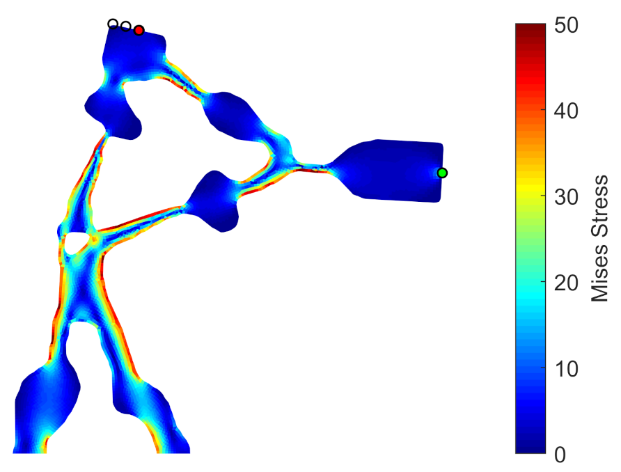
| e (Figure 4) | nonlinear | 4.50 | 51.99 |
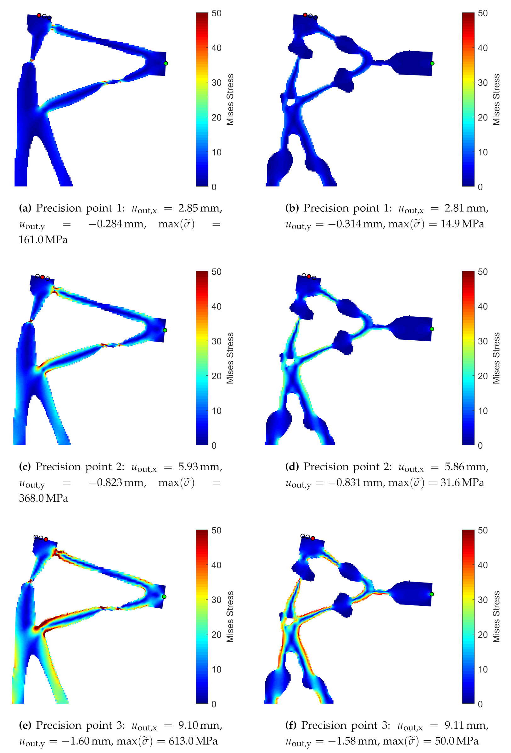
| Precision Point j | [mm] | [mm] | [mm] |
|---|---|---|---|
| 1 | 1.5 | 3 | −0.18 |
| 2 | 3 | 6 | −0.73 |
| 3 | 4.5 | 9 | −1.67 |
| Load Case i | [-] | [N] | [N] |
|---|---|---|---|
| 0 | 1 | 0 | 0 |
| 1 | 0.1 | 40 | 40 |
| 2 | 0.1 | -40 | 40 |
| Precision Point j | [mm] | [mm] | [mm] |
|---|---|---|---|
| 1 | 4 | 5.53 | -14.18 |
| Load Case i | [-] | [N] | [N] |
|---|---|---|---|
| 0 | 1 | 0 | 0 |
| 1 | 0.1 | 14.2 | 32.8 |
Publisher’s Note: MDPI stays neutral with regard to jurisdictional claims in published maps and institutional affiliations. |
© 2021 by the authors. Licensee MDPI, Basel, Switzerland. This article is an open access article distributed under the terms and conditions of the Creative Commons Attribution (CC BY) license (http://creativecommons.org/licenses/by/4.0/).
Share and Cite
Reinisch, J.; Wehrle, E.; Achleitner, J. Multiresolution Topology Optimization of Large-Deformation Path-Generation Compliant Mechanisms with Stress Constraints. Appl. Sci. 2021, 11, 2479. https://doi.org/10.3390/app11062479
Reinisch J, Wehrle E, Achleitner J. Multiresolution Topology Optimization of Large-Deformation Path-Generation Compliant Mechanisms with Stress Constraints. Applied Sciences. 2021; 11(6):2479. https://doi.org/10.3390/app11062479
Chicago/Turabian StyleReinisch, Joseph, Erich Wehrle, and Johannes Achleitner. 2021. "Multiresolution Topology Optimization of Large-Deformation Path-Generation Compliant Mechanisms with Stress Constraints" Applied Sciences 11, no. 6: 2479. https://doi.org/10.3390/app11062479