Article

A New Switching Adaptive Fuzzy Controller with an Application to Vibration Control of a Vehicle Seat Suspension Subjected to Disturbances

1
Department of Mechatronics and Sensor Systems Technology, Vietnamese-German University, Binh Duong 75100, Vietnam
2
School of Electronics, Electrical Engineering and Computer Science, Queen’s University Belfast, Belfast BT7 1NN, UK
3
Department of Mechanical Engineering, The State University of New York, Korea (SUNY Korea), Incheon 21985, Korea
*
Authors to whom correspondence should be addressed.
Appl. Sci. 2021, 11(5), 2244; https://doi.org/10.3390/app11052244
Submission received: 5 February 2021 / Revised: 26 February 2021 / Accepted: 26 February 2021 / Published: 3 March 2021
(This article belongs to the Collection The Development and Application of Fuzzy Logic)

Abstract

:
This paper proposes a new switching adaptive fuzzy controller and applies it to vibration control of a vehicle seat suspension equipped with a semi-active magnetorheological (MR) damper. The proposed control system consists of three functioned filters: (1) Filter 1: a model of interval type 2 fuzzy to compensate disturbances; (2) Filter 2: a ‘switching term’ to evaluate the magnitude of disturbance; and (3) Filter 3: a group of adaptation laws to enhance the robustness of control input. These filters play a role of powerful shields to improve control performance and guarantee the stability of the applied system subjected to external disturbances. After embedding a PID (proportional-integral-derivative) model into Riccati-like equation, main control parameters are updated based on the adaptation laws. The proposed controller is then synthesized in two different cases: high disturbance and small disturbance. For the high disturbance, a special type of sliding surface function, which relates to an exponential function and its t-norm, is used to increase the energy of control system. For the small disturbance, the energy from the modified t-norm of the sliding surface is neglected to reduce the energy consumption with maintaining the desired performance. To demonstrate the effectiveness of the proposed controller, a vehicle seat suspension installed with controllable MR damper is adopted to reflect the robustness against external disturbances corresponding to road excitations. It is validated from computer simulation that the proposed controller can provide better vibration control performance than other existing robust controllers showing excellent control stability with well-reduced displacement and velocity at the position of the seat.

1. Introduction

Modern intelligent controls remain as the ‘heart’ of many devices, especially in industrial machines, automobiles, home appliances, robotics, etc. In this research, due to the flexibility in handling the disturbances, the adaptive control is chosen as a powerful tool in the development of the intelligent controllers. A composite adaptive control for robotic was presented in [1] in which the controller used the lower-bounded matrices of the predicted errors to develop the adaptation laws. Adaptive control with fuzzy model for tracking control was studied in [2] where the tan-type barrier Lyapunov (TBL in short) function was used for the design of the adaptive laws showing better control performance than the log-type BL. Prescribed performance was used to design adaptive control with command-filter in [3] in which the finite time method was applied as main tool for the filter. To enhance the robustness of the controller, a fuzzy system is frequently employed to approximate the unknown linear function. The prescribed performance was embedded into an adaptive fuzzy control in [4] presenting a new transformed error function-based arc-tanh-type function. This function was an inverse hyperbolic tangent function and set following the arc-tanh function to improve its performance. An application of the sliding mode control for the design of adaptive control was presented in [5] where an integral sliding mode controller coupled with a dual-layer adaptive scheme was utilized. A decoupling control using adaptive fuzzy model was developed in [6] in which the main function related to the main control input was analyzed to the second element. Another control methodology used in the design of adaptive model is PID (proportional-integral-derivative) controller. A hybrid PID control integrating with the genetic algorithm and particle swarm optimization was presented in [7]. However, because of large number of iterations, the proposed control proposed in [7] has large time delay in practice. A combination between interval type 2 fuzzy (IT2F in short) model and PID control was described in [8] where the role of IT2F was a feedforward term to compensate the uncertainties and nonlinearities of the system in the design of PID controller. In this work, grey wolf (GW) optimizer and artificial bee colony algorithm were used for automatically turning the parameters of PID. The neural PID control was presented in [9] for minimizing the steady-state error in which the traditional neural PD control was transformed into a new model of neural PID control to compensate the uncertainties. A new adaptive law was developed to adapt the three main parameters of the PID controller considering the signal of dynamic variables of the system [10], and a neural model associated PID controller was also investigated for designing adaptive control laws [11].
It is well known that the classical type of PID model is still an important tool in the design of modern controllers [12]. However, the use of PID-based controller only may cause the lack of robustness against system uncertainties and disturbances. A new form of combination among fuzzy model, adaptive control, sliding mode control and PID model was presented in [13] in which a new form of PID-terminal sliding surface was proposed using the adaptive fuzzy logic to tune the parameters of the PID gains. An adaptive PID controller where the adaptation laws include both the hybrid function error and the gains of the PID controller was also presented in [14]. A composite controller including adaptive control, sliding mode control, PID and fuzzy model was studied in [15] in which a new modified Riccati-like equation and PID model were adopted to control severe disturbances. A new model of adaptive control with prescribed performance of the sliding surface was presented in [16] so that system state variables are to be stayed within the defined boundaries. A new form of adaptive control with optimal control was also investigated in [17] to improve time convergence of the prescribed performance. An adaptive control with PI model was developed in [18] considering Riccati-like equation, sliding mode control and fuzzy model to enhance control robustness. It is evident from the above literature survey that adaptive control remains as a potential controller for various dynamic systems. In addition, the adaptive control can be easily combined with other control types such as sliding mode control, optimal control, fuzzy model and PID model for improving control robustness of many systems subjected to parameter uncertainty and external disturbance.
Consequently, the main technical contribution of this work is to formulate a new robust adaptive controller which preserves merits of PID and fuzzy models, sliding mode control and prescribed performance. More specifically, the following contents are to be carried out in this work: (1) a new integration of conventional sliding surface and prescribed sliding surface for switching control is presented, (2) a novel modified Riccati-like equation with PID parameters is proposed for the design of a new robust control input, (3) a new selection methodology for system constraints adaptable to the change of magnitude of disturbance coupled with dynamic motion is proposed and (4) computer simulations are undertaken to validate the robust stability considering the vibration problem of a vehicle seat suspension equipped with a semi-active magnetorheological (MR) dampers. In the presentation of control performances, a comparison between the proposed controller and two other existing controllers is made to demonstrate some salient properties of the proposed controller showing less vibration magnitude and higher stability against external disturbances (road excitations).
This article is organized as follows. After addressing the research background and motivation in Introduction, design procedures for the proposed controller are presented in Section 2 considering the robustness of input control. In Section 3, computer simulations are carried out for three controllers: the proposed controller and two compared existing controllers. After discussing on vibration control performances of three controllers, the conclusion is drawn in Section 4 validating that the proposed controller can provide better control performance with higher robustness against severe disturbances than two compared controllers.

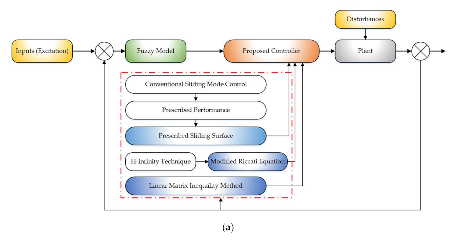
2. Design of a New Adaptive Fuzzy Controller

2.1. Robustness of Input Controls

In the proposed control, the fuzzy model is applied as the first module. The fuzzy model is well explained in [15,16,17,18]. Among many types of the fuzzy models, the interval type 2 fuzzy neural networks (IT2FNN) model is chosen in this work. To fasten the calculation progress, the clustering method is used to decrease the volume of data. Then, the rule base of fuzzy model is defined and the jth If-Then rule can be described as follows:
R f j :   If   h 1   is   H f 1 j   and     and   h n   is   H f n j   Then   g   is   a 0 j + i = 1 n a i j h i
where, H f i j ( i = 1 , , n ; j = 1 , , m ) are fuzzy sets, m is the number of rules, and a i j are interval sets. The output is found by:
g f = g l + g r 2 = Ξ l T ξ l f + Ξ r T ξ r f 2
In Equation (2), Ξ l T = [ w 1 l   w 2 l   w 3 l w n l ] and Ξ r T = [ w 1 r   w 2 r   w 3 r w n r ] are the weighting vectors, which symbolize the relation between the rule layer and type-reduction. The weights firing strength vectors in Equation (2) are given by:
ξ l f = [ f _ 1 i = 1 n f _ i f _ 2 i = 1 n f _ i   f _ 3 i = 1 n f _ i   f _ n i = 1 n f _ i ] T   ,   ξ r f = [ f ¯ 1 i = 1 n f ¯ i f ¯ 2 i = 1 n f ¯ i f ¯ 3 i = 1 n f ¯ i   f ¯ n i = 1 n f ¯ i ] T
In this study, the nth system is used which belongs to a single-input single-output (SISO in short) system. The governing equation of the system is defined as follows:
x ˙ = f ( x ) + g ( x ) u ( t ) + d ( t )
where, f ( x ) R n and g ( x ) R n are two unknown non-linear function vectors, u ( t ) R 1 is control input, d ( t ) R n is an external disturbance vector, | d ( t ) | δ d , where the value δ d R n is an upper bound of d ( t ) and x = [ x 1 , x 2 , , x n ] T = [ x 1 , x ˙ 1 , , x 1 ( n 1 ) ] T R n is the state vector. Let a new vector x ˜ be x ˜ = [ x 1   x 2   x 3     x ( n 1 ) ] T . Then, the system (3) can be rewritten as follows:
x ˜ ˙ = S 1 x ˜ + S 2 T s s
In the above,
S 1 = [ 0 1 0 0 0 0 1 0 . . . . k 1 k 2 k 3 k n 1 ] ,   S 2 = [ 0 0 . 1 ]
The tracking error is then defined as e ( t ) = x 1 x d , where x d is the desired value. It is noted that x 1 is the same as x in Equation (4). The second (prescribed) sliding surface is defined as follows [16]:
σ s = φ ˙ + c s φ
In the above, c s > 0 . The constant c s is always positive because its design is derived from the sliding surface of the conventional sliding mode control. It is remarked that coefficients of the conventional sliding surface are positive to guarantee the stability of control system. Then, the derivative of Equation (5) is obtained as follows.
σ ˙ s = φ ¨ + c s φ ˙ = M 1 + M 2 + M 3 ( f ( x ) + g ( x ) u ( t ) + d ( t ) x ¨ d ) + c s φ ˙
In the above, φ ˙ = 1 2 [ λ ˙ + e ˙ ( t ) λ + e ( t ) λ ˙ e ˙ ( t ) λ e ( t ) ] , φ ¨ = M 1 + M 2 + M 3 e ¨ ( t ) , M 1 = λ ¨ ( λ + e ( t ) ) ( λ ˙ + e ˙ ( t ) ) 2 2 ( λ + e ( t ) ) 2 , M 2 = λ ¨ ( λ e ( t ) ) ( λ ˙ e ˙ ( t ) ) 2 2 ( λ e ( t ) ) 2 , M 3 = ( λ + e ( t ) 2 ( λ + e ( t ) ) 2 + λ e ( t ) 2 ( λ e ( t ) ) 2 )
The lumped uncertainty of system is then defined by:
w = M 3 γ ˜ f ξ f + M 3 γ ˜ g ξ g u + M 3 d ( t )
where, γ f = f ( x ) f ( x ) , γ g = g ( x ) g ( x ) ; ξ f , ξ g are two consequent membership values of functions f ( x ) , g ( x ) , respectively. Using Equations (6) and (7), the time derivative of Equation (6) is rewritten as follows:
σ ˙ s = M 1 + M 2 + M 3 f ( x ) + M 3 g ( x ) u ( t ) M 3 x ¨ d + c s φ ˙ + w
The relationship between Equation (8) and IT2FNN model is expressed as follows:
σ ˙ s = M 1 + M 2 + M 3 θ f ξ f + M 3 θ g ξ g u M 3 x ¨ d + c s φ ˙ + w
where,
θ f = a r g   m i n θ f Δ θ f [ s u p x Δ x | f ( x ) f ( x ) | ] , θ g = a r g   m i n θ g Δ θ g [ s u p x Δ x | g ( x ) g ( x ) | ] ,   Δ θ f = { θ f R n , θ f Θ f } , Δ θ g = { θ g R n , θ g Θ g } ,   Δ x = { x R n , x Θ x } .
In the above definitions, Θ f   ,   Θ g ,   Θ x are constant boundaries.
Now, an equivalent controller is determined from Equation (9) based on the assumption σ ˙ s 0 :
u 1 = 1 M 3 θ ^ g ξ g ( M 1 M 2 M 3 θ ^ f ξ f + M 3 x ¨ d c s φ ˙ )
The equivalent control term u 1 cannot stabilize the system because it cannot compensate the error caused from the fuzzy approximation. In fact, the input control u 1 can be considered as the internal energy of the system. In the physical model, related to the potential energy, the derivative (9) must less than or equal zero. When this situation is obtained, the system will be stable. Thus, it can be assumed that the derivative σ ˙ s is approximated to be zero to find the original control energy (10). However, in real control system, the disturbance or uncertainty always exists and continuously attacks the control system. To guarantee the robustness and stability of the system, a first new robust control part u 2 , which is designed as a similar form to PID controller, can be added as follows:
u 2 = 1 M 3 θ ^ g ξ g ( i = 1 n 1 P ( n 1 ) i x i + 1 2 M 3 Γ ξ z x ˜ P S 2 S 2 T P x ˜ T + K P M 3 S 2 T E E T P B P + + K I 0 M 3 S 2 T E E T P B P d t + K D M 3 S 2 T E ˙ E ˙ T P B P )
The value Γ is the adaptive parameter where its boundary is given by Δ Γ = { Γ R , Γ Θ Γ , σ s Γ ξ z ρ } , and Θ Γ is the constant boundary. The matrix P = P T 0 , in which its result is a solution of Riccati-like equation given by:
P S 1 + S 1 T P + Q σ s Γ ξ z P S 2 S 2 T P + ρ P S 2 S 2 T P K P ξ z S 2 T E E T P B P K I ξ z 0 S 2 T E E T P B P d t K D ξ z S 2 T E ˙ E ˙ T P B P = 0
where, σ s Γ ξ z ρ , K P ξ z ρ , K I ξ z ρ , K D ξ z ρ , ρ is the prescribed attenuation level, Q = Q T 0 and ξ z is the consequent membership value of the IT2FNN model. The error vector E is defined as E = [ e ˙ 1 e ˙ 2 ] T = [ x d x x ˙ d x ˙ ] T . When the value ρ = ξ z ( σ s Γ + K P + K I + K D ) satisfied, Riccati-like equation is rewritten by:
P S 1 + S 1 T P + Q = 0
The first robustness control term, u 2 , is not sufficient for controlling the system under disturbance. Hence, a second robustness control term, u 3 , is designed to adapt to two working scenarios, as follows. Now, the governing Equation (1) can be written following state-space form as follows:
x ˙ = f ( x ) + g ( x ) u ( t ) + d ( t ) A P ( x ( t ) , t ) x ( t ) + B P ( x ( t ) , t ) u ( t ) + C p D ( t )
where, A P R n × n , B P R n × m , u R m , C p R n × m , D R m , and C p D ( t ) D s . It is remarked that D s is the boundary related to the disturbance; C p , D are matrix and vector in a form of the state space derived from the governing equation.

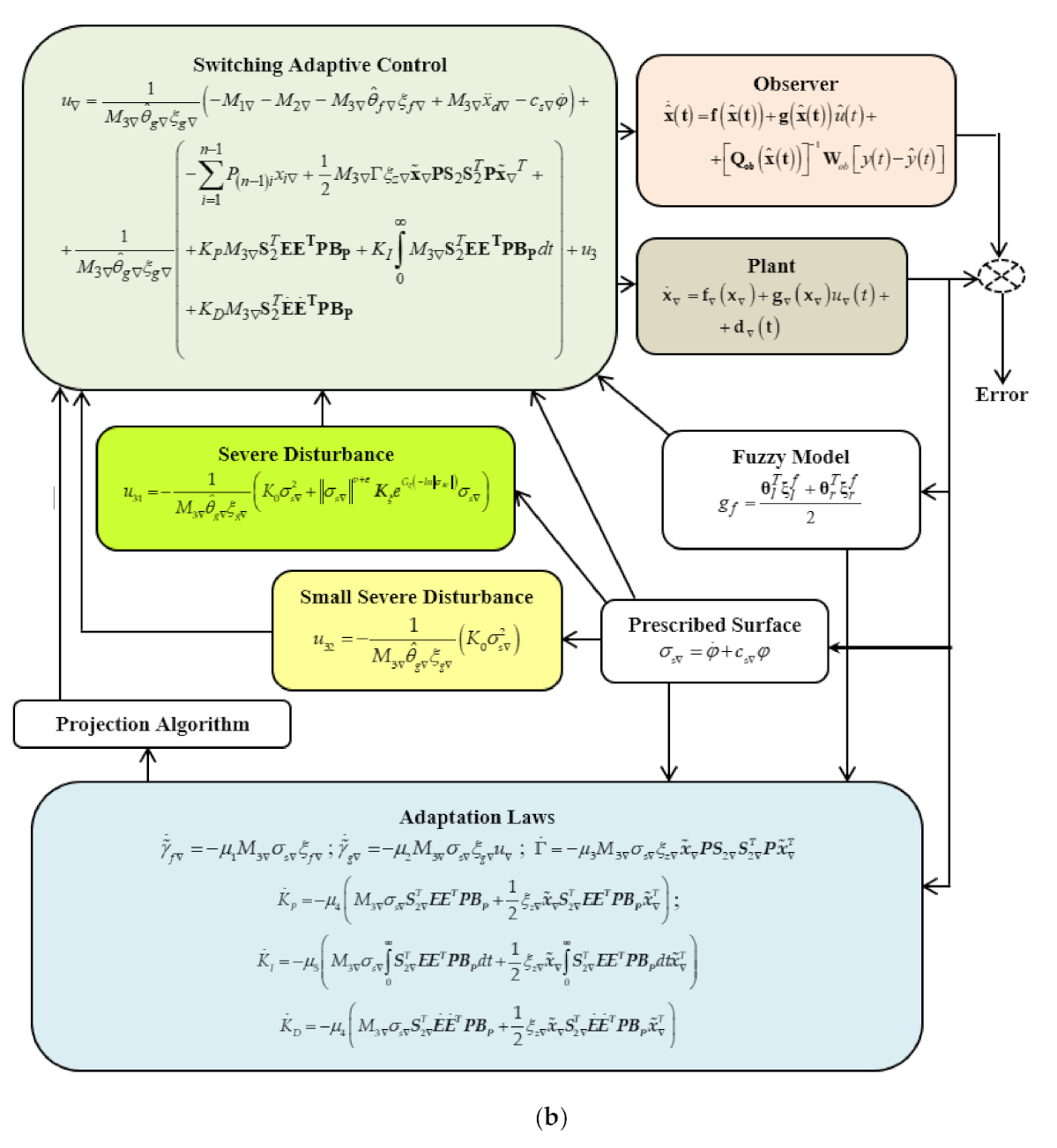
2.2. Formulation of Control Strategy

2.2.1. Proposed Switching Control: High Disturbance Condition

In this case, the disturbance phenomenon generates major effects on the response of the system. Hence, the control input term, u 3 , is proposed as follows:
u 31 = 1 M 3 θ ^ g ξ g ( K 0 σ s 2 + σ s v + ε K ξ e G ξ ( l n σ s ) σ s )
where, K 0 = Z 0 ( γ W I n ) 1 R m × n is a matrix related the properties of the system through the matrices A P and B P ; Z 0 R m × n is a chosen Lyapunov matrix; W R n × n is a matrix which is found from solve the Lyapunov function; γ R , α R + are positive chosen constants; K ξ R m × n is a matrix which is defined as K ξ = Z P ξ ; the matrices Z R m × n and P ξ R n × n are chosen matrices from the constraints system which will be described in next equations; G ξ R n × n is defined as G ξ = v W + ε I n , where I n is the unit matrix; v R , ε R are two positive constants. The value of Z , W , K 0 and K ξ are found from the system constraints which are defined using the linear matrix inequality (LMI in short) method as follows:
[ ( A P W W A P T A P + B P Z 0 ) l n δ d m a x δ d m i n B P Z 0 Z 0 l n δ d m a x δ d m i n l n δ d m a x δ d m i n B P T Z 0 T ( γ W I n ) B P 0 Z 0 l n δ d m a x δ d m i n 0 [ ( A P + B P K 0 ) X + X ( A P + B P K 0 ) T + B P Z + Z T B P T + δ X + D s ] ] 0 ( A P W W A P T A P + B P Z 0 ) ( γ W I n ) B P [ ( A P + B P K 0 ) X + X ( A P + B P K 0 ) T + + B P Z + Z T B P T + δ X + D s ] Z 0 2 l n 2 δ d m a x δ d m i n ( γ W I n ) B P l n δ d m a x δ d m i n [ ( A P + B P K 0 ) X + X ( A P + B P K 0 ) T + + B P Z + Z T B P T + δ X + D s ] 0
where, δ d m i n , δ d m a x are positive robustness parameters which are chosen based on the boundary of disturbance D s and δ d m i n δ d m a x . From the constraint Equation (16), the detailed constraints for the robustness control term are derived and given by:
A P W W A P T A P + B P Z 0 = 0
( γ W I n ) B P < 0
( A P + B P K 0 ) X + X ( A P + B P K 0 ) T + B P Z + Z T B P T + δ X + D s 0
where, X R n × n is chosen matrix; δ R is a positive chosen constant; P ξ = X 1 . The matrix Z 0 R m × n can be found from the solution of Equation (17). The matrix Z R m × n is also found from Equation (19). To prevent the invalid value of the group ( γ W I n ) related to the matrix K 0 , the constant γ is chosen less than 1, and then the group ( γ W I n ) is calculated from the inverse matrix such as 1 / ( γ W I n ) . It is noted that the proof of the proposed LMI (linear matrix inequality) given by Equation (16) can be completed by utilizing Schur’s complement method associated with an appropriated cost function of the system (14).
Remark 1.
The input control (15) is a new design which does not follow the conventional design where the disturbance is assumed to be approximately zero. The Equation (16) with the relations of K 0 , Z 0 , and K ξ will guarantee the stability of the system under disturbance. The constraints Equations (17)–(19) are chosen from the property of Equation (16) which are less than or equal zero. To solve the constraints, the trial-and-error method is used instead of the optimization method because of time-consumption.
Now, the total control u of the system is determined as follows:
u = u 1 + u 2 + u 3
It is noted that the control u 2 is the combination of two sliding surfaces s s and σ s , and PID controller. From the above equations, Equation (9) can be expressed as follows:
σ ˙ s = M 1 + M 2 + M 3 γ ˜ f ξ f + M 3 γ ˜ g ξ g u M 3 x ¨ d + c s φ ˙ + w + M 3 θ ^ f ξ f M 1 M 2 M 3 θ ^ f ξ f + M 3 x ¨ d c s φ ˙ i = 1 n 1 P ( n 1 ) i x i + 1 2 M 3 Γ ξ z x ˜ P S 2 S 2 T P x ˜ T + + K P M 3 S 2 T E E T P B P + K I M 3 0 S 2 T E E T P B P d t + K D M 3 S 2 T E ˙ E ˙ T P B P K 0 σ s 2 σ s v + ε K ξ e G ξ ( l n σ s ) σ s
In the above, γ ˜ f = θ f θ ^ f , γ ˜ g = θ g θ ^ g .
Theorem 1.
The stability and robustness of the proposed control system are guaranteed if the main control function designed by Equations (10), (11) and (15), and the following adaptation laws are utilized.
γ ˜ ˙ f = μ 1 M 3 σ s ξ f
γ ˜ ˙ g = μ 2 M 3 σ s ξ g u
Γ ˙ = μ 3 M 3 σ s ξ z x ˜ P S 2 S 2 T P x ˜ T
K ˙ P = μ 4 ( M 3 σ s S 2 T E E T P B P + 1 2 ξ z x ˜ S 2 T E E T P B P x ˜ T )
K ˙ I = μ 5 ( M 3 σ s 0 S 2 T E E T P B P d t + 1 2 ξ z x ˜ 0 S 2 T E E T P B P d t x ˜ T )
K ˙ D = μ 4 ( M 3 σ s S 2 T E ˙ E ˙ T P B P + 1 2 ξ z x ˜ S 2 T E ˙ E ˙ T P B P x ˜ T )
The proof of Theorem 1 is given in Appendix A. It is noted here that to estimate the states of the system, the conventional Luenberger observer [19] has been used in this work.

2.2.2. Proposed Switching Control: Small Disturbance Condition

When the disturbance phenomenon has small effects on the response of the system, the following control u 3 is proposed.
u 32 = 1 M 3 θ ^ g ξ g ( K 0 σ s 2 )
where, K 0 = Z 0 ( W ( γ + 1 ) I n ) 1 , Z 0 R m × n , W R n × n with the system constraints are defined as follows:
A P W W A P T A P + B P Z 0 = 0
( A P + B P K 0 ) X + X ( A P + B P K 0 ) T + B P Z + Z T B P T + δ X 0
It is noted that constraints (29) and (30) can also be derived by using the Schur’s complement method like the Equation (16). Using Equations (20) and (21) with a new updated control (28), the following equation is obtained.
σ ˙ s = M 1 + M 2 + M 3 γ ˜ f ξ f + M 3 γ ˜ g ξ g u M 3 x ¨ d + c s φ ˙ + w + M 3 θ ^ f ξ f M 1 M 2 M 3 θ ^ f ξ f + M 3 x ¨ d c s φ ˙ i = 1 n 1 P ( n 1 ) i x i + 1 2 M 3 Γ ξ z x ˜ P S 2 S 2 T P x ˜ T + + K P M 3 S 2 T E E T P B P + K I M 3 0 S 2 T E E T P B P d t + K D M 3 S 2 T E ˙ E ˙ T P B P K 0 σ s 2
Theorem 2.
The stability and robustness of the proposed control system are guaranteed if the main control function is designed by Equations (10), (11) and (28), and the adaptation laws are suggested like Equations (22)–(27). The proof of Theorem 2 can be completed using the same approach as the proof of Theorem 1 shown in Appendix A.
Remark 2.
Definition for probability of switching system was shown in [20]. For all Ω p ( 0 , 1 ) , there is a class κ function ( . ) such that C > 0 , t t 0 , | x ( t 0 ) | ( C )
P ( | x ( t ) | C ) 1 Ω p
The value ( C ) is chosen based on the dynamic property of the system. Normally, it is chosen following maximal displacement/or vibration. The group C is also belonged to the dynamic parameters system. The value Ω p is defaulted as 0.2 for small vibration, and 1 for large vibration. This remark will be used for the switching control.
Remark 3.
The fuzzy model-based controller in [21] did not consider disturbance removal in control design process and hence its robustness could not be guaranteed in severe disturbance case. On the contrary, the proposed controller (15) associated with LMI (16) shows a close relationship with the parameters of the system and hence directly solves the disturbance following the desired boundaries. It is noteworthy that the prescribed performance in the sliding surface (5) also can improve the response of the system in case of the boundaries are not found exactly.
Remark 4.
The similar LMI used in the controller [21] has been applied in [22] where the fuzzy model is independent with the LMI whose role is to adjust control gains. Therefore, this controller could not bring robust control and then the convergence time to obtain stable states is long as shown in [22]. As mentioned in Remark 3, the controller proposed in this study combines the conventional sliding surface and the prescribed sliding surface to achieve control robustness, which guarantees the convergence time and anti-affection of the disturbance or uncertainty of the system.

2.2.3. Switching Condition

The third robust control input u 3 of both high disturbances and small disturbances is defined by the following switching condition:
u 3 = { u 31 u 32 i f   | x ¨ ( t ) | max [ x ¨ ( t ) 0 max ]   a n d   | x ( t 0 ) | ( C ) f   | x ¨ ( t ) | < max [ x ¨ ( t ) 0 max ]   a n d   | x ( t 0 ) | < ( C )
The block diagram of all elements related to the control design proposed in this work is shown in Figure 1. The proposed controller shown in Figure 1a includes three main elements: prescribed sliding surface, modified Riccati equation and LMI method. The fuzzy model supports the evaluation of the inputs and feedback signals. It is remarked that the feedback signal is also used as the input of the elements in the proposed controller. The control process of the proposed controller is shown in Figure 1b. Depending on the properties of the disturbance system, the switching control u 31 or u 32 will be chosen for u 3 . The output of the prescribed surface of the new modified sliding mode control will be used as the input of the switching control and adaptation laws. At every single step in the loop, the output of the system is continuously used as the input for the fuzzy model, main control, prescribed sliding surface and adaptation laws. It is remarked that the switching index symbolizing for the choice of control u 3 is established based on conditions given by Equation (33).

3. Simulations for Control Performances

3.1. Dynamic Model and Parameters

In this work, a vehicle seat suspension with MR damper studied in [23] is adopted to demonstrate the effectiveness of the proposed controller for the robust control performance against disturbances. Figure 2 shows a 2-DOF (degrees of freedom) model of the vehicle seat suspension equipped with MR damper where its damping force is represented by FMR (N). The other variables are defined as follows: m1 is the mass of driver (or passenger), m1 = 77 (kg); k1 is the stiffness coefficient of torso k1 = 49.340 (N/m), c1 is the damping coefficient of torso, c1 = 2475 (N.s/m); ms is the mass of the seat, ms = 27 (kg); ks is the stiffness coefficient of the frame, ks = 17.830 (N/m); cs is the damping coefficient of the frame, c s= 1500 (N.s/m); x1 is the displacement of the driver (m), xs is the displacement of the seat (m), x0 is the displacement related excitation (m). More details on this model are given in [17,23].
The dynamic motion equations of the seat suspension system are obtained as follows.
m s x ¨ s = k s ( x s x 0 ) c s ( x ˙ s x ˙ 0 ) + k 1 ( x 1 x s ) + c 1 ( x ˙ 1 x ˙ s ) + F M R
m 1 x ¨ 1 = k 1 ( x 1 x s ) + c 1 ( x ˙ 1 x ˙ s )
The state-space form of Equations (34) and (35) is rewritten as follows.
x ˙ 11 = x ˙ s = x 22 x ˙ 22 = f 11 ( x 11 , x 22 , x 33 , x 44 ) + g 11 ( x 11 , x 22 , x 33 , x 44 ) u x ˙ 33 = x ˙ 1 = x 44 x ˙ 44 = f 22 ( x 11 , x 22 , x 33 , x 44 )
In the above,
f 11 ( x 11 , x 22 , x 33 , x 44 ) = k s m s ( x 11 x 0 ) c s m s ( x 22 x ˙ 0 ) + k 1 m s ( x 33 x 11 ) + c 1 m s ( x 44 x 22 ) , g 11 ( x 11 , x 22 , x 33 , x 44 ) = 1 m s ,   u = F M R ,   f 22 ( x 11 , x 22 , x 33 , x 44 ) = k 1 m 1 ( x 33 x 11 ) c 1 m 1 ( x 44 x 22 )
It is noted that x 11 , x 22 , x 33 , x 44 are variables related to x s and x 1 of the system which are pointed out in both Figure 2 and Equation (36). The value of u = F M R is converted to the input signal to generate the magnetic field for MR damper. This can be solved by using the following equation [23].
F M R = ( c a + c b V ) ( x 44 x 22 ) + k 0 ( x 33 x 11 ) + ( α a + α b V )
Thus, the voltage to be applied to MR damper is found from Equation (37) as follows:
V = F M R [ c a ( x 44 x 22 ) + k 0 ( x 33 x 11 ) + α a ϕ ] c b ( x 44 x 22 ) + α b ϕ
In the above, k 0 is the linear spring stiffness, k 0 = 0 (N/m), ca is the viscous damping coefficient, c a = 990 (N·s/m); c b is the viscous damping coefficient influenced by V, c b = 3.095 (Ns/m V); α a is the stiffness with non-voltage, α a = 545 (N/m); α b is the stiffness influenced by voltage V, α b = 620 (N/m V); ϕ is the positive parameter of hysteresis loop, ϕ = 4. It is noted that the voltage V is directly related to the damping force of MR damper [23].
In this work, computer simulation is carried out with three controllers: the proposed controller, Compared Controller 1 [23], and Compared Controller 2 [24]. The compared controllers are chosen based on its similarity of control structure [23] and switching control logic [24]. In this simulation study, the input excitation force of the model is chosen as similar properties to real conditions, which have complicated road disturbances. The random step wave road and bump road shown in Figure 3 are used. Control parameters for three controllers used in this simulation are given in Table 1, Table 2 and Table 3. These values are appropriately chosen based on both the real seat suspension of a passenger car and the maximum damping force of MR damper [23]. It is noted that in the Compared Controller 1, the equations for coding program include Equations (14) and (15) and adaptation laws Equations (20)–(27), while in the Compared Controller 2, the Equations (14) and (28) and adaptation laws Equations (20)–(27) are used for coding program.

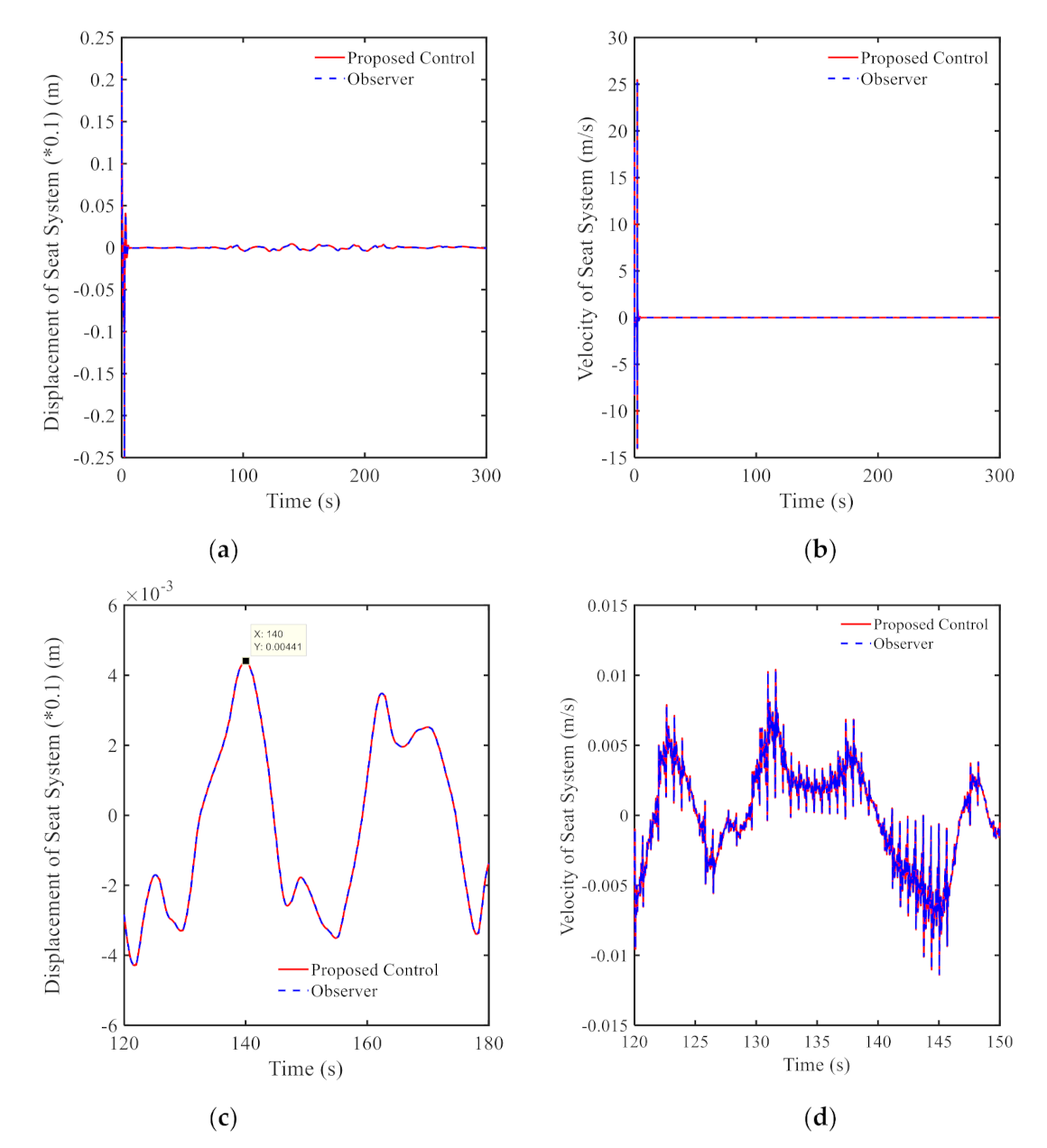
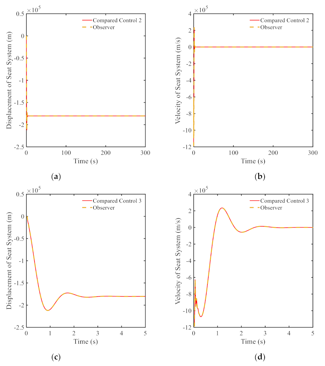
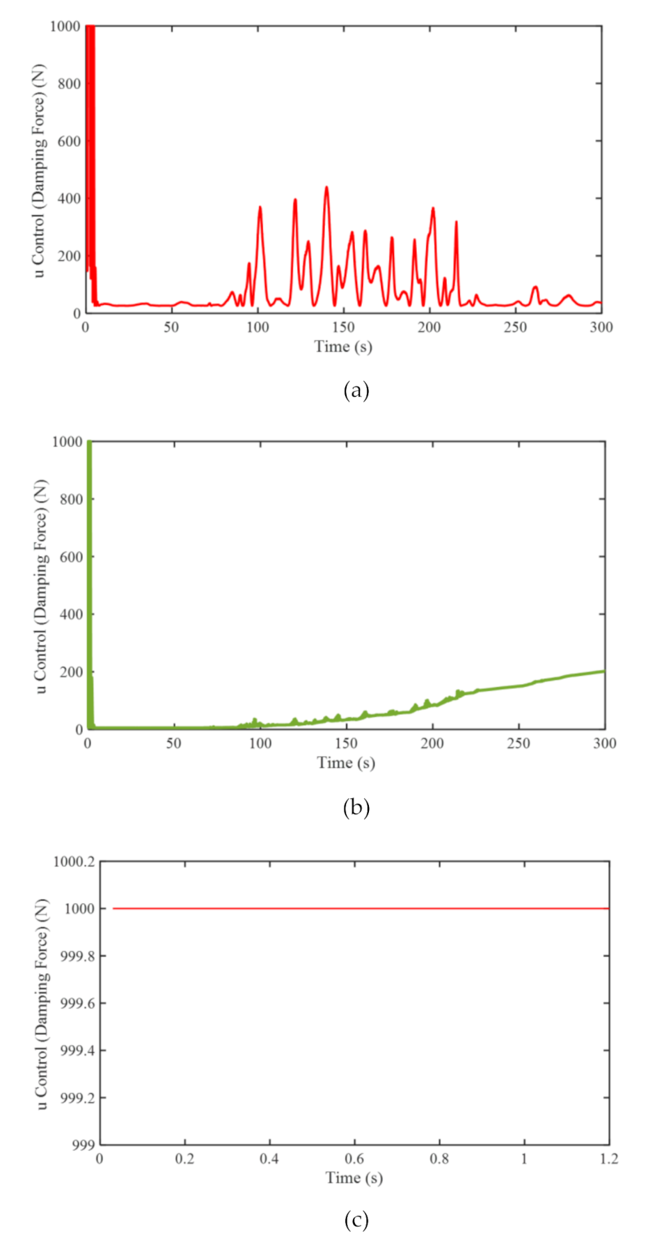
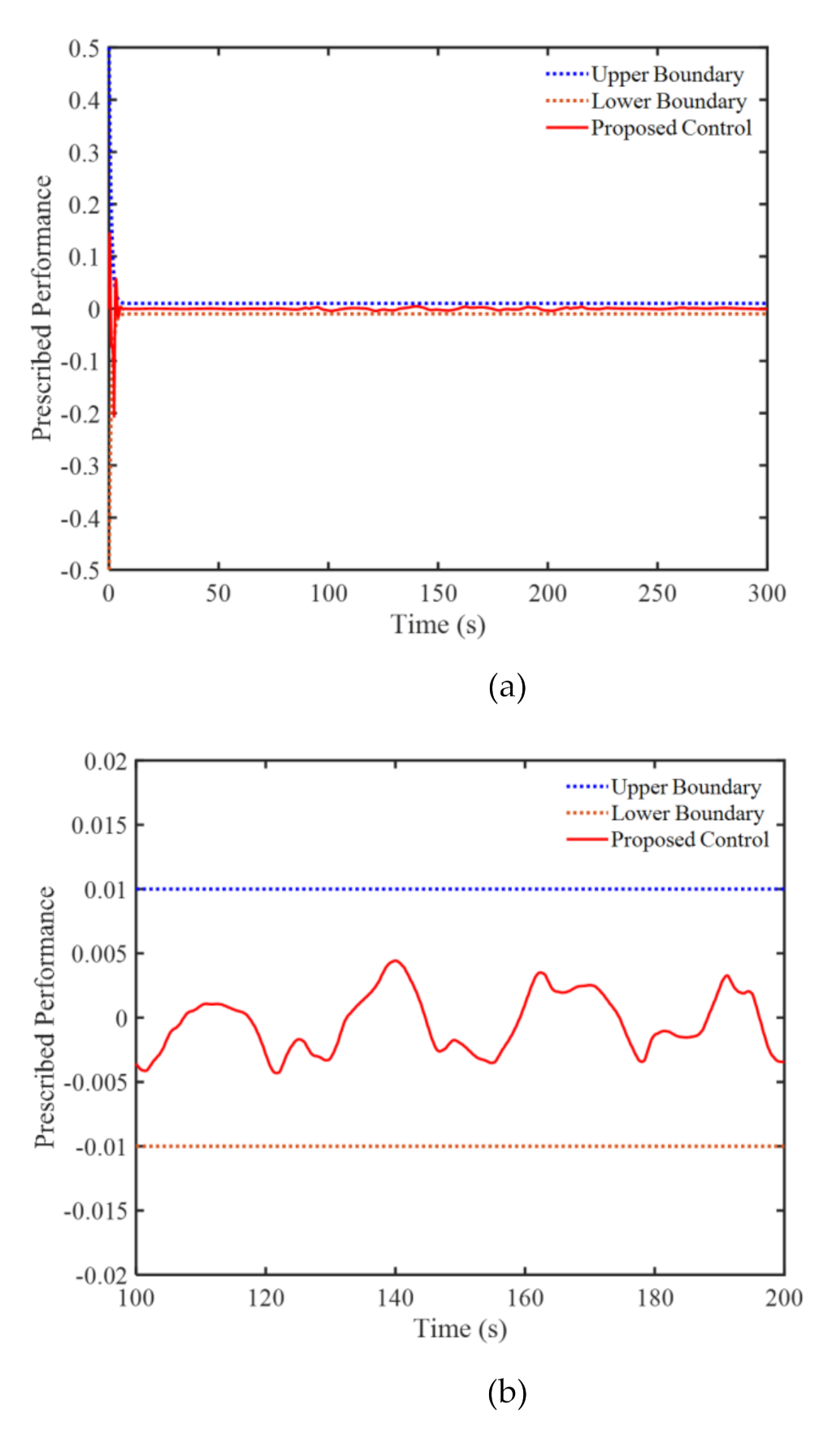
3.2. Results and Discussions

The purpose of the simulation is to prove the robustness of the proposed controller. To achieve this goal, both the displacement and velocity at the seat position subjected to road excitation are investigated and compared with two existing controllers; Compared Controller 1 and Compared Controller 2. Figure 4, Figure 5 and Figure 6 present vibration control performance of the proposed controller, Compared Controller 1 and Compared Controller 2, respectively. In the results, (a) and (b) represent control responses for a few minutes motion, while (c) and (c) represent control performance for one minute to observe more detailed profiles of the displacement and velocity components at the seat position. It is clearly seen from the results that the proposed controller provides the best vibration control performance in terms of the magnitudes of the displacement and velocity. Specifically, the maximum peak of the displacement is identified by 0.00441 (m) by activating the proposed controller, while it is extremely high in the Compared Controllers 1 and 2. It is also understood from the signal profiles of the enlarged view (d) that both the proposed controller and Compared Controller 1 follow the model of adaptive fuzzy PID control showing the switching motion. This behavior can be expected from both the prescribed sliding surface and the choice of robustness function, given by Equations (15) and (28), respectively. On the other hand, it is clearly seen from the results of Compared Controller 2 that vibration control performance is not good exhibiting unstable motion. In fact, the constraints functions in the input control of the Compared Controller 2 are not sufficient to capture the control energy to overcome the imposed disturbance.
Figure 7 presents control input which corresponds to the damping force generated from MR damper by each controller. It is clearly seen that the control input of the proposed controller has been well applied to the system with the switching logic associated with the prescribed sliding surface. In other words, the variation of energy is changed in the proposed controller following the magnitude of the excitation. In addition, it is identified that the energy consumption of the proposed controller is less than the Compared Controllers 1 and 2. To analyze the robustness of the proposed controller associated with the switching logic, both the prescribed performance and switching index are shown in Figure 8 and Figure 9. It is identified from Figure 8a that the values of the proposed controller always belong to the setup boundaries of the prescribed model shown in Figure 8b. The switching index of the switching control functions is shown in Figure 9. This figure indicates that the switching function of the proposed controller is efficient to reject the disturbances with the fast response time. This result also shows the variation of the switching function (33), which points out the change of the input control taking account for the magnitude of disturbance. In Figure 9, the index value 1 indicates the state with high disturbance, while the index value 0.2 denotes the small disturbance. It is noteworthy that the symmetric state in control with the switching index is clearly viewed in Figure 7a. In addition, it is noted that the minimum value of damping force shown in Figure 7a is not zero. This value indicates the switching function (34) calculated from Equations (15) and (28). The results shown in this section are quite self-explanatory justifying that the proposed adaptive fuzzy controller can be effectively applied to several control systems subjected to severe external disturbances.

4. Conclusions

In this study, a new switching adaptive controller was proposed and applied to vibration control of a semi-active vehicle seat suspension system featuring MR damper. To formulate the switching controller, the interval type 2 fuzzy model was used. Basically, the proposed controller has two sliding surfaces: one is conventional surface for the initial states of the system and the other is the prescribed surface for the objective performance. Based on these two sliding surfaces, the main input of the equivalent controller and robust controller were separately designed and combined to ensure the stability and robustness against disturbances. In the design of the proposed controller, adaptation laws were determined based on Lyapunov stability. In order to demonstrate the effectiveness of the proposed controller, two other existing controllers were adopted from the references and their vibration control performances were compared. From the comparative investigation, it has been demonstrated that the proposed controller always provides better performance than the compared existing controllers in both high and small disturbance environments.
It is finally remarked that an experimental realization of the proposed controller will be undertaken in near future. In this experimental test, several excitation frequencies mimicking various road conditions are to be seriously considered for the evaluation of the ride comfort of the vehicle seat.

Author Contributions

Conceptualization and methodology, D.X.P. and S.-B.C.; computer simulation and data curation, D.X.P. and V.M.; original draft preparation and writing, D.X.P.; review and editing, S.-B.C.; supervision, S.-B.C. All authors have read and agreed to the published version of the manuscript.

Funding

This research was funded by Vietnam National Foundation for Science and Technology Development (NAFOSTED) under grant number 107.02-2020.13. The APC was funded by Prof. Seung-Bok Choi (The State University of New York at Korea).

Institutional Review Board Statement

Not applicable.

Informed Consent Statement

Not applicable.

Data Availability Statement

Not applicable.

Conflicts of Interest

The authors declare that there are no conflicts of interest.

Appendix A

Proof of Theorem 1.
To prove the above theorem, a Lyapunov function candidate is proposed as follows:
L = 1 2 σ s 2 + 1 2 x ˜ P x ˜ T + 1 2 μ 1 γ ˜ 2 f + 1 2 μ 2 γ ˜ 2 g + 1 2 μ 3 Γ 2 + 1 2 μ 4 K P 2 + 1 2 μ 5 K I 2 + 1 2 μ 6 K D 2
The derivative of Equation (A1) with respect to time is obtained as:
L ˙ = σ s σ ˙ s + 1 2 x ˜ ˙ P x ˜ T + 1 2 x ˜ P x ˜ ˙ T + 1 μ 1 γ ˜ f γ ˜ ˙ f + 1 μ 2 γ ˜ g γ ˜ ˙ g + 1 μ 3 Γ Γ ˙ + 1 μ 4 K P K ˙ P + + 1 μ 5 K I K ˙ I + 1 μ 6 K D K ˙ D
Substituting Equation (21) into Equation (A2) yields the following.
L ˙ = [ M 3 σ s γ ˜ f ξ f + 1 μ 1 γ ˜ f γ ˜ ˙ f ] + [ M 3 σ s γ ˜ g ξ g u + 1 μ 2 γ ˜ g γ ˜ ˙ g ] + +   [ M 3 Δ Γ ξ z σ s x ˜ P S 2 S 2 T P x ˜ T + 1 μ 3 Γ Γ ˙ ] + [ K P M 3 S 2 T E E T P B P + 1 2 K P ξ z x ˜ S 2 T E E T P B P x ˜ T + + 1 μ 4 K P K ˙ P ] + + [ K I M 3 0 S 2 T E E T P B P d t + 1 2 K I ξ z x ˜ 0 S 2 T E E T P B P d t x ˜ T + 1 μ 5 K I K ˙ I ] + + [ K D M 3 S 2 T E ˙ E ˙ T P B P + 1 2 K D ξ z x ˜ S 2 T E ˙ E ˙ T P B P x ˜ T + 1 μ 6 K D K ˙ D ] + + [ σ s w ( K 0 σ s 3 + σ s v + ε K ξ e G ξ ( l n σ s ) σ s 2 ) 1 2 ρ x ˜ P S 2 S 2 T P x ˜ T 1 2 x ˜ Q x ˜ T ]
It is noted that Equation (20) is used in finding Equation (A3). Now, substituting Equations (22)–(27) into Equation (A3) yields the following.
L ˙ σ s w ( K 0 σ s 2 + σ s v + ε K ξ e G ξ ( l n σ s ) σ s ) 1 2 ρ x ˜ P S 2 S 2 T P x ˜ T 1 2 x ˜ Q x ˜ T   [ 1 2 x ˜ Q x ˜ T ( K 0 σ s w K 0 ) 2 + w 2 K 0 ] 1 2 ρ x ˜ P S 2 S 2 T P x ˜ T 1 2 x ˜ Q x ˜ T + w 2 K 0
The above equation cannot be used for the conclusion of stability. Hence, it needs to be integrated from t = 0 to t = T ;
L ( 0 ) L ( T ) + 1 K 0 0 T w 2 d t 1 2 0 T x ˜ Q x ˜ T d t
where,
L ( 0 ) = 1 2 σ s 2 ( 0 ) + 1 2 x ˜ ( 0 ) P x ˜ T ( 0 ) + 1 2 μ 1 γ ˜ 2 f ( 0 ) + 1 2 μ 2 γ ˜ 2 g ( 0 ) + 1 2 μ 3 Γ 2 ( 0 ) + 1 2 μ 4 K P 2 ( 0 ) + + 1 2 μ 5 K I 2 ( 0 ) + 1 2 μ 6 K D 2 ( 0 )
The value L ( T ) is always positive, and thus Equation (A5) is determined by
L ( 0 ) + 1 K 0 0 T w 2 d t 1 2 0 T x ˜ Q x ˜ T d t 0
This completes the proof. □

References

  1. Li, Y.; Yin, Y.; Zhang, S.; Dong, J.; Johansson, R. Composite adaptive control for bilateral teleoperation systems without persistency of excitation. J. Frankl. Inst. 2020, 357, 773–795. [Google Scholar] [CrossRef] [Green Version]
  2. Zhang, Z.; Wu, Y. Adaptive Fuzzy Tracking Control of Autonomous Underwater Vehicles with Output Constraints. IEEE Trans. Fuzzy Syst. 2020, 1. [Google Scholar] [CrossRef]
  3. Sun, W.; Wu, Y.-Q.; Sun, Z.-Y. Command Filter-Based Finite-Time Adaptive Fuzzy Control for Uncertain Nonlinear Systems With Prescribed Performance. IEEE Trans. Fuzzy Syst. 2020, 28, 3161–3170. [Google Scholar] [CrossRef]
  4. Shi, W. Adaptive Fuzzy Output Feedback Control for Non-Affine MIMO Nonlinear Systems with Prescribed Performance. IEEE Trans. Fuzzy Syst. 2020, 1. [Google Scholar] [CrossRef]
  5. Van, M.; Ge, S.S. Adaptive Fuzzy Integral Sliding Mode Control for Robust Fault Tolerant Control of Robot Manipulators with Disturbance Observer. IEEE Trans. Fuzzy Syst. 2020, 1. [Google Scholar] [CrossRef] [Green Version]
  6. Sun, W.; Lin, J.-W.; Su, S.-F.; Wang, N.; Er, M.J. Reduced Adaptive Fuzzy Decoupling Control for Lower Limb Exoskeleton. IEEE Trans. Cybern. 2021, 51, 1099–1109. [Google Scholar] [CrossRef] [PubMed]
  7. Amiri, M.S.; Ramli, R.; Ibrahim, M.F. Hybrid design of PID controller for four DoF lower limb exoskeleton. Appl. Math. Model. 2019, 72, 17–27. [Google Scholar] [CrossRef]
  8. Gaidhane, P.J.; Nigam, M.J.; Kumar, A.; Pradhan, P.M. Design of interval type-2 fuzzy precompensated PID controller applied to two-dof robotic manipulator with variable payload. ISA Trans. 2019, 89, 169–185. [Google Scholar] [CrossRef]
  9. Yu, W.; Rosen, J. Neural PID Control of Robot Manipulators with Application to an Upper Limb Exoskeleton. IEEE Trans. Cybern. 2013, 43, 673–684. [Google Scholar] [CrossRef]
  10. Sangpet, T.; Kuntanapreeda, S.; Schmidt, R. An adaptive PID-like controller for vibration suppression of piezo-actuated flexible beams. J. Vib. Control. 2017, 24, 2656–2670. [Google Scholar] [CrossRef]
  11. Shojaei, K. Neural adaptive PID formation control of car-like mobile robots without velocity measurements. Adv. Robot. 2017, 31, 947–964. [Google Scholar] [CrossRef]
  12. Su, Y.; Zheng, C. PID control for global finite-time regulation of robotic manipulators. Int. J. Syst. Sci. 2016, 48, 547–558. [Google Scholar] [CrossRef]
  13. Van, M.; Do, X.P.; Mavrovouniotis, M. Self-tuning fuzzy PID-nonsingular fast terminal sliding mode control for robust fault tolerant control of robot manipulators. ISA Trans. 2020, 96, 60–68. [Google Scholar] [CrossRef]
  14. Raaja, G.S.; Vinodh, K.E.; Selvakumar, K.; Vamsi, K.C. Uniform ultimate bounded robust model reference adaptive PID control scheme for visual servoing. J. Frankl. Inst. 2017, 354, 1741–1758. [Google Scholar]
  15. Phu, D.X.; An, J.-H.; Choi, S.-B. A Novel Adaptive PID Controller with Application to Vibration Control of a Semi-Active Vehicle Seat Suspension. Appl. Sci. 2017, 7, 1055. [Google Scholar] [CrossRef]
  16. Phu, D.X.; Huy, T.D.; Mien, V.; Choi, S.-B. A new composite adaptive controller featuring the neural network and prescribed sliding surface with application to vibration control. Mech. Syst. Signal Process. 2018, 107, 409–428. [Google Scholar] [CrossRef]
  17. Do, X.P.; Nguyen, Q.H.; Choi, S.-B. New hybrid optimal controller applied to a vibration control system subjected to severe disturbances. Mech. Syst. Signal Process. 2019, 124, 408–423. [Google Scholar] [CrossRef]
  18. Phu, D.X.; Choi, S.-M.; Choi, S.-B. A new adaptive hybrid controller for vibration control of a vehicle seat suspension featuring MR damper. J. Vib. Control. 2016, 23, 3392–3413. [Google Scholar] [CrossRef]
  19. Ciccarella, G.; Mora, M.D.; Germani, A. A Luenberger-like observer for nonlinear systems. Int. J. Control. 1993, 57, 537–556. [Google Scholar] [CrossRef]
  20. Jiao, T.; Zheng, W.X.; Xu, S. On stability of a class of switched nonlinear systems subject to random disturbances. IEEE Trans. Circuits Syst. I Regul. Pap. 2016, 63, 2278–2289. [Google Scholar] [CrossRef]
  21. Hosseinzadeh, M.; Sadati, N.; Zamani, I. H∞ disturbance attenuation of fuzzy large scale system. In Proceedings of the IEEE International Conference on Fuzzy Systems 2011, Taipei, Taiwan, 27–30 June 2011. [Google Scholar]
  22. Aguiar, C.; Leite, D.; Pereira, D.; Andonovski, G.; Škrjanc, I. Nonlinear modeling and robust LMI fuzzy control of overhead crane systems. J. Frankl. Inst. 2021, 358, 1376–1402. [Google Scholar] [CrossRef]
  23. Do, X.P.; Seung, B.C. A new adaptive fuzzy PID controller based on Riccati-like equation with application to vibration control of vehicle seat suspension. Appl. Sci. 2019, 9, 4540. [Google Scholar]
  24. Zimenko, K.; Polyakov, A.; Efimov, D.; Perruquetti, W. Robust Feedback Stabilization of Linear MIMO Systems Using Generalized Homogenization. IEEE Trans. Autom. Control. 2020, 65, 5429–5436. [Google Scholar] [CrossRef]
Figure 1. Control strategy of the proposed controller: (a) block diagram, (b) control process.
Applsci 11 02244 g001aApplsci 11 02244 g001b
Figure 2. Mechanical model of the vehicle seat suspension with magnetorheological (MR) damper.
Applsci 11 02244 g002
Figure 3. Random step wave road excitation.
Applsci 11 02244 g003
Figure 4. Displacement and velocity of the seat system using the proposed controller: (a,b) general view, (c,d) enlarged view.
Applsci 11 02244 g004
Figure 5. Displacement and velocity of the seat system of the Compared Controller 1: (a,b) general view, (c,d) enlarged view.
Applsci 11 02244 g005aApplsci 11 02244 g005b
Figure 6. Displacement and velocity of seat system of the Compared Controller 2: (a,b) general view, (c,d) enlarged view.
Applsci 11 02244 g006
Figure 7. Damping force control: (a) proposed controller, (b) Compared Controller 1, (c) Compared Controller 2.
Applsci 11 02244 g007
Figure 8. Prescribed performance of the proposed controller: (a) general view, (b) enlarged view.
Applsci 11 02244 g008
Figure 9. Switching index of the proposed controller: (a) general view, (b) enlarged view.
Applsci 11 02244 g009
Table 1. Parameters of the seat suspension for the proposed controller.
ParameterValue
Initial value of prescribed performance λ ( 0 ) 0.5
Infinity value of prescribed performance λ 0.001
Exponential value of prescribed performance l 0.00047
Maximum damping force1000 N
Parameters of sliding surface [ k 1 , k 2 ] [ 1 ,   2 0 ]
Constant of prescribed surface c s 5000
Riccati’s parameter Γ 10
Riccati’s matrix Q [ 2   0 ; 0   2 ]
Observer matrix Q o b [ 1   0 ; 0   1 ]
Observer matrix W o b [ 30 ; 10 ]
Constants of adaptation laws ( μ 1 μ 6 ) 10
Initial state for proposed control [ 0.035 2.5 ]
Initial state for observer [ 0.035 2.5 ]
Robustness parameter γ 0.00001
Robustness parameter v 1
Robustness parameter ε 1
Robustness parameter δ 0.5
Disturbance matrix D s [ 2 2 ; 2 2 ]
Robustness matrix W [ 1 1 ; 1 1 ]
Constant of switching condition ( C ) 0.001 m
Constant of switching condition Ω p 0.8
Acceleration maximum value max [ x ¨ ( t ) 0 max ] 0.01 m/s2
Table 2. Parameters of the seat suspension for Compared Controller 1 [23].
ParameterValue
Parameters of sliding surface [ k 1 , k 2 ] [ 1 ,   0.02 ]
Constant of PID K P 10
Constant of PID K I 150
Constant of PID K D 50
Maximum damping force1000 N
Riccati’s parameter Γ 0.01
Riccati’s matrix Q [ 2   0 ; 0   2 ]
Observer matrix Q 0 [ 1   0 ; 0   1 ]
Observer matrix W 0 [ 30 ; 10 ]
Constants of adaptation laws ( μ 1 μ 6 ) 700
Initial state for proposed control [ 0.035 2.5 ]
Initial state for observer [ 0.035 2.5 ]
Table 3. Parameters of the seat suspension for Compared Controller 2 [24].
ParameterValue
Maximum damping force1000 N
Observer matrix Q 0 [ 1   0 ; 0   1 ]
Observer matrix W 0 [ 30 ; 10 ]
Robustness parameter γ 0.00001
Robustness parameter v 1
Robustness parameter ε 1
Robustness parameter δ 0.1
Robustness vector y 0 [ 67170 3.975.10 3 ]
Robustness matrix L [ 5.10 8 6.10 10 ; 5.10 5 1.10 6 ]
Robustness matrix G d [ 1 1 ; 1 1 ]
Initial state for control [ 0.035 2.5 ]
Initial state for observer [ 0.035 2.5 ]
Publisher’s Note: MDPI stays neutral with regard to jurisdictional claims in published maps and institutional affiliations.

