1. Introduction
The unprecedented increase in demand for remote work, remote teaching and video conferencing has brought a surge not only in network traffic, but unfortunately, in the number of attacks as well. According to [
1], these attacks have surged by 800%. Having reliable, safe and secure functionality of various network services has never been more important.
Cybersecurity covers three different fields: traditional network security, which deals with protecting physical communication links and networking devices; network monitoring and threat detection; and protection against cybercrimes, such as ransomware attacks and identity theft [
2].
1.1. Communication Networks Threats
Attacks on communication networks are increasingly sophisticated such that they even use artificial intelligence (AI) in combination with machine learning and automation. These technologies make attacks faster, broaden their impacts and make them more difficult to detect, especially if masking is used to conceal the attack. Tools for launching AI-based attacks can be easily downloaded, and because their use requires no deep knowledge, such attacks can be initiated by practically anyone. Finally, modern Internet of Things (IoT) devices, which are now widely used in various situations, present a tempting target for attackers. These devices have very limited protection capabilities but often collect sensitive data of very high value.
1.2. AI-Based Cybersecurity
The field of cybersecurity in communication networks has never faced such challenges as those that exist today. Traditional network protections offer only very limited defense against threats utilizing AI [
3]. To combat these attacks, effective protection methods must also utilize AI.
1.2.1. Advantages of AI-Based Protection
Use of AI can significantly increase attack detection rates to nearly 100% when combined with threat intelligence and machine learning [
4]. AI can also provide much better performance in all related functions. According to one survey [
5] that analyzed 603 U.S. organizations, that superiority includes the areas of threat analysis (69%), containment of infected end devices (64%) and identification of application security vulnerabilities (60%). AI is able to cope with the large amounts of relevant data. Moreover, according to the same study, AI in combination with machine learning can detect even previously unknown threats (so-called zero day attacks) with success rates of up to 63%. Finally, AI can reduce labor hours by as much as 75%, especially in the areas of analyzing vulnerabilities, securing networks and reacting to false positive detection [
5].
1.2.2. Disadvantages of AI-Based Protection
AI-based cybersecurity solutions have disadvantages, as well. First, achieving proper functionality requires rigorous training of the AI. Such training can be accomplished only on a large set of clean data. These data have to provide sufficient variability to allow optimal learning. For data to be clean, it must be possible to assume that they contain no unwanted traffic patterns that could be misused by an attacker. This could lead to a so-called AI-proof attack that would not be recognized by the protection solution. Unfortunately, the extent of the data does not allow manual checking and detailed verification of its content.
A second disadvantage consists of the immense demands placed upon computational hardware resources. AI uses demanding algorithms that require considerable capacity. Finally, the initial configuration and subsequent maintenance might require deeper knowledge and more work than do traditional network protection tools.
1.2.3. Summary
In conclusion, there exists a consensus [
6,
7,
8] that AI works best when combined with traditional protection methods and when it is deployed to assist humans but not with the intention of replacing them completely.
1.3. Integration of AI-Based Cybersecurity Protection
The basic approach to integrating an AI-based cybersecurity protection system into a traditional communication network utilizes a dedicated general device, such as a server or networking device, based on traditional x86 CPU architecture and an open UNIX-based operating system. Such a device provides a flexible platform for implementing the system. As networking devices of traditional networks typically use proprietary software and custom hardware, they cannot in this case be used for the system integration.
1.3.1. Software-Defined Networking
Software-defined networking (SDN) is a viable paradigm that combines general networking devices with a software-based controller and allows integration of traditional networking. This concept is based on physical separation of the forwarding plane—which remains on general networking devices—and placing the control plane in the form of a software application (termed an SDN controller) in a dedicated server.
The SDN controller manages all networking functions by delivering instructions to networking devices while providing centralized network management to system operators. The controller can be extended by custom-made applications to achieve a required functionality, such as cybersecurity.
1.3.2. Use of SDN to Integrate AI-Based Protection
The programmability of SDN allows extension of the controller with AI-based protection functionality, as demonstrated in [
9]. This functionality does not require dedicated hardware devices and can be updated at any time. This leads to a more robust and comprehensive solution than does the approach of traditional networks and utilizes dedicated hardware devices and proprietary software [
10]. SDN can be used for all areas of cybersecurity, from anomaly detection to threat mitigation.
1.4. Related Work
State-of-the-art research in the area of AI-based SDN protection can be classified into several fields: anomaly detection, protection against (D)DoS (Distributed Denial of Service), and performance.
1.4.1. Anomaly Detection
The key functionality of a protection system consists of the ability to detect anomalies and to provide effective network monitoring. A large amount of traffic requires the detection to be fully automated. Use of SDN offers a unique advantage in terms of traffic statistics. These statistics are automatically collected on all SDN-enabled networking devices and can be utilized for anomaly detection, as was presented in [
11]. This approach eliminates the need to utilize dedicated devices for performing sampling-based detection, and therefore reduces cost and simplifies the network topology.
Collected statistics can be used to classify data flows and to perform filtering actions, such as blocking the traffic. This was researched in [
12], where the authors developed a framework called ATLANTIC. That framework combined information theory and machine learning to calculate deviations in flow table entropy and to perform automated mitigation.
Collecting statistics on networking devices has two significant limitations. Firstly, the data are aggregated, and secondly, they are available only for lower networking layers (not the application layer). This flaw can be mitigated by forwarding the traffic via the SDN controller. This was demonstrated in the SDN-based firewall developed by Qiumei et al. [
13]. The application layer firewall used supervised machine learning in combination with a typical binary classification problem to filter the traffic. The firewall achieved a relatively high detection accuracy of 96.79% and very low average latency of 0.2 ms.
1.4.2. Protection against (D)DoS
Availability is one of the most important aspects in relation to computer networks. Attacks on availability try to disrupt the service by overwhelming the device or software resources. This makes the service inaccessible for legitimate users. These attacks can be classified into traditional DoS attacks, where only a single attacker is pursuing the attack, and distributed versions ((D)DoS), where the attacker utilizes a large number of devices (often previously compromised devices—so-called zombies) to carry out the attack. Protection against these attacks is very complicated and typically does not provide 100% reliability.
The first step of every protection is to detect the attack. Bhushan et al. [
14] described use of SDN in a cloud environment for this detection with very low communication and computation overheads. A more advanced detection of (D)DoS and port scan attacks was described in [
10]. This solution used a combination of two detection methods: discrete wavelet transform and random forest.
The second step is to take an automated mitigating action, dramatically shortening what would otherwise be a slow response time attainable by human operator. A combination of SDN together with network functions virtualization (NFV) was used for this purpose in [
15]. Those authors used threshold-based classification, and on this basis a filtering action was taken such that the corresponding packets were dropped with a probability ranging from 10% to 100%. Another approach to automated protection was described in [
16]. Those authors developed a framework called ArOMA that integrated traffic monitoring, anomaly detection and mitigation. This solution fully utilized the SDN advantage to integrate all these functions without the need for a dedicated hardware device or installation of specific software.
Efficient detection and mitigation of (D)DoS attacks will be especially important in future large-scale networks integrating IoT devices. As presented by the authors of [
11], utilization of SDN and automatically collected statistics stored on networking devices is more efficient and can achieve greater detection accuracy than traditional sampling-based detection methods.
1.4.3. Performance
SDN is based on software processing, which, by its nature, is always slower than is hardware-accelerated processing of traditional networking devices. On the other hand, SDN provides features that can eliminate slower software processing. This includes proactive insertion of flow rules and use of hardware-accelerated tables for storing and using these rules.
The first issue was analyzed in [
17], where the author determined that use of default reactive insertion of flow rules increases latency by 4 ms in typical network scenarios. Use of the proactive method reduced the overall latency to 0.1 ms.
Research on utilizing hardware-based tables for storing firewall rules on networking devices was reported in [
18]. This approach achieved a 23-fold better performance over a typical software-based firewall. It is important to consider the limited capacity of these hardware-based flow tables, as this can be insufficient in large-scale networks such as IoT and clouds. This was addressed in [
19], where the authors presented an algorithm for distribution of security policies in these scenarios.
2. Materials and Methods
As we specified in
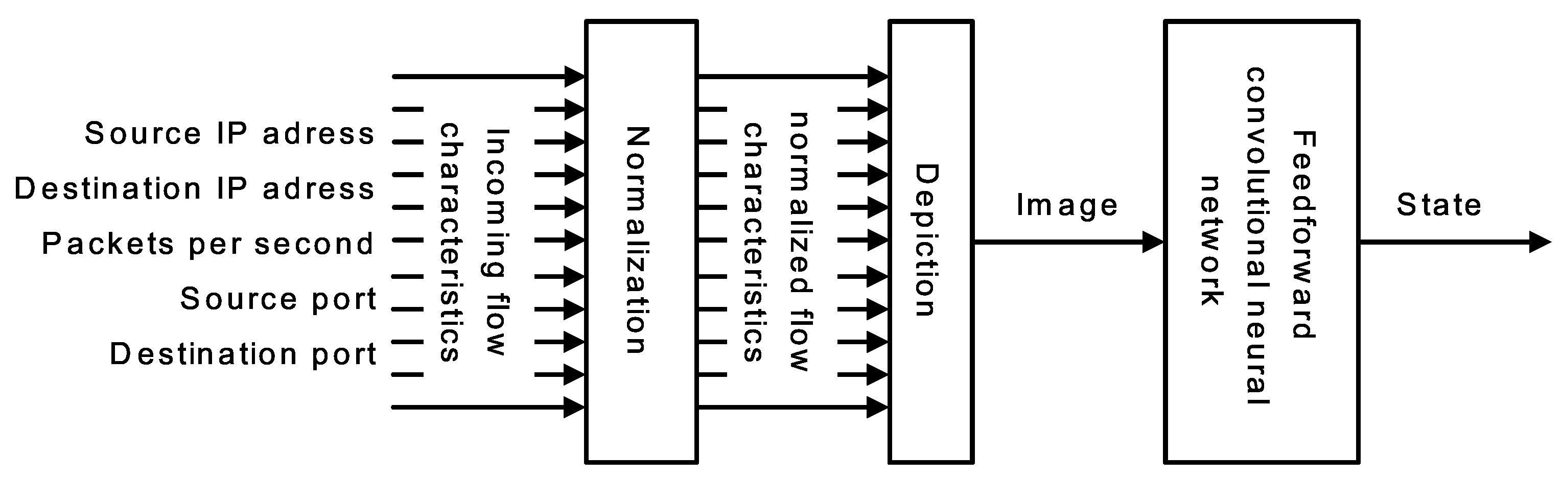
Section 1.3, the programmability of SDN allows us to extend the SDN controller with an AI-based protection functionality. One of the obvious applications of AI is the advanced traffic handling, and consequently, automated filtering during an SDN-based firewall’s operation. The AI element functionality is often supposed to work as a decision element. In most cases, the AI element helps to determine one of the decision states according to incoming flow characteristics.
In this article, we introduce a specific neural network-based decision procedure that can be considered for application in any flow characteristic-based traffic handling controller. For the sake of being concise and transparent, we consider the decision element state space to be composed of the following items: allow, block, forward to selected ports, application layer inspection and four levels of quality of service (QoS) settings (low, normal, high and critical). For the same reason, we consider only L4 communication, as described in
Section 3.2.1. Nevertheless, the decision element, which includes other possible communication protocols and an extended set of items in the state space, can be developed using the same procedure.
Therefore, in order to demonstrate the idea of this contribution, we aim to develop a decision procedure capable of making a decision based upon the incoming flow characteristics defined by both source and destination IPv4 addresses and also by the amount of traffic expressed as packets per second. Each IP address is composed of four octets, which are used as unique inputs. In addition, source and destination port numbers are considered as relevant inputs. Hence, 11 inputs specify the decision.
While regarding artificial neural network as an engine for the decision procedure, we will describe briefly below three hypotheses to develop the traffic handling controller described above.
2.1. Feedforward Neural Network Applied Directly to Map Input–Output Dependency
During the past three decades, feedforward multilayer neural networks with dense layers have proven themselves to be specifically competent for input–output mapping problems. If a feedforward neural network meets specific conditions [
20,
21], it is able to solve any input–output problem to any degree of accuracy. Hence, in this case, a feedforward neural network is supposed to determine the decision state from the incoming flow characteristic as shown in
Figure 1.
This hypothesis is closely dealt with in the authors’ previous works [
9,
22] and is used here for the purpose of comparing the results.
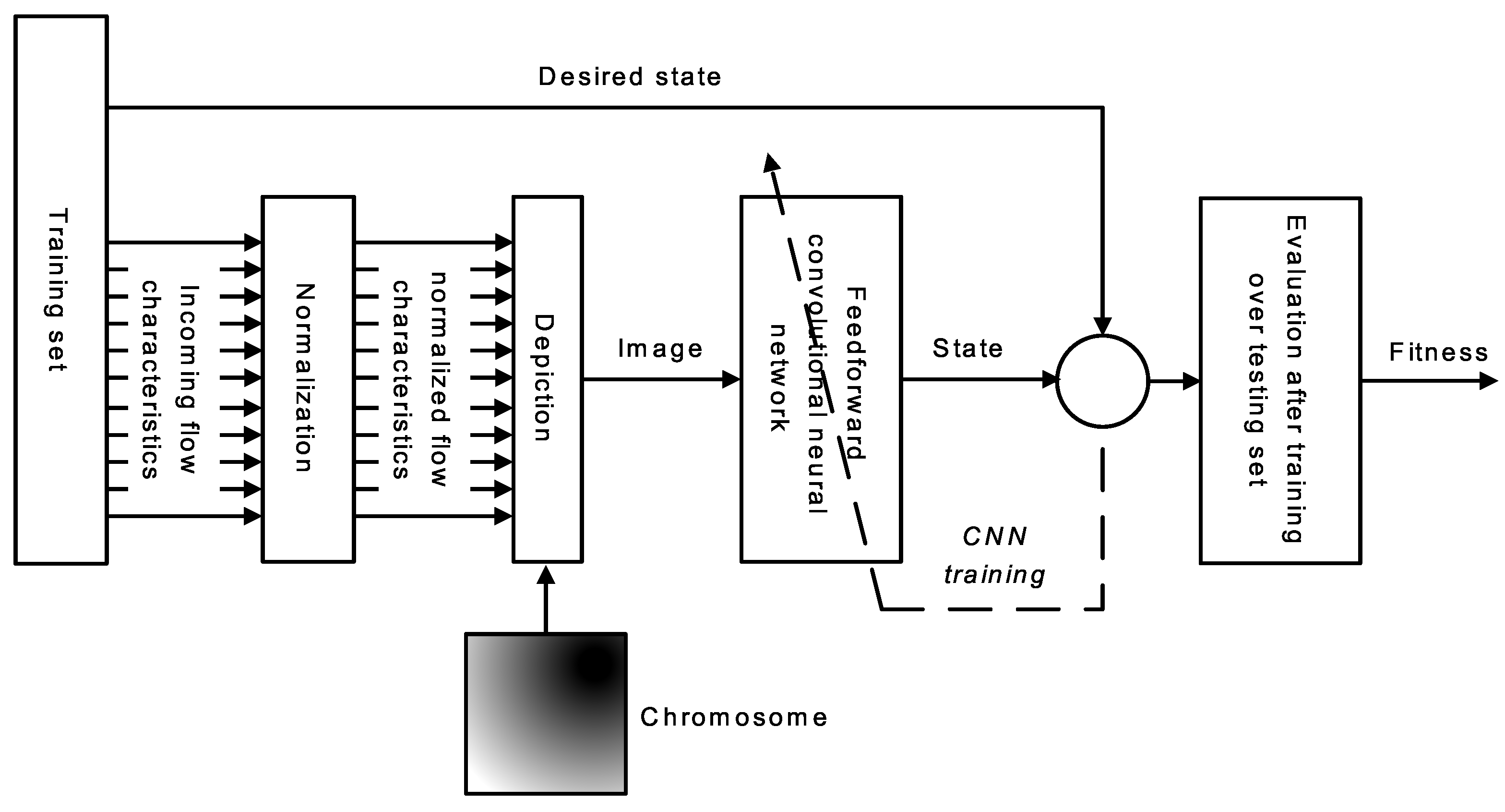
2.2. A Convolutional Neural Network and Depiction Applied to Map Input–Output Dependency
With current possibilities in hardware acceleration of parallel computing, convolutional neural networks (CNNs) are considered to constitute a leading topology among neural networks. In addition to dense layers of classical feedforward neural networks, CNNs include a convolutional layer that extracts features from the input signal. A good summary of CNNs can be found in [
23]. A list of well-known CNN topologies is summarized in [
24]. Therefore, in this case, a convolutional neural network is expected to determine the decision state from the incoming flow characteristic, as demonstrated in
Figure 2.
It is a generally accepted feature of CNNs that the performance is particularly efficient when applied to multidimensional data processing. Image processing can be mentioned as one of the most recognizable such examples [
25]. Hence, it seems to be efficient to find an operation that transforms 11 inputs (incoming flow characteristics) into a two- or three-dimensional structure, preferably a graphical figure. This operation is further referred to as depiction. A polar line chart is one of the suggested transformations, as demonstrated in
Figure 3.
This hypothesis, and the previous one, is analyzed in the authors’ earlier work [
22] and is used here for the purpose of comparing the results.
2.3. Convolutional Neural Network with Optimized Depiction Procedure Applied to Map Input-Output Dependency
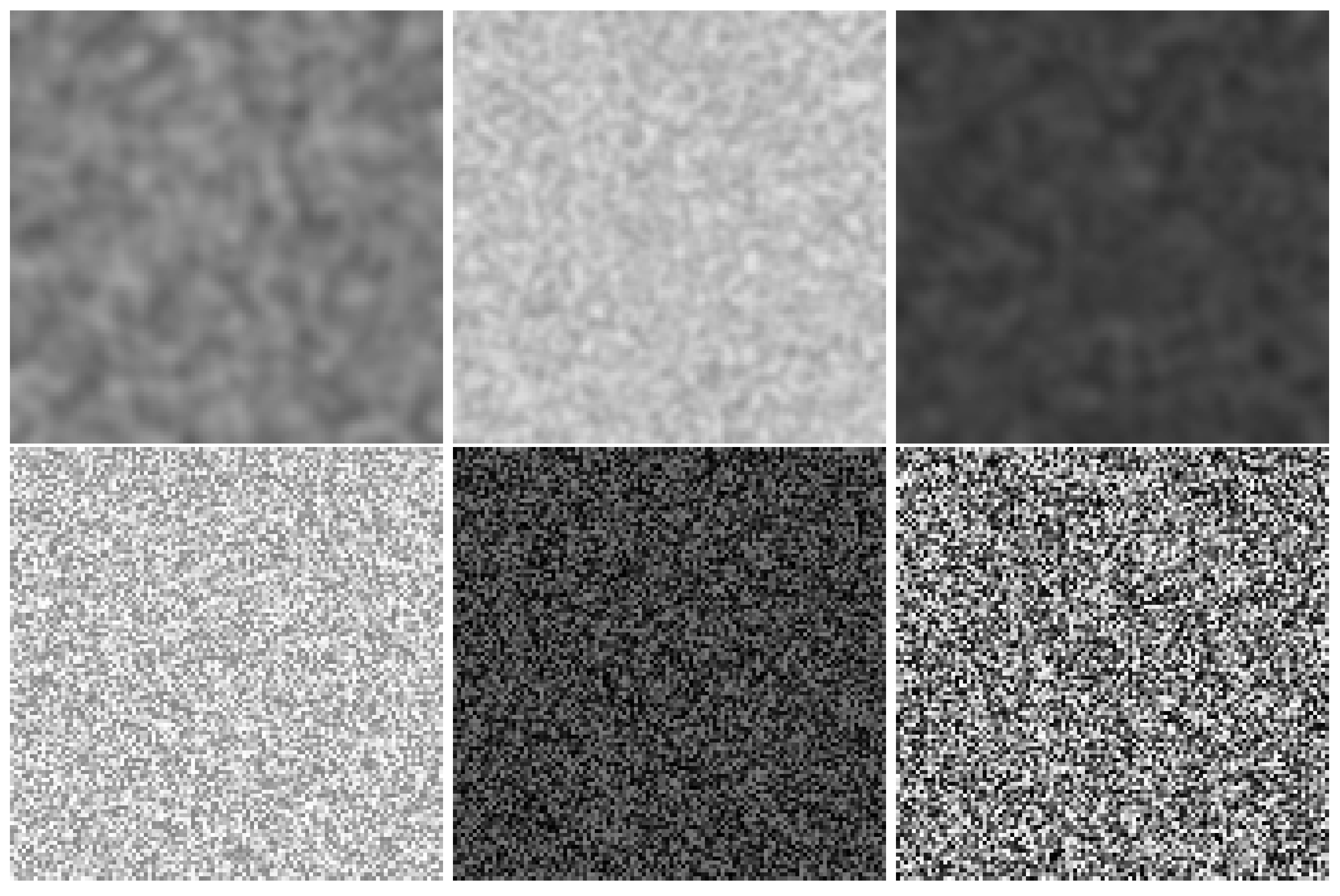
This hypothesis is an expansion of the previous one and is the point of this contribution. We expect that the depiction procedure stated above strongly affects the accuracy of the decision determination. Therefore, it should be optimized in order to provide an ideal medium that supplies incoming flow characteristics to the CNN. In this contribution, we propose an approach for depiction procedure optimization as shown in
Figure 4. The approach involves repeated CNN training utilizing the data obtained by various depiction procedures. The procedure itself, meanwhile, is tuned according to the performance of the trained CNN.
This hypothesis is defined in detail in the following section. The testing experiments are then presented, and the results are then compared to those from other approaches at the end of the article.
2.4. Depiction Procedure Optimization
The key step of this contribution is to determine the optimal procedure for depiction. In our case, the process of depiction was supposed to transform 11 values of incoming flow characteristics into a 2D array suitable for processing by the CNN. In addition, the process was meant be quick enough to be used in SDN. Therefore, after pilot testing of several approaches, we decided to apply a depiction procedure based on planar rotation of annuli of the original medium image, since this geometric transformation can be implemented in a very efficient way. To be specific, the medium image was divided into homocentric annuli. The number of annuli equaled the number of parameters. Then, each annulus was rotated depending on the value of the corresponding parameter. An example of four parameters is depicted in
Figure 5.
The quality of depiction is strongly affected, however, by the entity of the medium image. In other words, a correctly defined medium image will provide a much more readable input to the CNN than will a random medium image. On the other hand, the “correctness” of the medium image is not directly observable and must be determined by evaluating the performance of the whole decision element. Hence, the medium image pattern is the subject of optimization.
As the image pattern, which affects the CNN, should be the result of the optimization process, it would be difficult to adapt classical techniques from mathematical optimization to provide the optimal solution. On the other hand, the family of stochastic population-based optimization techniques (evolutionary algorithms) seems to be a perfect fit, because these techniques do not demand derivative evaluation or a gradient of objective function. To justify this selection, in the following paragraphs, we briefly review evolutionary algorithms applied in cybersecurity.
2.5. Work Related to Applications of Evolutionary Algorithms in Cybersecurity
Evolutionary algorithms, together with other soft computing techniques, have proven themselves to have great potential in the cybersecurity field. Even articles older than 10 years describe evolutionary algorithms to provide successful and efficient tools, especially in detecting intrusion [
26,
27,
28]. In these works, evolutionary algorithms were used for deriving classification rules. In other cases, evolutionary algorithms were used instead to select optimal parameters of some core functions within which other methods were used to derive the rules [
29].
In more recent works, there has been a focus especially on (D)DoS protection systems developed using evolutionary algorithms and other artificial intelligence techniques. The advantage of these systems lies in their ability to learn from current data. Hence, these systems are able to prevent attacks even if the attackers implement different traffic patterns [
30,
31].
A different domain is addressed in [
32,
33]. Dennis Garcia et al. provide a cybersecurity project for developing network defense strategies through modeling adversarial network attack and defense dynamics in peer-to-peer networks via coevolutionary algorithms.
Apart from the mentioned usages, evolutionary algorithms are used in addressing many of today’s most recent issues within networking, such as routing, quality of service, load balancing, bandwidth allocation and channel assignment [
34,
35].
2.6. Genetic Algorithm for Medium Image Pattern
A genetic algorithm (GA) is probably the most commonly encountered member of the evolutionary algorithms family. It is a stochastic search method for finding a near optimum solution based on a natural selection process and genetics [
36]. The GA uses a population of chromosomes representing possible solutions to the problem. In each generation, the GA creates a new set of possible solutions by selecting chromosomes according to their level of fitness. The selected chromosomes are then bred together using genetic operators, mainly crossover and mutation. This iterative process is expected to lead to better solutions.
The particular parts of the GA, and how we implement them to solve our problem, are summarized below. Note that each step depends on many tunable parameters. As it would be impossible to set each of them analytically, most of them are selected based on limited pilot studies performed during the experiments.
2.6.1. Solution Representation
As mentioned above, each chromosome represents a possible solution to the problem. We want to determine an optimal pattern of a medium image for the depiction procedure. Hence, the chromosome is represented by a 2D square array with 110 rows and columns. We believe that this size is a compromise reached by considering computational complexity and gains in accuracy. In addition, this size can be processed by all the selected CNNs (see
Section 3.2). Each cell in a 2D array is filled by a value in the range
. Therefore, this array can be visualized as an 8 bit grayscale image.
2.6.2. Fitness Evaluation
Each chromosome in the population needs to be evaluated by its fitness level in order to perform selection. In our case, the chromosome represents a medium image for depiction procedure. This procedure affects the input into the CNN, and consequently, the performance of the CNN. Therefore, each individual was evaluated by the performance of the CNN trained using our dataset (see
Section 3.2.1), transformed using a specific depiction procedure. The process of evaluation is shown in
Figure 6. The final fitness was evaluated as the mean value of the best performances of each particular CNN. The performance is defined as a categorical cross entropy loss function.
Apparently, the fitness evaluation procedure is a very stochastic process, especially due to the CNN’s training. Therefore, we decided to train three well-established CNNs in one evaluation. Each CNN was trained five times. Hence, 15 training processes were performed during one fitness level evaluation. We expected this to be sufficient for suppressing the stochasticity of the procedure. As CNNs, we selected LeNet-5 [
37,
38], AlexNet [
39] and VGG-16 net [
40]. Note that because the fitness level is based on some kind of loss function, lower fitness means a better chromosome.
All the parameters are summarized in
Table 1.
2.6.3. Initialization
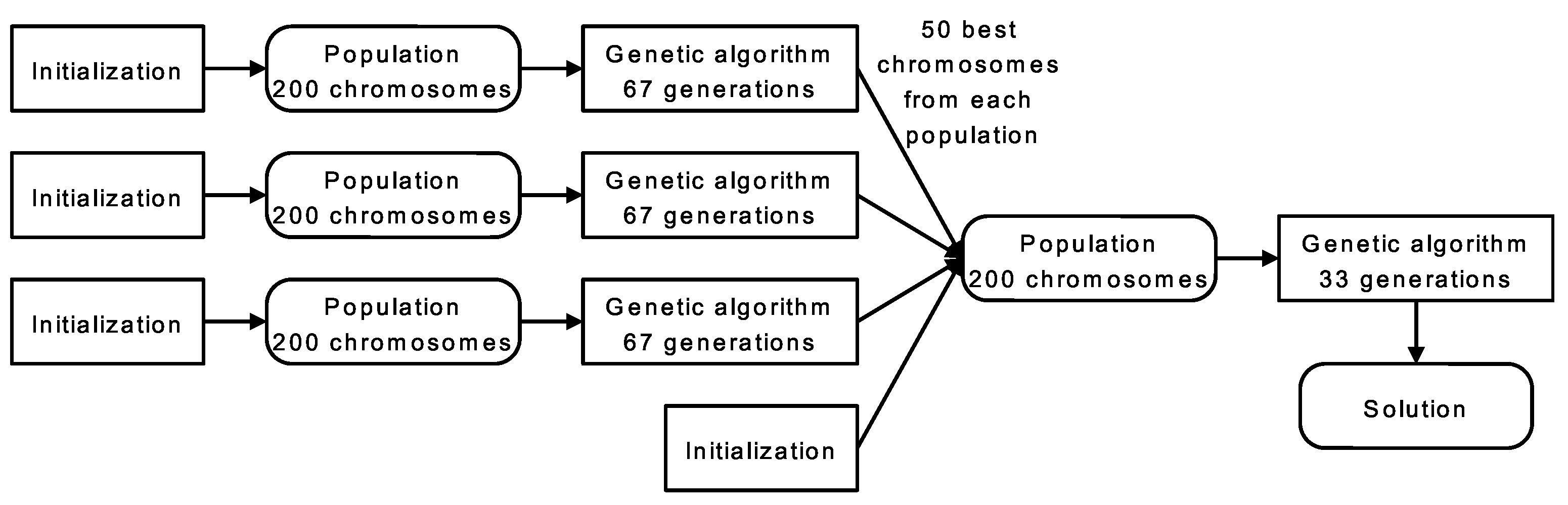
Population initialization is the starting point of the GA. During initialization, all chromosomes in the initial population are set. We select the heuristic initialization method as follows:
20% of chromosomes set as an array of random integer in range ;
20% of chromosomes set as an array of random integer in range ;
20% of chromosomes set as an array of random integer in range ;
20% of chromosomes set as an array of random integer in range ;
20% of chromosomes set as an array of random integer in range .
Each chromosome is then filtered by Gaussian filter, where the standard deviation is set randomly in range .
Some examples of initial chromosomes are shown in
Figure 7.
2.6.4. Selection
Selection is that step of the GA where individual chromosomes are selected from a population for breeding. We choose to use tournament selection. To be more specific, n tournaments are arranged, where n is the number of chromosomes within a population. Four chromosomes randomly selected from the population participate in each tournament. Eventually, the winner of each of n tournaments is selected for breeding.
2.6.5. Crossover
Crossover is a genetic operator used to combine the genetic code of two or more parent chromosomes to provide new (offspring) chromosomes. Crossover provides stochasticity to the process by creating completely new chromosomes. In our case, where the chromosomes are represented by grayscale images, the process of crossover is defined as follows:
Get two parent chromosomes a and b from population;
set to a random value in range ;
limit to a range ;
set number of crossover points to integer in range ;
for each crossover point:
- –
divide both parents a and b along the crossover point into rectangles and respectively ;
- –
set for ;
- –
set for ;
- –
set a as composition of ;
- –
set b as composition of ;
return a, b as the result of crossover.
Note that there is the same probability for to be at its limits or between them.
For better illustration of the crossover operation, some examples of crossovers are shown in
Figure 8,
Figure 9 and
Figure 10.
2.6.6. Mutation
Mutation is an operation in the GA to maintain genetic diversity within the population. Selection and crossover naturally reduce diversity of chromosomes, and this could lead the algorithm into an unwanted local optimum. Hence, mutation is an essential operator to keep the diversity sufficiently high.
We implement two types of mutation, each performed on every chromosome with probability 0.025. Both types of mutation are described below.
Define a square subarray from a chromosome with random position and random size (maximum number of rows and columns is 40). Create a subarray of the same size by the initialization procedure defined in
Section 2.6.3. Place the created subarray into the position of the original subarray.
Filter the chromosome using the Gaussian filter, where standard deviation is set randomly in the range .
Two examples of the mutation procedure are depicted in
Figure 11.
2.6.7. Elitism
Elitism in the GA is a procedure allowing the best chromosomes from the current generation to migrate unaltered directly to the next generation. Elitism generally guarantees that the solution quality of the best chromosome will not decrease over generations. In our implementation, we simply migrated the best solution (one chromosome) from its current population to the next generation. Note that the best chromosome still can be selected for crossover and mutation, even if selected for elitism.
2.6.8. Optimization Flow
Considering the statements above, we design the optimization procedure in order to obtain the ideal medium image for the depiction procedure. Note that all the steps, especially fitness function evaluation, are computationally demanding, so we implemented several heuristics to improve the probability of being successful. Specifically, we designed the experiment as follows.
First, we initiated three encapsulated populations of 200 individual chromosomes. Each population was evolved for 67 generations. Then, the 50 best chromosomes from each encapsulated population, together with 50 freshly initiated chromosomes, were put together to create a new population. This new population was evolved for the next 33 generations. The optimization procedure is shown in
Figure 12.
3. Results
In this section, we provide the process and results of the depiction procedure optimization, and afterwards, results of the whole decision procedure design.
3.1. Depiction Procedure Design
We performed the optimization experiment according to the statements summarized in the previous section. In
Figure 13, a course of the fitness level is shown for a mean chromosome and for the best chromosome from all populations. Several interesting points are worthy of note. Through the first 67 generations, the fitness of the best individual steadily declines. Then, after integration of all the populations, the fitness of the best chromosome falls steeply for several generations before eventually becoming constant. This course indicates that the optimization process is set suitably and the number of generations is sufficiently high. If we examine the course of the mean chromosome, we can observe that the mutation operator ensures a sufficiently high diversity in the population for the first 67 populations. The diversity then ascends, obviously because of freshly initiated chromosomes. The diversity in the last 20–25 generations is conspicuously lower (note the logarithmic scale on the y-axis). In addition, the stochastic process of neural network training is still observable on both courses.
It is obvious that this optimization experiment could be run repeatedly for different parameters. However, as mentioned above, it is computationally a very demanding task. This one experiment ran for more than four months using three computers having hardware-accelerated parallel processing. To be more specific, we used computers with the following hardware specifications: processor—Intel Core i5-8600K (3.6 GHz); internal memory—16 GB DDR4 (2666 MHz); video card—NVIDIA PNY Quadro P5000 16 GB GDDR5x PCIe 3.0 (2560 CUDA cores); SSD—SATA M.2 512 GB. The experiments were performed using Python 3.6 and TensorFlow 2.0.
The chromosome with the best fitness level at the end of the optimization process is shown in
Figure 14. This pattern is used as the medium image for the depiction procedure.
3.2. Decision Procedure Design
In this section, we aim to develop a CNN-based decision element for a decision procedure according to
Figure 2. This process is especially based on training and testing of the implemented CNN. Feedforward CNNs consist of multiple layers arranged in a feed-forward manner. The first layers (convolutional and max-pooling, typically combined with ReLU) perform feature extraction from the input data. Then, several dense layers are connected and the classification or decision is ensured by a soft-max activation function.
As the performance of the CNN is strongly affected by its structure, we decided to include several well-known architectures for testing. Namely, Net1 and Net2 are the simplest architectures. Both of these were adapted from [
41]. In addition to these networks, the following more complex and widely accepted topologies were selected: LeNet-5 [
37,
38], AlexNet [
39], VGG-16 net [
40] and MobileNet [
42]. Note that more advanced CNNs were not included into this selection because of the strong need for computational efficiency. More recent CNNs are generally much more computationally demanding.
3.2.1. Training Dataset
The dataset used simulates a highly utilized industrial network corresponding to an electrical substation network [
43] with control and management applications such as SCADA and Distribution Management System. In order to make the solution reasonably coherent, lower-layer industrial protocols such as GOOSE were not considered. The traffic was generated by a custom developed application [
9], which in turn generated the target decisions (ALLOW, BLOCK, INSPECTION, FORWARD, QOS EF, QOS AF13, and QOS AF41). Data traffic was generated for the following scenarios: normal traffic (random TCP or UDP ports and action: ALLOW), DoS attack (number of packets per second for a single flow distinctly high and action: BLOCK), HTTP traffic (TCP destination port 80 and action: application layer INSPECTION), HTTPS traffic (TCP destination port 443 and action: FORWARD to selected ports) and three types of QoS (critical priority for TCP destination port 5060; high priority for TCP destination port 37; and low priority for source or destination ports 20, 21, 69 and 115). IP addresses and number of packets per second were randomly generated from defined intervals. The traffic map generated for neural network training consisted of 80,000 unique data patterns.
The dataset was subdivided into a training set (70%), validation set (15%) and testing set (15%). The training set was used for neural network parameter adaptation during the training process, the validation set was used to identify the best network configuration during training and the testing set was used for final AI module evaluation.
Note that inputs in the dataset were transformed using the depiction procedure described in
Figure 5 and using the medium image shown in
Figure 14.
3.2.2. CNN Training and Results
The training of the selected architectures was performed in order to obtain a CNN-based decision element. The ADAM search technique was chosen for use as an optimizer based on its generally acceptable performance [
44]. Initial weights were set randomly, with Gaussian distribution (location = 0, scale = 0.05). The training instances were performed 50 times. See
Table 2 for all parameters of the training processes. The resulting values of the categorical cross entropy loss function computed over the testing set for each topology are shown in
Figure 15. Categorical cross entropy loss function is calculated as follows.
where
N is the number of samples in the testing set,
K is the number of classes considered for classification,
t is the label of the target class (0 or 1) and
y is the
-th scalar value in the neural network output (between 0 and 1).
In addition, accuracy of the decision element when using the data in the testing set is depicted in
Figure 16. As training is a stochastic process, the results are depicted as box graphs. Accuracy is defined as follows.
where
n is the number of correctly performed decisions and
N is the number of all decisions, i.e., the number of samples in the testing set.
As mentioned in
Section 2, we have tested three hypotheses in our research. The best final accuracies of the decision element designed in this contribution are compared to our previous results in
Table 3. In addition, we include other important metrics—confusion matrix, precision, recall and F1-score—in
Appendix A.
4. Discussion
The objective of the presented work was to develop a specific neural network-based decision procedure that may be applied to a flow characteristic-based traffic handling controller. Three hypotheses were formulated and tested in this and the authors’ previous works. It already has been shown that the convolutional neural network in combination with a depiction procedure provides better accuracy of the decision element in comparison to a direct feedforward neural network [
22]. We clearly show in this contribution, however, that it is beneficial to optimize the depiction procedure itself. As the results demonstrate (
Table 3), optimization of the depiction procedure improves the accuracy from 0.9501 to 0.9984 while preserving the same computational complexity. In addition, the other metrics presented in
Appendix A also support this statement. For example, according to
Table A11, (D)DoS attack was correctly detected in 6204 cases of 6218 possible cases and no false detections were triggered.
Although the optimization process is a hugely time-consuming task, it was performed once during the development of the decision procedure and it did not affect implementation of the element in traffic handling control.
The proposed AI decision procedure can be generally utilized in many network security devices such as firewalls, intrusion detection systems and intrusion prevention systems. In our protection system deployment, as formerly introduced in [
9], the functionality combines intrusion prevention and detection systems. Use of SDN relies on periodical collection of traffic data (commonly every one second interval) and subsequent processing on the SDN controller, which includes the AI subsystem. This processing is therefore done offline as in traditional intrusion detection systems. However, unlike in these systems, our system can react based on the AI subsystem result, by inserting specific flow rules (such as blocking) into networking devices and therefore achieving functionality of the intrusion prevention system, but with an approximately 1 s latency. For testing purposes, we deploy the proposed decision procedure using NVIDIA Jetson NANO [
45], as a single board computer naturally suitable for this purpose. The latency of the depiction procedure is 18.6 ms and the latency of the MobileNet (which provides the best overall performance—see below) is 16.6 ms. We assume, the decision procedure could take from approximately 2 ms to 100 ms, based on used hardware and neural network architecture. Therefore, it can be seamlessly applied in the SDN-based network protection system with a one second interval.
In examining performance of the particular convolutional networks, we should emphasize especially the well-established VGG-16 and MobileNet, which feature good learning ability, result in small loss function values and deliver excellent performance with accuracies equal to 0.9976 and 0.9984, respectively. Surprisingly, LeNet-5’s accuracy fails to exceed 0.95.
It is not possible to directly compare the presented results to other works. Although several authors propose artificial intelligence techniques for security handling, using the software-defined networking paradigm, they mostly consider different aims, unmatched datasets and uneven conditions. For a raw illustration, we summarize some findings below.
Authors in [
46] proposed an intrusion detection system for SDN based on a neural network approach and they achieved the accuracy of 0.973 with their dataset. Oo Myo Myint et al. [
47] introduced a detection method of (D)DoS attack by using the advanced support vector machine technique with an accuracy between 0.970 and 1.000 based on the ratio of training and testing data. They also used their own dataset. Fuzzy logic approaches can also be used for detection of the (D)DoS attack on SDN. Authors [
48] proposed an algorithm that deployed multiple criterion for attack detection, and they demonstrated the ability to detect and filter 97% of the attack flows with a false positive rate of 5%. Moreover, a combination of a support vector machine and a decision tree approach was introduced in [
49]. Based on the experimental results with the KDD CUP99 dataset [
50], their system showed an accuracy of 0.976. Additionally, as a last example, Phan et al. [
51] provided a novel approach which implemented a self-organizing map with a support vector machine approach. Their results showed that this system was able to achieve an accuracy of 0.976 and a false positive rate of 3.85%. As mentioned, these results were gained from different datasets and the acquisition procedures were based on different effects. Despite this, the presented accuracies are roughly on the same level as our results, or worse. These findings indicate that our approach is vindicated.
5. Conclusions
In this contribution, we proposed a specific neural network-based decision procedure as a part of a traffic handling controller. Such an AI-based element can be straightforwardly integrated into a software-defined networking controller to provide all the advantages of a machine learning approach while presenting no particular demands for proprietary software or custom hardware.
The main contribution consists of the development and improvement of the depiction process using a genetic algorithm. We implemented a convolutional neural network as a decision element. In as much as convolutional neural networks behave especially well when applied to multidimensional inputs, we state a novel depiction procedure to automatically transform incoming flow characteristics into a 2D array. The depiction procedure uses meta-learning to adaptively perform an efficient conversion of raw data into a new data representation (suitable encoder), which will be suitable for processing using a convolutional neural network. The depiction procedure adds another layer of representational learning (one layer of representational learning is contained in a deep neural network) and is optimized in a complex computational experiment based on a genetic algorithm.
As a result, we demonstrated that a convolutional network, in combination with an optimized depiction procedure, provides exceptionally high accuracy of the decision process. The proposed process of finding a suitable data representation and an effective depiction procedure on the performed experiments, significantly increases the accuracy in the classification of network packets. The presented method is, nevertheless, far from optimal. One important point is the size and bit depth of the medium image—these parameters are now determined once without the possibility of a change. It could be possible to find the size and depth more suitable for a particular neural network. The other point is the depiction process. Many well accepted approaches, which can store information into an image, are known. Instead of using our procedure, we can adapt other one and get a better or less time-consuming depiction process.
Moreover, we believe that the proposed depiction procedure could be used much more generally, and that it could be applicable to other problems that do not yet have good enough results when using neural networks. Future research will focus on designing and exploring different types of depiction procedures and finding more general approaches that could increase the accuracy of neural networks and machine learning algorithms on selected problems.
Author Contributions
Conceptualization, P.D. and F.H.; methodology, P.D. and J.M.; software, P.D. and F.H.; validation, P.D., F.H. and D.S.; formal analysis, P.D.; investigation, P.D.; resources, F.H.; writing—original draft preparation, P.D.; writing—review and editing, P.D. and F.H.; visualization, P.D.; supervision, P.D.; project administration, P.D.; funding acquisition, P.D. All authors have read and agreed to the published version of the manuscript.
Funding
The work has been supported from the supported from the programme INTER-EXCELLENCE (LTAIN19100) funds of the Ministry of Education, Youth and Sports, Czech Republic, project LTAIN19100 “Artificial Intelligence Enabled Smart Contactless Technology Development for Smart Fencing”. This support is very gratefully acknowledged.
Institutional Review Board Statement
Not applicable.
Informed Consent Statement
Not applicable.
Data Availability Statement
Conflicts of Interest
The authors declare no conflict of interest.
Abbreviations
The following abbreviations are used in this manuscript:
| AI | Artificial Intelligence |
| CNN | Convolutional Neural Network |
| (D)DoS | Distributed Denial of Service |
| GA | Genetic Algorithm |
| IoT | Internet of Things |
| NFV | Network Function Virtualisation |
| QoS | Quality of Service |
| SDN | Software Defined Networking |
Appendix A. Metrics of Designed Neural Networks
We present the accuracy of each neural network intended to be a decision element in
Table 3. However, in order to provide a comprehensive information about the process, we provide the other metrics here as an appendix. In the following tables, we present a confusion matrix, precision, recall and F1-scorescore for the best representative of each neural network and each class. The metrics are defined as follows.
where TP (true positive) is the number of correctly recognized decisions for each class (ALLOW, BLOC, INSPECTION, …), FP (false positive) is is the number of incorrectly recognized decisions for a specific class and FN (false negative) is the number of decisions wherein the specific class was not recognized.
Table A1.
Confusion matrix for Net1.
Table A1.
Confusion matrix for Net1.
| | Allow Predicted | Block Predicted | Forward Predicted | Inspection Predicted | QoS_af13 Predicted | QoS_af41 Predicted | QoS_ef Predicted |
|---|
| Allow Actual | 3164 | 0 | 16 | 3 | 21 | 1 | 24 |
| Block Actual | 31 | 6187 | 0 | 0 | 0 | 0 | 0 |
| Forward Actual | 0 | 0 | 3133 | 0 | 1 | 0 | 0 |
| Inspection Actual | 0 | 0 | 0 | 3062 | 14 | 0 | 0 |
| QoS af13 Actual | 2 | 0 | 2 | 425 | 2059 | 634 | 2 |
| QoS af41 Actual | 0 | 0 | 0 | 0 | 15 | 3119 | 0 |
| QoS ef Actual | 0 | 0 | 0 | 0 | 1 | 0 | 3084 |
Table A2.
Classification report for Net1.
Table A2.
Classification report for Net1.
| | Precision | Recall | F1-Score | Samples |
|---|
| Allow | 0.9897 | 0.9799 | 0.9847 | 3229 |
| Block | 1.0000 | 0.9950 | 0.9975 | 6218 |
| Forward | 0.9943 | 0.9997 | 0.9970 | 3134 |
| Inspection | 0.8774 | 0.9954 | 0.9327 | 3076 |
| QoS af13 | 0.9754 | 0.6591 | 0.7866 | 3124 |
| QoS af41 | 0.8308 | 0.9952 | 0.9056 | 3134 |
| QoS ef | 0.9916 | 0.9997 | 0.9956 | 3085 |
Table A3.
Confusion matrix for Net2.
Table A3.
Confusion matrix for Net2.
| | Allow Predicted | Block Predicted | Forward Predicted | Inspection Predicted | QoS_af13 Predicted | QoS_af41 Predicted | QoS_ef Predicted |
|---|
| Allow Actual | 3161 | 0 | 17 | 4 | 17 | 3 | 27 |
| Block Actual | 28 | 6190 | 0 | 0 | 0 | 0 | 0 |
| Forward Actual | 0 | 0 | 3133 | 0 | 1 | 0 | 0 |
| Inspection Actual | 0 | 0 | 0 | 3072 | 4 | 0 | 0 |
| QoS af13 Actual | 1 | 0 | 3 | 571 | 1816 | 730 | 3 |
| QoS af41 Actual | 0 | 0 | 0 | 0 | 11 | 3123 | 0 |
| QoS ef Actual | 0 | 0 | 0 | 0 | 1 | 0 | 3084 |
Table A4.
Classification report for Net2.
Table A4.
Classification report for Net2.
| | Precision | Recall | F1-Score | Samples |
|---|
| Allow | 0.9909 | 0.9789 | 0.9849 | 3229 |
| Block | 1.0000 | 0.9955 | 0.9977 | 6218 |
| Forward | 0.9937 | 0.9997 | 0.9967 | 3134 |
| Inspection | 0.8423 | 0.9987 | 0.9139 | 3076 |
| QoS af13 | 0.9816 | 0.5813 | 0.7302 | 3124 |
| QoS af41 | 0.8099 | 0.9965 | 0.8936 | 3134 |
| QoS ef | 0.9904 | 0.9997 | 0.9950 | 3085 |
Table A5.
Confusion matrix for LeNet-5.
Table A5.
Confusion matrix for LeNet-5.
| | Allow Predicted | Block Predicted | Forward Predicted | Inspection Predicted | QoS_af13 Predicted | QoS_af41 Predicted | QoS_ef Predicted |
|---|
| Allow Actual | 3167 | 1 | 17 | 4 | 21 | 1 | 18 |
| Block Actual | 38 | 6179 | 0 | 0 | 0 | 1 | 0 |
| Forward Actual | 0 | 0 | 3130 | 0 | 4 | 0 | 0 |
| Inspection Actual | 0 | 0 | 0 | 2949 | 127 | 0 | 0 |
| QoS af13 Actual | 3 | 0 | 2 | 545 | 2068 | 504 | 2 |
| QoS af41 Actual | 0 | 0 | 0 | 0 | 128 | 3006 | 0 |
| QoS ef Actual | 0 | 0 | 0 | 0 | 2 | 0 | 3083 |
Table A6.
Classification report for LeNet-5.
Table A6.
Classification report for LeNet-5.
| | Precision | Recall | F1-Score | Samples |
|---|
| Allow | 0.9872 | 0.9808 | 0.9840 | 3229 |
| Block | 0.9998 | 0.9937 | 0.9968 | 6218 |
| Forward | 0.9940 | 0.9987 | 0.9963 | 3134 |
| Inspection | 0.8431 | 0.9587 | 0.8972 | 3076 |
| QoS af13 | 0.8800 | 0.6620 | 0.7556 | 3124 |
| QoS af41 | 0.8559 | 0.9592 | 0.9046 | 3134 |
| QoS ef | 0.9936 | 0.9994 | 0.9964 | 3085 |
Table A7.
Confusion matrix for AlexNet.
Table A7.
Confusion matrix for AlexNet.
| | Allow Predicted | Block Predicted | Forward Predicted | Inspection Predicted | QoS_af13 Predicted | QoS_af41 Predicted | QoS_ef Predicted |
|---|
| Allow Actual | 3185 | 0 | 11 | 0 | 24 | 0 | 9 |
| Block Actual | 33 | 6185 | 0 | 0 | 0 | 0 | 0 |
| Forward Actual | 0 | 0 | 3134 | 0 | 0 | 0 | 0 |
| Inspection Actual | 0 | 0 | 0 | 3076 | 0 | 0 | 0 |
| QoS af13 Actual | 1 | 0 | 2 | 0 | 3120 | 0 | 1 |
| QoS af41 Actual | 0 | 0 | 0 | 0 | 5 | 3129 | 0 |
| QoS ef Actual | 2 | 0 | 0 | 0 | 0 | 0 | 3083 |
Table A8.
Classification report for AlexNet.
Table A8.
Classification report for AlexNet.
| | Precision | Recall | F1-Score | Samples |
|---|
| Allow | 0.9888 | 0.9864 | 0.9876 | 3229 |
| Block | 1.0000 | 0.9947 | 0.9973 | 6218 |
| Forward | 0.9959 | 1.0000 | 0.9979 | 3134 |
| Inspection | 1.0000 | 1.0000 | 1.0000 | 3076 |
| QoS af13 | 0.9908 | 0.9987 | 0.9947 | 3124 |
| QoS af41 | 1.0000 | 0.9984 | 0.9992 | 3134 |
| QoS ef | 0.9968 | 0.9994 | 0.9981 | 3085 |
Table A9.
Confusion matrix for VGG-16.
Table A9.
Confusion matrix for VGG-16.
| | Allow Predicted | Block Predicted | Forward Predicted | Inspection Predicted | QoS_af13 Predicted | QoS_af41 Predicted | QoS_ef Predicted |
|---|
| Allow Actual | 3186 | 4 | 11 | 0 | 21 | 0 | 7 |
| Block Actual | 18 | 6200 | 0 | 0 | 0 | 0 | 0 |
| Forward Actual | 0 | 0 | 3134 | 0 | 0 | 0 | 0 |
| Inspection Actual | 0 | 0 | 0 | 3076 | 0 | 0 | 0 |
| QoS af13 Actual | 2 | 0 | 3 | 10 | 3107 | 1 | 1 |
| QoS af41 Actual | 0 | 0 | 0 | 0 | 0 | 3134 | 0 |
| QoS ef Actual | 1 | 0 | 0 | 0 | 3 | 0 | 3081 |
Table A10.
Classification report for VGG-16.
Table A10.
Classification report for VGG-16.
| | Precision | Recall | F1-Score | Samples |
|---|
| Allow | 0.9935 | 0.9867 | 0.9901 | 3229 |
| Block | 0.9994 | 0.9971 | 0.9982 | 6218 |
| Forward | 0.9956 | 1.0000 | 0.9978 | 3134 |
| Inspection | 0.9968 | 1.0000 | 0.9984 | 3076 |
| QoS af13 | 0.9923 | 0.9946 | 0.9934 | 3124 |
| QoS af41 | 0.9997 | 1.0000 | 0.9998 | 3134 |
| QoS ef | 0.9974 | 0.9987 | 0.9981 | 3085 |
Table A11.
Confusion matrix for MobileNet.
Table A11.
Confusion matrix for MobileNet.
| | Allow Predicted | Block Predicted | Forward Predicted | Inspection Predicted | QoS_af13 Predicted | QoS_af41 Predicted | QoS_ef Predicted |
|---|
| Allow Actual | 3193 | 0 | 10 | 0 | 20 | 0 | 6 |
| Block Actual | 14 | 6204 | 0 | 0 | 0 | 0 | 0 |
| Forward Actual | 0 | 0 | 3134 | 0 | 0 | 0 | 0 |
| Inspection Actual | 0 | 0 | 0 | 3076 | 0 | 0 | 0 |
| QoS af13 Actual | 2 | 0 | 3 | 0 | 3114 | 1 | 4 |
| QoS af41 Actual | 0 | 0 | 0 | 0 | 0 | 3134 | 0 |
| QoS ef Actual | 0 | 0 | 0 | 0 | 0 | 0 | 3085 |
Table A12.
Classification report for MobileNet.
Table A12.
Classification report for MobileNet.
| | Precision | Recall | F1-Score | Samples |
|---|
| Allow | 0.9950 | 0.9889 | 0.9919 | 3229 |
| Block | 1.0000 | 0.9977 | 0.9989 | 6218 |
| Forward | 0.9959 | 1.0000 | 0.9979 | 3134 |
| Inspection | 1.0000 | 1.0000 | 1.0000 | 3076 |
| QoS af13 | 0.9936 | 0.9968 | 0.9952 | 3124 |
| QoS af41 | 0.9997 | 1.0000 | 0.9998 | 3134 |
| QoS ef | 0.9968 | 1.0000 | 0.9984 | 3085 |
References
- Pinhasi, Z. Coronavirus Alert—Ransomware Attacks Up by 800%. 2020. Available online: https://monstercloud.com/blog/2020/03/23/coronavirus-alert-ransomware-attacks-up-by-800/ (accessed on 20 December 2020).
- NETGEAR. What Is the Difference between Network Security and Cyber Security? 2019. Available online: https://kb.netgear.com/000060950/What-is-the-difference-between-network-security-and-cyber-security (accessed on 20 December 2020).
- Sagar, B.; Niranjan, S.; Nithin, K.; Sachin, D. Providing Cyber Security using Artificial Intelligence—A survey. In Proceedings of the 2019 3rd International Conference on Computing Methodologies and Communication (ICCMC), Erode, India, 27–29 March 2019; pp. 717–720. [Google Scholar] [CrossRef]
- Ashford, W. McAfee Combining Threat Intel with AI. 2018. Available online: https://www.computerweekly.com/news/252450903/McAfee-combining-threat-intel-with-AI (accessed on 20 December 2020).
- Ponemon Institute LLC. The Value of Artificial Intelligence in Cybersecurity; Technical Report; Ponemon Institute LLC: Traverse City, MI, USA, 2018. [Google Scholar]
- Fulco, F.; Inoguchi, M.; Mikami, T. Cyber-Physical Disaster Drill: Preliminary Results and Social Challenges of the First Attempts to Unify Human, ICT and AI in Disaster Response. In Proceedings of the 2018 IEEE International Conference on Big Data (Big Data), Seattle, WA, USA, 10–13 December 2018; pp. 3495–3497. [Google Scholar] [CrossRef]
- Marin, E.; Almukaynizi, M.; Shakarian, P. Inductive and Deductive Reasoning to Assist in Cyber-Attack Prediction. In Proceedings of the 2020 10th Annual Computing and Communication Workshop and Conference (CCWC), Las Vegas, NV, USA, 6–8 January 2020; pp. 0262–0268. [Google Scholar] [CrossRef]
- Laurence, A. The Impact of Artificial Intelligence on Cyber Security. 2019. Available online: https://www.cpomagazine.com/cyber-security/the-impact-of-artificial-intelligence-on-cyber-security/ (accessed on 20 December 2020).
- Holik, F.; Dolezel, P. Industrial Network Protection by SDN-Based IPS with AI. Commun. Comput. Inf. Sci. 2020, 1178 CCIS, 192–203. [Google Scholar] [CrossRef]
- Zerbini, C.B.; Carvalho, L.F.; Abrão, T.; Proença, M.L. Wavelet against random forest for anomaly mitigation in software-defined networking. Appl. Soft Comput. 2019, 80, 138–153. [Google Scholar] [CrossRef]
- Ahmed, M.E.; Kim, H. DDoS Attack Mitigation in Internet of Things Using Software Defined Networking. In Proceedings of the 2017 IEEE Third International Conference on Big Data Computing Service and Applications (BigDataService), San Francisco, CA, USA, 6–9 April 2017; pp. 271–276. [Google Scholar] [CrossRef]
- Santos da Silva, A.; Wickboldt, J.A.; Granville, L.Z.; Schaeffer-Filho, A. ATLANTIC: A framework for anomaly traffic detection, classification, and mitigation in SDN. In Proceedings of the 2016 IEEE/IFIP Network Operations and Management Symposium (NOMS 2016), Istanbul, Turkey, 25–29 April 2016; pp. 27–35. [Google Scholar] [CrossRef]
- Cheng, Q.; Wu, C.; Zhou, H.; Zhang, Y.; Wang, R.; Ruan, W. Guarding the Perimeter of Cloud-Based Enterprise Networks: An Intelligent SDN Firewall. In Proceedings of the 2018 IEEE 20th International Conference on High Performance Computing and Communications/IEEE 16th International Conference on Smart City/IEEE 4th International Conference on Data Science and Systems (HPCC/SmartCity/DSS), Exeter, UK, 28–30 June 2018; pp. 897–902. [Google Scholar] [CrossRef]
- Bhushan, K.; Gupta, B.B. Detecting DDoS Attack using Software Defined Network (SDN) in Cloud Computing Environment. In Proceedings of the 2018 5th International Conference on Signal Processing and Integrated Networks (SPIN), Noida, India, 22–23 February 2018; pp. 872–877. [Google Scholar] [CrossRef]
- Hyun, D.; Kim, J.; Hong, D.; Jeong, J.P. SDN-based network security functions for effective DDoS attack mitigation. In Proceedings of the 2017 International Conference on Information and Communication Technology Convergence (ICTC), Jeju Island, Korea, 18–20 October 2017; pp. 834–839. [Google Scholar] [CrossRef]
- Sahay, R.; Blanc, G.; Zhang, Z.; Debar, H. ArOMA: An SDN based autonomic DDoS mitigation framework. Comput. Secur. 2017, 70, 482–499. [Google Scholar] [CrossRef]
- Holik, F. Meeting Smart City Latency Demands with SDN. In Proceedings of the Asian Conference on Intelligent Information and Database Systems, Phuket, Thailand, 23–26 March 2020; pp. 43–54. [Google Scholar] [CrossRef]
- Fiessler, A.; Lorenz, C.; Hager, S.; Scheuermann, B. FireFlow—High Performance Hybrid SDN-Firewalls with OpenFlow. In Proceedings of the 2018 IEEE 43rd Conference on Local Computer Networks (LCN), Chicago, IL, USA, 1–4 October 2018; pp. 267–270. [Google Scholar] [CrossRef]
- Chang, Y.; Lin, T. Cloud-clustered firewall with distributed SDN devices. In Proceedings of the 2018 IEEE Wireless Communications and Networking Conference (WCNC), Barcelona, Spain, 15–18 April 2018; pp. 1–5. [Google Scholar] [CrossRef]
- Hornik, K.; Stinchcombe, M.; White, H. Multilayer feedforward networks are universal approximators. Neural Netw. 1989, 2, 359–366. [Google Scholar] [CrossRef]
- Haykin, S. Neural Networks: A Comprehensive Foundation; Prentice Hall: Upper Saddle River, NJ, USA, 1999. [Google Scholar]
- Holik, F.; Dolezel, P.; Merta, J.; Stursa, D. Development of artificial intelligence based module to industrial network protection system. Adv. Intell. Syst. Comput. 2021, 1252 AISC, 229–240. [Google Scholar] [CrossRef]
- Goodfellow, I.; Bengio, Y.; Courville, A. Deep Learning; MIT Press: Cambridge, MA, USA, 2016; Available online: http://www.deeplearningbook.org (accessed on 11 December 2020).
- Aloysius, N.; Geetha, M. A review on deep convolutional neural networks. In Proceedings of the 2017 International Conference on Communication and Signal Processing (ICCSP), Melmaruvathur, India, 6–8 April 2017; pp. 0588–0592. [Google Scholar] [CrossRef]
- Kizuna, H.; Sato, H. The Entering and Exiting Management System by Person Specification Using Deep-CNN. In Proceedings of the 2017 Fifth International Symposium on Computing and Networking (CANDAR), Aomori, Japan, 19–22 November 2017; pp. 542–545. [Google Scholar] [CrossRef]
- Lu, W.; Traore, I. Detecting new forms of network intrusion using genetic programming. Comput. Intell. 2003, 3, 2165–2172. [Google Scholar] [CrossRef]
- Gong, R.; Zulkernine, M.; Abolmaesumi, P. A software implementation of a genetic algorithm based approach to network intrusion detection. In Proceedings of the Sixth International Conference on Software Engineering, Artificial Intelligence, Networking and Parallel/Distributed Computing and First ACIS International Workshop on Self-Assembling Wireless Network, Towson, MD, USA, 23–25 May 2005; Volume 2005, pp. 246–253. [Google Scholar] [CrossRef]
- Folino, G.; Pizzuti, C.; Spezzano, G. GP ensemble for distributed Intrusion detection systems. In Proceedings of the International Conference on Pattern Recognition and Image Analysis, Bath, UK, 22–25 August 2005; Volume 3686, pp. 54–62. [Google Scholar] [CrossRef]
- Middlemiss, M.; Dick, G. Feature Selection of Intrusion Detection Data using a Hybrid Genetic Algorithm/KNN Approach. In Design and Application of Hybrid Intelligent Systems; ACM: New York, NY, USA, 2003; pp. 519–527. [Google Scholar]
- Mizukoshi, M.; Munetomo, M. Distributed denial of services attack protection system with genetic algorithms on Hadoop cluster computing framework. In Proceedings of the 2015 IEEE Congress on Evolutionary Computation (CEC), Sendai, Japan, 25–28 May 2015; pp. 1575–1580. [Google Scholar]
- Gao, Y.; Wu, H.; Song, B.; Jin, Y.; Luo, X.; Zeng, X. A Distributed Network Intrusion Detection System for Distributed Denial of Service Attacks in Vehicular Ad Hoc Network. IEEE Access 2019, 7, 154560–154571. [Google Scholar] [CrossRef]
- Garcia, D.; Lugo, A.E.; Hemberg, E.; O’Reilly, U.M. Investigating Coevolutionary Archive Based Genetic Algorithms on Cyber Defense Networks. In Proceedings of the Genetic and Evolutionary Computation Conference Companion (GECCO’17), Berlin, Germany, 15–19 July 2017; pp. 1455–1462. [Google Scholar] [CrossRef]
- O’Reilly, U.M.; Toutouh, J.; Pertierra, M.; Sanchez, D.; Garcia, D.; Luogo, A.; Kelly, J.; Hemberg, E. Adversarial genetic programming for cyber security: A rising application domain where GP matters. Genet. Program. Evolvable Mach. 2020, 21, 219–250. [Google Scholar] [CrossRef] [Green Version]
- Mehboob, U.; Qadir, J.; Ali, S.; Vasilakos, A. Genetic algorithms in wireless networking: Techniques, applications, and issues. Soft Comput. 2016, 20, 2467–2501. [Google Scholar] [CrossRef] [Green Version]
- Gupta, S.; Rana, A.; Kansal, V. Optimization in wireless sensor network using soft computing. Adv. Intell. Syst. Comput. 2020, 1090, 801–810. [Google Scholar] [CrossRef]
- Goldberg, D.; Holland, J. Genetic Algorithms and Machine Learning. Mach. Learn. 1988, 3, 95–99. [Google Scholar] [CrossRef]
- Bottou, L.; Cortes, C.; Denker, J.S.; Drucker, H.; Guyon, I.; Jackel, L.D.; LeCun, Y.; Muller, U.A.; Sackinger, E.; Simard, P.; et al. Comparison of classifier methods: A case study in handwritten digit recognition. In Proceedings of the 12th IAPR International Conference on Pattern Recognition, Volume 3—Conference C: Signal Processing (Cat. No.94CH3440-5), Jerusalem, Israel, 9–13 October 1994; Volume 2, pp. 77–82. [Google Scholar] [CrossRef]
- Lecun, Y.; Bottou, L.; Bengio, Y.; Haffner, P. Gradient-based learning applied to document recognition. Proc. IEEE 1998, 86, 2278–2324. [Google Scholar] [CrossRef] [Green Version]
- Krizhevsky, A.; Sutskever, I.; Hinton, G. ImageNet classification with deep convolutional neural networks. Adv. Neural Inf. Process. Syst. 2012, 2, 1097–1105. [Google Scholar] [CrossRef]
- Simonyan, K.; Zisserman, A. Very deep convolutional networks for large-scale image recognition. In Proceedings of the 3rd International Conference on Learning Representations, ICLR 2015—Conference Track Proceedings, San Diego, CA, USA, 7–9 May 2015. [Google Scholar]
- Millstein, F. Deep Learning with Keras; CreateSpace Independent Publishing Platform: Scotts Valley, CA, USA, 2018. [Google Scholar]
- Howard, A.; Zhu, M.; Chen, B.; Kalenichenko, D.; Wang, W.; Weyand, T.; Andreetto, M.; Adam, H. MobileNets: Efficient Convolutional Neural Networks for Mobile Vision Applications. arXiv 2017, arXiv:1704.04861. [Google Scholar]
- IEC 61850-5: Communication Networks and Systems in Substation. 2003. Available online: https://ci.nii.ac.jp/naid/10017256674/ (accessed on 20 December 2020).
- Kingma, D.P.; Ba, J. Adam: A Method for Stochastic Optimization. arXiv 2014, arXiv:1412.6980. [Google Scholar]
- NVIDIA. NVIDIA Jetson NANO. 2021. Available online: https://developer.nvidia.com/EMBEDDED/jetson-nano-developer-kit (accessed on 20 December 2020).
- Abubakar, A.; Pranggono, B. Machine learning based intrusion detection system for software defined networks. In Proceedings of the 2017 Seventh International Conference on Emerging Security Technologies (EST), Canterbury, UK, 6–8 September 2017; pp. 138–143. [Google Scholar] [CrossRef] [Green Version]
- Oo, M.M.; Kamolphiwong, S.; Kamolphiwong, T.; Vasupongayya, S. Advanced Support Vector Machine- (ASVM-) Based Detection for Distributed Denial of Service (DDoS) Attack on Software Defined Networking (SDN). J. Comput. Netw. Commun. 2019, 2019. [Google Scholar] [CrossRef] [Green Version]
- Dang-Van, T.; Truong-Thu, H. A multi-criteria based software defined networking system Architecture for DDoS-attack mitigation. REV J. Electron. Commun. 2016, 6, 50–60. [Google Scholar] [CrossRef] [Green Version]
- Wang, P.; Chao, K.; Lin, H.; Lin, W.; Lo, C. An Efficient Flow Control Approach for SDN-Based Network Threat Detection and Migration Using Support Vector Machine. In Proceedings of the 2016 IEEE 13th International Conference on e-Business Engineering (ICEBE), Macau, China, 4–6 November 2016; pp. 56–63. [Google Scholar] [CrossRef]
- Tavallaee, M.; Bagheri, E.; Lu, W.; Ghorbani, A.A. A detailed analysis of the KDD CUP 99 data set. In Proceedings of the 2009 IEEE Symposium on Computational Intelligence for Security and Defense Applications, Ottawa, ON, Canada, 8–10 July 2009; pp. 1–6. [Google Scholar] [CrossRef] [Green Version]
- Phan, T.V.; Bao, N.K.; Park, M. A Novel Hybrid Flow-Based Handler with DDoS Attacks in Software-Defined Networking. In Proceedings of the 2016 International IEEE Conferences on Ubiquitous Intelligence Computing, Advanced and Trusted Computing, Scalable Computing and Communications, Cloud and Big Data Computing, Internet of People, and Smart World Congress (UIC/ATC/ScalCom/CBDCom/IoP/SmartWorld), Toulouse, France, 18–21 July 2016; pp. 350–357. [Google Scholar] [CrossRef]
Figure 1.
Feedforward of a neural network to a determined decision state. The normalization block provides the transformation of the input characteristics to a normalized range in order to ensure similar contributions from every input.
Figure 1.
Feedforward of a neural network to a determined decision state. The normalization block provides the transformation of the input characteristics to a normalized range in order to ensure similar contributions from every input.
Figure 2.
A convolutional neural network to determine the decision state. The depiction block provides the transformation of input characteristics to a specific 2D array (image); it carries input characteristics in a defined way.
Figure 2.
A convolutional neural network to determine the decision state. The depiction block provides the transformation of input characteristics to a specific 2D array (image); it carries input characteristics in a defined way.
Figure 3.
A visualization of multidimensional data in a 2D polar plane. In this demonstration, a 6-dimensional vector [1, 0.2, 0.8, 0.6, 0.8, 0.4] is visualized. The distance of a point from the center of the object represents a value. The angles are distributed evenly in a counter-clockwise direction.
Figure 4.
Depiction process optimization.
Figure 4.
Depiction process optimization.
Figure 5.
Demonstration of the depiction of multidimensional data in 2D. In this demonstration, a 4-dimensional vector [0.2, 0.4, 0.8, 0.4] is visualized. A medium image (middle image) is divided into four annuli (left image) and each annulus is rotated depending on the value of the corresponding parameter. The resulting image is on the right.
Figure 6.
The fitness evaluation of a chromosome. A chromosome is used for the depiction procedure. Then, after CNN training, the CNN’s performance is computed over the testing set, and this performance is used as the fitness level.
Figure 6.
The fitness evaluation of a chromosome. A chromosome is used for the depiction procedure. Then, after CNN training, the CNN’s performance is computed over the testing set, and this performance is used as the fitness level.
Figure 7.
Examples of initial chromosomes. The upper left image is an array of random integers in range filtered by Gaussian filter ; the upper middle image is an array of random integers in range filtered by Gaussian filter ; the upper right image is an array of random integers in range filtered by Gaussian filter ; the lower left image is an array of random integers in range with no filtration; the lower middle image is an array of random integers in range with no filtration; the lower right image is an array of random integers in range with no filtration.
Figure 8.
Parent images for crossover. The black edge of the second image is not present in the chromosome. It just delineates the white body of the chromosome.
Figure 8.
Parent images for crossover. The black edge of the second image is not present in the chromosome. It just delineates the white body of the chromosome.
Figure 9.
Offspring images for multiple crossover points and .
Figure 9.
Offspring images for multiple crossover points and .
Figure 10.
Offspring images for multiple crossover points and between 0 and 1.
Figure 10.
Offspring images for multiple crossover points and between 0 and 1.
Figure 11.
Examples of mutations. The left image is the original chromosome; the middle image represents the result of a first type of mutation; the right image represents the result of a second type of mutation.
Figure 11.
Examples of mutations. The left image is the original chromosome; the middle image represents the result of a first type of mutation; the right image represents the result of a second type of mutation.
Figure 12.
Optimization flow.
Figure 12.
Optimization flow.
Figure 13.
Fitness course during genetic algorithm.
Figure 13.
Fitness course during genetic algorithm.
Figure 14.
Optimized medium image.
Figure 14.
Optimized medium image.
Figure 15.
Final values of loss function (
1) over testing set.
Figure 15.
Final values of loss function (
1) over testing set.
Figure 16.
Final accuracy (
2) of the decision element over testing set.
Figure 16.
Final accuracy (
2) of the decision element over testing set.
Table 1.
Parameters of CNN training for fitness evaluation.
Table 1.
Parameters of CNN training for fitness evaluation.
| Number of experiments | 15 |
| Input shape | 110 × 110 × 1 |
| Training algorithm | ADAM algorithm |
| Initialization | Normal distribution (mean = 0, std = 0.05) |
| Maximum epochs | 50 |
| Stopping criterion | Maximum epochs reached |
| Learning rate | 0.001 |
| Exponential decay rate 1 | 0.9 |
| Exponential decay rate 2 | 0.999 |
Table 2.
Parameters of CNN training for decision procedure design.
Table 2.
Parameters of CNN training for decision procedure design.
| Number of experiments | 50 |
| Input shape | 110 × 110 × 1 |
| Training algorithm | ADAM algorithm |
| Initialization | Normal distribution (mean = 0, std = 0.05) |
| Maximum epochs | 100 |
| Stopping criterion | Maximum epochs reached |
| Learning rate | 0.001 |
| Exponential decay rate 1 | 0.9 |
| Exponential decay rate 2 | 0.999 |
Table 3.
Testing results for the best topologies.
Table 3.
Testing results for the best topologies.
| Topology | Accuracy |
|---|
| Best performance obtained according to the hypothesis described in Section 2.1 | 0.9188 |
| Best performance obtained according to the hypothesis described in Section 2.2 | 0.9501 |
| Net1 | 0.9523 |
| Net2 | 0.9970 |
| LeNet-5 | 0.9433 |
| AlexNet | 0.9965 |
| VGG-16 | 0.9976 |
| MobileNet | 0.9984 |
| Publisher’s Note: MDPI stays neutral with regard to jurisdictional claims in published maps and institutional affiliations. |
© 2021 by the authors. Licensee MDPI, Basel, Switzerland. This article is an open access article distributed under the terms and conditions of the Creative Commons Attribution (CC BY) license (http://creativecommons.org/licenses/by/4.0/).


