Development of Ground Special Vehicle PHM with Case-Based Reason Model

Abstract

The case-based reasoning (CBR) method can effectively predict the future health condition of the system based on past and present operating data records, so it can be applied to the prognostic and health management (PHM) framework, which is a type of data-driven problem-solving. The establishment of a CBR model for practical application of the Ground Special Vehicle (GSV) PHM framework is in great demand. Since many CBR algorithms are too complicated in weight optimization methods, and are difficult to establish effective knowledge and reasoning models for engineering practice, an application development using a CBR model that includes case representation, case retrieval, case reuse, and simulated annealing algorithm is introduced in this paper. The purpose is to solve the problem of normal/abnormal determination and the degree of health performance prediction. Based on the proposed CBR model, optimization methods for attribute weights are described. State classification accuracy rate and root mean square error are adopted to setup objective functions. According to the reasoning steps, attribute weights are trained and put into case retrieval; after that, different rules of case reuse are established for these two kinds of problems. To validate the model performance of the application, a cross-validation test is carried on a historical data set. Comparative analysis of even weight allocation CBR (EW-CBR) method, correlation coefficient weight allocation CBR (CW-CBR) method, and SA weight allocation CBR (SA-CBR) method is carried out. Cross-validation results show that the proposed method can reach better results compared with the EW-CBR model and CW-CBR model. The developed PHM framework is applied to practical usage for over three years, and the proposed CBR model is an effective approach toward the best PHM framework solutions in practical applications.

1. Introduction

Ground special vehicle is a kind of complex equipment that is used for the purpose of satellite transportation and space launch preparation, which contains hydraulic control subsystem, temperature control subsystem, fixed aiming subsystem, power supply, and distribution subsystem, fuel subsystem, electronic control subsystem, communication subsystem, and so on.

In a mission-critical launch, The GSV is required to operate in a reliable and efficient way; at the same time, the incident of system degradations and fault-related abnormality must be reduced or prevented in advance. In the case of system degradation or failure, GSV will operate abnormally, and the consequence is very serious. The mission will be forced to abort the launch. In addition, the personnel will be seriously injured, and components of GSV will be damaged. As a result, consideration of reliability and safety risk for GSV is very important prior to the operation process. For such complex equipment as GSV, effective measures and practical methods must be taken into consideration to ensure high availability of GSV, and having an automated procedure of safety management and health maintenance is very important. In order to comprehensively manage the operation of GSV, researchers prefer to adopt the Prognostic and Health Management (PHM) structure to ensure safety and reliability, and to provide solutions based on health management [1,2,3,4]. Based on diagnostics/prognostic information, available resources, and operational demand, PHM is capable of making appropriate decisions about maintenance actions in its actual life-cycle conditions. One of the important tasks involves continuous monitoring with analysis using proven algorithms [5,6,7,8].

When it comes to GSV, the development of data collecting and processing technologies is introduced, a large number of multiple on-board sensors are deployed to perform condition monitoring and health management of GSV, at the same time, a large amount of data about the operation conditions of the GSV are recorded. In addition to data from historical operation record, historical experiences from expert’s domain knowledge are also maintained and stored. In this way, GSV stores a large amount of historical operational knowledge about problems and solutions during the operation and maintenance cycle, this information constitutes a case library for reasoning. How to make better use of the knowledge as a reference to offer feasible solutions is the main topic. Based on the inference of a large amount of knowledge retrieval and analysis, a quantitative or qualitative conclusion about the health of the system can be derived.

In some practical cases, a rule-based reasoning model can be appropriate for knowledge representation in PHM structure [9]. However, in this model, knowledge acquisition and expression are based on expert experience and have a certain degree of subjectivity. Therefore, it is difficult to express and acquire knowledge. Unlike other application areas, for GSV, a large amount of historical operational knowledge about problems and solutions were stored during the operation and maintenance cycle, and case-based reasoning (CBR) methods can make better use of this knowledge to provide solutions and maintenance suggestions for the diagnosis and health management of the system [10].

CBR is a kind of reasoning and machine learning method in the field of artificial intelligence (AI). It is especially applicable to the fields with no accurate mathematical models, but with much information of experience and historical knowledge. The basic principle of the CBR method is to solve new problems by reusing solutions of the previous similar problems accumulated in historical experiences [11,12]. The historical experiences are combination of past operation cases that contain data records, semantic descriptions, evaluation results, and solution references. CBR can imitate analogy human thinking, and learns from experiences, which is in line with the human cognitive process of new things. CBR has the characteristics of easy acquisition of knowledge, simplification of solving process, high quality of the solution, and incremental learning [13]. CBR has developed rapidly in recent years. Several international case-based reasoning conferences have been held in European and other CBR workshops [12,13]. CBR technology has been applied in various fields, such as fault diagnosis, product design, pattern classification, regression prediction, intelligent control, and has achieved remarkable application success [14,15,16,17,18,19].

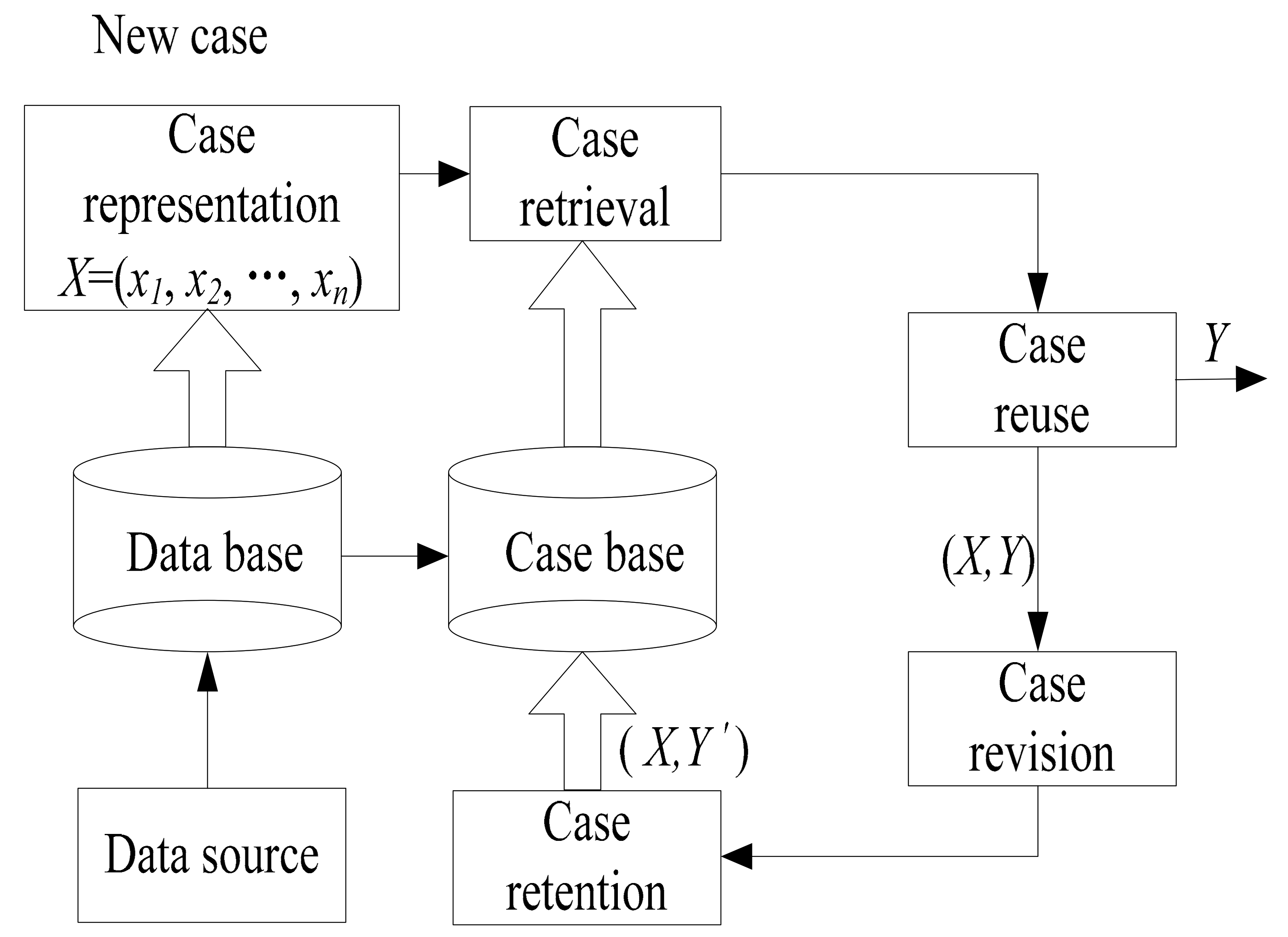
The basic CBR is composed of 4R procedures, namely, case retrieval, case reuse, case revision, and case retain. In the case of retrieval, the weight allocation of the case attribute determines the similarity between cases, thus affecting the result of case retrieval [20,21]. Due to the different characteristics of practical fields, the specific case-based reasoning model is not applicable to other application fields; moreover, the reasoning algorithm must not only meet the application model requirements of the actual system, but also be able to make it practical. Weight calculation for case similarity is a key issue of the CBR method. Algorithms for weight allocation must be improved or re-considered according to the case base of a certain field. It is necessary to set weights for the cases in these case libraries through fast and effective algorithms. Simulated annealing (SA) algorithm is a kind of optimization algorithm that converges to the optimal global solution with a probability of 1 [22,23]. SA has the adaptability to deal with both discrete data and continuous data. SA has the characteristics of universal, easy to achieve, and high quality, and is widely used in engineering fields, such as fault diagnosis, circuit design, vehicle routing, and image processing [23,24,25,26,27]. It is of high practical value. To make GSV PHM structure more suitable and practical, a CBR model containing a simulated annealing algorithm for optimizing case attribute weights is developed. The model begins with case representation, then, the optimization methods for attribute weights are established for case retrieval. The proposed method is applied to subsystem health evaluation of GSV. Cross-validation results show that the proposed method can reach the accuracy of case-based reasoning of GSV PHM structure.

The rest of this paper is organized as follows. In Section 2, the application framework using the CBR model for PHM is briefly introduced, as well as the topics regarding case representation, case retrieval, and case reuse are described. In Section 3, the optimization method of feature attribute weight allocation based on the SA algorithm is presented, which is developed in Java. Section 4 is application validation and design of comparative experiment in some data sets to evaluate the running performance of the application, and the results and analysis are provided as well. In Section 5, some conclusions and future outlooks are presented.

2. Framework Description

2.1. Data Construction and Module Development

2.1.1. Data Collection Process

In general, there are pressure detection unit, flow detection unit, temperature detection unit, voltage detection unit, displacement detection unit, and switch detection unit in the GSV. The data acquisition is as follows. Each detection unit collects information from sensors, encodes the information according to transmission protocol, and then sends the processed information to the central computer. Figure 1 shows the deployment of the data acquisition system.

We take the hydraulic control subsystem as an example to illustrate how to use the information collected by sensors to construct data for case analysis. Figure 2 shows one of the raw data acquisition deployments for the hydraulic control subsystem. Information about pressure and flow is acquired from sensors—the information is collected by the pressure detection unit and flow detection unit deployed in the vehicle. Following that, the information that contains raw data is received based on predefined format through the field bus network. Figure 3 shows the received information format. The information that contains raw data is decoded according to application protocol, and finally, processed data is stored in the database. Having historical data in the database, the following procedure is to create a case base using some function templates.

First, a class template is created.

Table 1. Class template for fault case definition.

Class Member	Definition and Description
id	identify case
name	The name of the failure case
symptom	Description of the fault phenomenon
time	time of the failure occurred
category	Categorize failure cases
flist-fname	Feature name
flist-ftype	Feature type
flist-fvalue	Feature value
flist-fweight	Feature weight

shows an example of a class template for fault case construction. In Table 1, a class template is used to construct the hydraulic control subsystem data set. Feature name and feature value is used to construct attribute-value pair.

Table 2. Example of case data from the hydraulic control subsystem.

Figure	Type	Parameter	Values of Record
Id	11	Primary key	11
YA1	int	Cylinder forth movement	3
YA2	int	Cylinder back movement	0
BF1	int	Digital relief valve 1 flow	11,598
BF2	int	Digital relief valve 2 flow	11,088
BP1	int	Main Pump Pressure	8320
BP2	int	Erect Pump Pressure	6491
YDL1	int	Front Support Pressure	240
YDL2	int	Back Support Pressure	240
TU30	double	Time (s)	33.947
FP	Varchar(255)	Fault mode	Spool abrasion

shows one record from the hydraulic control subsystem—in this record, eight attributes are extracted from the database, that is to say, cylinder forth movement (YA1), cylinder back movement (YA2), digital relief valve 1 flow (BF1), digital relief valve 2 flow (BF2), main pump pressure (BP1), erect pump pressure (BP2), front support pressure (YDL1) and back support pressure (YDL2), the corresponding value is (3, 0, 11,598, 11,088, 8320, 6491, 240, 240) for timestamp 33.947. Therefore, parameters of condition attributes are expressed as <YA1, YA2, BF1, BF2, BP1, BP2, YDL1, YDL2> = <3, 0, 11,598, 11,088, 8320, 6491, 240, 240>, these values are in the form of digital information and directly collected from the field bus network. These values must be converted into an analog quantity conversion according to the bus transmission protocol, so that the corresponding pressure, flow, and displacement can be obtained. Other attribute-value pair is processed in asimilar way. For each record, a conclusion is made to assess the operational behavior; the conclusion corresponds to solution attributes, solution attribute is in the form of discrete value or the probability in the range of (0,1). The discrete value indicates the positive or negative—in other words, normal state or abnormal state, probability indicates the degree of health performance of the system. In this way, condition attributes and solution attributes are determined for a case.

2.1.2. Logical Structure and Module

The basic reasoning process for the application is shown in Figure 4. It is noted that in the application, the database stores not only the raw data (unprocessed data from the data acquisition network), but also contains a mirror of the case base for safety purposes. This is based on the application requirement. After the case representation is completed, the case is saved in the database and mapped into the case base, and the case base is updated synchronously with the database. A basic routine for case reasoning is described as follows: Firstly, all attributes that correspond to the case are extracted from the case base, which is used to construct a field table. Secondly, a number of specific attributes are selected according to problem-solving requirement, which is used for similarity calculation. Finally, similarities between a source case and target case are calculated, and the most similar cases are found. With the weight optimization method, the target the case, based on the results of these similar cases, is reused or revised and saves it to the case base.

A software project named CBR Prosys is developed based on windows platform. The software realizes main function modules using java; the main function module includes attribute management, project management, case maintenance, case reasoning, and data monitoring. Each module not only has relative independence, but also contacts each other. This CBR system can be applied to different situations by the coordination among the four function modules. There are 37 classes altogether in the application. The design method is based on three-lay architecture, from top to bottom, it is GUI layer, logical business layer, and data access layer. Figure 5 shows the outline of the class module. Figure 6 shows a snapshot of the CBR process.

2.2. Case Representation

In case-based reasoning, the problem that is to be solved is usually referred to as the target case, the historical data or experience is called the source case, and each case is collected and stored in the database to form a case library. How to describe cases in a proper form is the premise of case-based reasoning. By using PHM structure, historical operating conditions of fault and health maintenance solutions are stored in a database. It is a raw knowledge base. The record in the knowledge base is either a text-based description or a sensor value and in the form of discrete format or numerical format. In order to establish the CBR model, the corresponding relationship between the operating conditions of the health maintenance solution must be extracted and converted into a case for storage to form a case base. That is to say, the method of case presentation is the premise. Some methods of case presentation, such as frame representation, the semantic network method, and the object-oriented method, can be found in the literature [28]. The simplest way to represent a case is by using attribute-value pairs, which is the property characteristic value description method. This way of representation is also beneficial for database storage.

In order to make the CBR method more practical and feasible for the mentioned PHM structure, the key indexes in the raw knowledge base are extracted to form a case attribute. In this paper, a single case contains condition attributes and solution attributes, condition attributes correspond to operational behaviors (problem description of the operational parameters), solution attributes correspond to health maintenance assessments (normal/abnormal, the degree of health status).

The general structure for the case base can be represented as $C=\left\{C_1,C_2,\dots ,C_n\right\}$, a single case $C_i$ in the case base can be expressed in two-tuples:

$$C_i: 〈X_i,Y_i〉,i=1,2, \dots ,n$$

(1)

In the above representation, n is the total number of cases, $X_i$ is condition attributes, and $Y_i$ is solution attributes. The representation of $X_i$ and $Y_i$ are expressed as follows:

$$X_i=\left(x_{i1},x_{i2},\dots ,x_{im}\right)$$

(2)

$$Y_i=\left(y_{i1},y_{i2},\dots ,y_{ip}\right)$$

(3)

where m and p is the total number of condition attributes for $X_i$ and solution attributes for $Y_i$, respectively.

The value of the condition attribute is continuously varying real numbers, or the value of attribute is discrete varying numbers. Therefore, different similarity calculation formulas need to be used. The calculation method of similarity is given in Section 2.3. The solution attribute can be a conclusion, which is used to indicate the positive (normal state) or negative (abnormal state). It can also be a probability of occurrence, which is used to describe the degree of health performance. As s result, the solution attribute will be reduced to $Y_i=(y_{i1})$, namely, one attribute is defined for $Y_i$.

2.3. Case Retrieval

Case retrieval is a key process in case reasoning. This step assures the right case is collected with a proper retrieval approach. In this paper, the k-nearest neighbor method is adopted to calculate case similarity between the source case and target case.

Let $C_i$ and $C_j$ denote ith case and jth case, respectively, then the similarity between the two cases can be calculated by using the similarity of their condition attributes, which can be described as below:

$$sim\left(C_i,C_j\right)={\left\{{\displaystyle \sum }_{q=1}^m{w}_q\times sim\left(x_{iq}, x_{jq}\right)\right\}}^{1/2}$$

(4)

Equation (4) is a modified weight Euclidean formula. $w_q$ is the weight of qth attribute. Attribute values that correspond to the feature are normalized to reduce the influence of different dimensions. Minimization-maximization is selected as the normalization method. The weight represents the importance of a condition attribute. The sum of each weight is 1, as below:

$${\displaystyle \sum }_{q=1}^m{w}_q=1$$

(5)

The greater the $sim〈C_i,C_j〉$ value, the higher the similarity between case $C_i$ and case $C_j$. The method of similarity calculation is dependent on the types of condition attribute format. If condition attribute format is continuously varying real numbers, the similarity is calculated as below:

$$sim\left(x_{iq},x_{jq}\right)=1-\left|x_{iq}-x_{jq}\right|,q=1,2,\dots , m$$

(6)

If condition attribute format is a discrete number, the similarity is calculated as below:

$$sim\left(x_{iq},x_{jq}\right)=\left\{\begin{array}{c}1;x_{iq}=x_{jq}\\ 0;x_{iq}\ne x_{jq}\end{array}\right.$$

(7)

where m is the total number of attributes,$1\le q\le m$. Through case retrieval, some of the source cases that are most similar to the target case can be selected. Then, the process of case reuse uses these selected similar cases to solve the target case. It uses the solutionattribute value of these selected cases to calculate the solution attribute value of the target case.

2.4. Case Reuse Model

After the case retrieval process is done, similar cases are selected. Case reuse is a process to solve target case based on these similar cases. This paper designs the rules of case reuse in two types of problems as below.

2.4.1. Solution Attribute with Two States

This is to determine the operation behavior of the vehicle. The solution attributes have only two states of “positive (normal)” and “negative (abnormal)”. The reuse of the case is described as follows:

The threshold value $\mathsf{\delta }$ of the case similarity is determined, and the source cases whose similarities exceed the threshold value $\mathsf{\delta }$ are selected. Suppose the total number of selected source cases is K, Remark the source cases whose solution attribute is ‘normal’ as positive cases, suppose the total number of positive cases is k. Finally, the solution attribute for target base is determined as below:

$$\eta =\frac{{{\displaystyle \sum }}_{i=1}^{k}si{m}_i^{+}}{{{\displaystyle \sum }}_{j=1}^{K}si{m}_j}$$

(8)

In Equation (8), the numerator represents the sum of case similarities between each positive case and the target case. The denominator is the sum of case similarity between each selected case and the target case. If $\eta >0.5$, solution attribute of the target case is positive, which indicates a normal state (no fault). Otherwise, the solution attribute of the target case is negative, which indicates an abnormal state; further operation of fault detection and diagnosis is recommended.

2.4.2. Solution Attribute with Probability Value

This is to describe the degree of health status, and is defined as a health predication problem. As mentioned above, the k-nearest neighbor method is used for case reuse. Suppose k source cases with the highest similarity to the target case are selected, and re-mark these selected case similarities as $si{m}_1,si{m}_2,\dots ,si{m}_k$, respectively. The solution attributes values of k selected source cases are marked as ${\mathrm{y}}_1,{\mathrm{y}}_2,\dots ,{\mathrm{y}}_{\mathrm{k}}$. Finally, the solution attribute of the target case is determined as below.

$$y={\displaystyle \sum }_{j=1}^k\frac{si{m}_j}{{{\displaystyle \sum }}_{i=1}^{k}si{m}_i}\times y_j$$

(9)

where $si{m}_j$ denotes the similarity between the jth case and the target case, and ${\mathrm{y}}_{\mathrm{j}}$ denotes the solution attribute value of the jth case. ${\sum }_{i=1}^{k}si{m}_i$ denotes the sum of similarity between each selected case and the target case.

3. Module of Weight Optimization

In the process of case retrieval, the weights should be allocated, so that importance for each attribute value reaches the optimized result. There are two kinds of weight allocation methods: The subjective method and objective method. The subjective method includes expert consultation method; factor paired comparison method, the minimum sum of squares method, and analytic hierarchy process, etc. [29]. Such weight allocation methods rely on human experience, which is subjective and uncertain. In order to overcome the subjective influence, some objective methods have been put forward. There are artificial neural network method, water injection theory method, and genetic algorithm method [30,31,32,33,34]. But these methods also have some shortcomings. The artificial neural network method calculates the feature weights according to the training model and its connection weight value, which is poor to explain, and hard to be transplanted [35,36]. The principle of the water injection method is based on data correlation, which is strict to the types of data. It would make a poor performance in some discrete data sets. The genetic algorithm tends to converge prematurely. The population size, cross-rate, and mutation rate of the genetic algorithm have a great influence on the solution, but the setting of parameter is neither uniform enough nor simple enough. From the viewpoint of practical purpose, simulated annealing algorithm has the characteristics of universal, easy to achieve. It is also easy to code and can generate better solutions. This is an attractive option for optimization problems where complex algorithms are not feasible, especially for application development of practical fields. In this paper, the SA method is employed and coded to optimize weight.

3.1. Basic Steps for Algorithm

The basic steps of the SA algorithm are developed as a function module, so the main procedure can call the module whenever necessary. The basic steps are given as follows.

Step 1. 

Initialize parameters: Temperature T, Temperature decreasing factor $\mathrm{\Delta }t$, current solution $W=\left(w_1,w_2,\dots ,w_m\right)$, $w_i\in \left(0,1\right), i=1,2,\dots ,m.$, repeat number L, minimum temperature $T_{min}$.

Step 2. 

For temperature T, repeat Step 3 to Step 5 for L times.

Step 3. 

Generate the new solution $\mathrm{W} \prime$ (Namely, the new weight vector in the feasible solution space is obtained based on the initial weight vector).

Step 4. 

Substitute the new solution $W^{\prime }$ into the case-based reasoning process, and calculate the increment $\mathrm{\Delta }F=F\left(W^{\prime }\right)-F\left(W\right)$. Where, $F\left(W\right)$ denotes the objective function of the SA algorithm. The calculation detail of the objective function is explained in Section 3.2.

Step 5. 

 If the increment of objective function is less than zero, the new solution is directly accepted as the current solution. Otherwise, the new solution is accepted as the current solution with probability $exp\left(-\frac{\mathrm{\Delta }F}{F}\right)$.

Step 6. 

If some termination condition is satisfied, the algorithm will stop, and the approximation of the optimal solution is output. Otherwise, go to Step 7.

Step 7. 

Decreasing temperature $T=T\times \mathrm{\Delta }t$. If T is less than $T_{min}$, the algorithm will stop. Otherwise go to Step 2, and continue the cycle.

3.2. Performance Index for Objective Function

In this application, a case library is established using the historical data record set. In order to improve the optimization effect of weights, a cross-validation method is adopted. The procedure is described as below.

At first, select n case from case library, and divide the selected n cases into five subsets, and the subsets are marked as $S^1$,$S^2$,$S^3, S^4$ and $S^5$, respectively. The total number of cases in each subset is equal. Mark one subset as the target case, and the remaining four subsets are combined to form the source case. The source case is the training set, and the target case is the test set. Following that, case retrieval and case reuse are implemented according to description in Section 2.4. Finally, the solution attribute value of each target case is obtained. Each subset in $S=\left\{S^1,S^2,S^3 ,S^4, S^5 \right\}$ will be taken as the target case in turn, and the remaining four subsets will form the source case base. This process repeats five times until the cross-validation is completed, the objective function is described as below.

(1)

 The selected case in the case library is expressed as Equations (1)–(3); for each case, there is more than one condition attribute and only one solutions attribute, and the value of the solution attribute can only be a normal state or abnormal state. The subsets from source cases are organized, as below.

$$S_j^i:〈X_j^i,Y_j^i〉$$

(10)

$$X_j^i=(x_{j1}^i,x_{j2}^i,\dots ,x_{jm}^i)$$

(11)

$$Y_j^i=y_{j1}^i$$

(12)

In Equations (10)–(12), $i=1, 2, 3, 4, 5.j=1, 2, \dots , G. x_{jm}^i$ denotes jth case has condition attribute of m in subset $S^i$, $y_j^i$ denotes jth case has 1 solution attribute of $y_1$ in subset $S^i$. $y_j^i$ can only be normal state or abnormal state. According to the description in Section 2.4.1, suppose the number of cases with correct state classification in the target case set is $G^c$, and the number of target cases is G, the state classification accuracy and state classification error is computed, as follows.

$${\mathrm{\Delta }}_i=\frac{G^c}{G}\times 100\%$$

(13)

$$e_i=1-{\mathrm{\Delta }}_i$$

(14)

where e_i denotes the percentage of misclassified cases in the target case set. The smaller the state classification error rate, the better the state classification accuracy. The objective function is setup by averaging the state classification error rate.

$$F\left(W\right)=\frac{1}{5}{\displaystyle \sum }_{i=1}^5{e}_i$$

(15)

(2)

 The selected case in the case library is expressed as Equations (1)–(3); for each case, there are more than one condition attribute and only one solutions attribute, and the value of the solution attribute is the probability value in the range of (0,1). The subsets from source cases are organized as the same in Equations (10)–(12), but the root mean square error is taken, as below.

$${\left(rmse\right)}_i={\left\{\frac{1}{G}{{\displaystyle \sum }}_{i=1}^G{\left(y_j^i-{\overline{y}}_j^i\right)}^2\right\}}^{1/2}$$

(16)

In the formula, $y_j^i$ represents the inference value of the solution attribute of the jth target case in subset $S^i$, and ${\overline{y}}_j^i$ represents its actual value. The smaller the RMSE, the better the result. Similarly, the objective function is setup by averaging the root mean square error.

$$F\left(W\right)=\frac{1}{5}{\displaystyle \sum }_{i=1}^5{\left(rmse\right)}_i$$

(17)

It can be seen from Equation (17) that the smaller the objective function, the better the attribute weight vector. Therefore, in the step of using the simulated annealing algorithm to obtain the feature attribute weight, the objective function can determine the optimized weight. If the objective function of the new solution becomes smaller, the new solution is directly accepted. Otherwise, the new solution is accepted with metropolis probability to jump out of the local optimum.

4. Application Validation and Analysis

4.1. Applicaiton Experiment Test

With the development of the application, function, and performance of the CBR reason model and optimization process must be evaluated to check if practical engineering requirement is satisfied. In this section, the application experiment is carried out by adopting historical data from GSV. Stored cases have been checked to reduce redundancy and to verify data validation. In the paper, the optimization method of even weight allocation CBR model (EW-CBR) and correlation coefficient weight allocation CBR model (CW-CBR) is also employed to make a comparison with the developed SA weight allocation CBR model (SA-CBR), and to check if the module functions properly.

In

Table 3. Data set for a normal and abnormal state.

Subset	Case Produced *	Number of Sample	Number of Attribute
A1	H	768	8
A2	H + F	267	22
A3	E	1372	4
A4	E + H	1000	12
A5	H + E + T	569	30

* H denotes hydraulic subsystem, T denotes temperature control subsystem, F denotes fixed aiming subsystem, P denotes power supply and distribution subsystem, Fc denotes fuel control subsystem, E denotes electric control subsystem, C denotes communication subsystem.

, $A_i$(i = 1, 2, 3, 4, 5) represents a subsystem or a combination of the subsystems, and the feature attribute includes the numerical value from the sensor (including eight pressure parameters, four temperature parameters, eight flow parameters, four voltage parameters, and four current parameters) and Discrete quantities (relay open/closed state, valve closed/closed state, communication identification state, gear switch, status indicator). For example, if the health status is judged from the hydraulic subsystem, only the feature attributes corresponding to the hydraulic subsystem are used. If the health status is comprehensively considered from the hydraulic subsystem and the temperature control subsystem, the corresponding feature attributes of both the hydraulic subsystem and the temperature control subsystem are used, the reasoning result will show if the system is normal or abnormal. Accordingly, in

Table 4. Data set for the degree of health performance.

Subset	Case Produced *	Number of Sample	Number of Attribute
B1	H	1030	8
B2	E	302	8
B3	F	103	9
B4	H + T	760	8
B5	P	1503	5

* H denotes hydraulic subsystem, T denotes temperature control subsystem, F denotes fixed aiming subsystem, P denotes power supply and distribution subsystem, Fc denotes fuel control subsystem, E denotes electric control subsystem, C denotes communication subsystem.

, the reasoning result will show the degree of health performance in the probability of (0, 1). The subset $B_i$(i = 1, 2, 3, 4, 5) has the same meaning as in Table 3. The case name denotes the subsystem or combination of the subsystem, in which H denotes hydraulic subsystem, T denotes temperature control subsystem, F denotes fixed aiming subsystem, P denotes power supply and distribution subsystem, Fc denotes fuel control subsystem, E denotes electric control subsystem, C denotes communication subsystem.

The basic process is as follows:

Step 1. 

Given initial weights, take one of the 5 subsets as the target case and the remaining four subsets as the source case, and calculate the similarity in turn.

Step 2. 

Determine the number of matching cases according to the similarity threshold and k-nearest neighbor. If it is met, go to step 3, if it does not match, go to step 4.

Step 3. 

Verify the case reuse result. If it meets the requirements, and the result is correct, go to Step 5. Otherwise, continue to step 4.

Step 4. 

Use SA-CBR, EW-CBR, and CW-CBR to optimize weight distribution as described in Section 4.1.1–Section 4.1.3, and return to step 3.

Step 5. 

Save the case, output the result, return to step 1, repeat five times.

4.1.1. Threshold of Case Similarity Determination

For the problem of normal/abnormal state determination, the case similarity threshold $\mathsf{\delta }$ mentioned in Section 2.4.1 will affect the number of cases selected in the case retrieval, thus affect the final inference result. Therefore, for each data set, the threshold value $\mathsf{\delta }$ is set to 0.75, 0.80, 0.85, 0.90, and 0.95, respectively. The case-based reasoning method with EW-CBR is used to obtain the state classification accuracy under adifferent threshold. The threshold $\mathsf{\delta }$ with the minimum state classification error of each data set is selected. The better threshold value $\mathsf{\delta }$ of each data set is shown in

Table 5. Threshold of case similarity.

Data Set	A1	A2	A3	A4	A5
$\mathsf{\delta }$	0.9	0.85	0.9	0.85	0.9

. The threshold listed in Table 5 is also used to compare the state classification problem in Section 4.1.3.

4.1.2. k Value Determination

For the problem of degree of health performance determination, the k-nearest neighbor method is adopted as described in Section 2.3, and the k value has an influence on the inference of results. Therefore, for each regression data set, k is set to 1, 3, 5, 7, and 9, respectively, with EW-CBR is employed. For each data set, calculate the RMSE for all candidate k values to determine the optimized k value for each data set. The obtained optimized k value is used as the comparison in Section 4.2. The optimized k value using the k-nearest neighbor method for each regression data set is shown in

Table 6. Value of k for each data set.

Data Set	B1	B2	B3	B4	B5
k	7	1	1	5	1

.

4.1.3. CBR Method for Comparison

Comparative analysis of weight allocation methods is carried to investigate the availability of the developed module using the CBR method for PHM structure. In order to further compare the proposed reasoning methods, CW-CBR is employed for comparison. The basic CW-CBR method taken in the paper is described as following.

(1)

 For the problem of normal/abnormal state determination, the solution attribute of the data set is processed to “1” and “0”, which represent the positive type and negative type. Then attribute weight is calculated according to the following formula.

$$w_i=S{R}_i/{{\displaystyle \sum }}_{i=1}^{m}S{R}_i$$

(18)

where $S{R}_i$ denotes the correlation degree between the ith condition attribute and the solution attribute Y.

(2)

For the problem of degree of health performance determination, the absolute value of the correlation coefficient between each condition attribute $X_i$ and solution attribute Y is calculated as below.

$$R_i=\left|\frac{Cov\left(X_i, Y\right)}{\sqrt{Var\left(X_i\right)\times Var\left(Y\right)}}\right|$$

(19)

where $Cov\left(X_i,Y\right)$ denotes the covariance of the ith condition attribute with solution attribute, Var denotes variance value. Suppose the number of attributes is m, then a attribute weight is calculated according to the following formula.

$$w_i=R_i/{{\displaystyle \sum }}_{i=1}^m{R}_i$$

(20)

For SA-CBR, the parameter settings are as follows: Starting temperature $T_{Start}=100$, temperature attenuation factor $T_{Weak}=0.92$, attribute weight disturbance step factor $Step=0.21$, Termination temperature $T_{Min}=0.001$, number of repetitions L = 2. If the current temperature is less than the minimum temperature, the algorithm will exit. For EW-CBR, the weight is the same value for all attribute, and the sum of weight equal to 1.

4.2. Results and Analysis

Based on the experimental application design mentioned above, the results are compared and analyzed. For each CBR method, a source case is constructed, and the source case is divided into five subsets. Cross-validation is carried out as described in Section 3. Using EW-CBR, CW-CBR, and SA-CBR methods to obtain attribute weights, respectively, and then the test cases are reasoned. For the problem of normal/abnormal state determination, the state classification accuracy is set as the evaluation index, and for the problem of degree of health performance, the root mean square error is set as the evaluation index. Finally, the inference results of the test cases are analyzed, as shown in Section 4.2.1 and Section 4.2.2.

4.2.1. Analysis on Result of Normal/Abnormal State Determination

In this case,

Table 7. State classification accuracy rate (%).

Subset	EW-CBR	CW-CBR	SA-CBR
A1	73.16	76.56	77.40
A2	69.65	68.16	74.57
A3	97.96	92.78	98.91
A4	70.89	72.90	75.20
A5	93.32	94.18	94.89

shows state classification accuracy for three CBR methods. It can be seen from the results that the state classification accuracy of the SA-CBR method is the highest, indicating that the SA-CBR method has the highest weight optimization ability. For data sets A1, A4, and A5, the state classification accuracy of CW-CBR is higher than that of EW-CBR, and it has certain weight optimization capabilities. For data sets A2 and A3, the state classification accuracy of CW-CBR are lower than that of EW-CBR. Therefore, the weighting method based on data correlation is not effective for state classification problems. Especially in the condition that the correlation of the data is not significant. Also, the result indicates that although for the same data set, the state classification accuracy of SA-CBR is as low as 74%, it is still higher than the accuracy obtained by the other two methods. Thus, SA-CBR is the first choice. Based on the engineering practice of the application, when the state classification accuracy is less than 70%, the result can only be used as a reference for operators. As we know, a single method is not always good for all circumstances, so we need to consider combining other optimization algorithms to develop more accurate models in the next step.

Furthermore, ROC diagrams of three weight allocation methods are given, which are especially suitable for the description and analysis of two-class problems [37,38], as shown in Figure 7a–e, respectively. In the above figures, the horizontal coordinate denotes the false positive rate (FPR), and the vertical coordinate denotes the true positive rate (TPR). FPR and TPR are calculations as follows.

$$TPR=TP/\left(TP+FN\right)$$

(21)

$$FPR=FP/\left(TN+FP\right)$$

(22)

where TP denotes the number of target cases whose result attribute is “positive” and are classified as “positive”. TN denotes the number of target cases whose result attribute is “negative” and are classified as “negative”. FP denotes the number of target cases whose result attribute is “negative” and are classified as “positive”. FN denotes the number of target cases whose result attribute is “positive” and are classified as “negative”.

Each point in the ROC graph represents a classifier, and the classifier reflects the pros and cons of classification performance. The closer the point is to the upper left corner (0, 1), the better the performance of the corresponding classifier, and the (0, 1) point represents the perfect classifier. It is easy to see from the ROC graphs of five data sets that SA-CBR has the best classification performance.

4.2.2. Analysis on Result of Degree of Health Performance Determination

In this case, the results obtained by the three methods are shown in Table 7, and the results are plotted in Figure 8. For the five data sets, the SA-CBR method is the smallest, indicating that the SA-CBR method has the strongest weight optimization ability. At the same time, except for data set B5, the RMSE value of the CW-CBR method is smaller than that of the EW-CBR method. CW-CBR has a certain weight optimization ability for numerical prediction problems, while EW-CBR has the worst reasoning effect.

From a comprehensive analysis, SA-CBR shows the best reasoning performance for both normal/abnormal state classification problem and health performance determination. In the problem of normal/abnormal state classification on data set A1 to A5, the state classification accuracy of this method increases by 4.24%, 4.92%, 0.95%, 4.31%, and 1.57%, respectively, compared to EW-CBR. In the problem of degree of health performance determination on data set B1 to B5, the root mean square error also decreases by 1.953, 1.559, 1.431, 0.328, and 0.328, respectively.

In summary, it can be seen from experimental results that for the allocation of feature attribute weights; SA-CBR is superior to the CW-CBR, while the CW-CBR is superior to EW-CBR. SA-CBR has the strongest weight optimization ability and can adapt to various types of data sets. SA-CBR has the highest reasoning accuracy in both normal/abnormal state determination and degree of health performance determination in the study. Although the CW-CBR has some capability of feature attribute weight optimization, it has some limitations on data set requirements. In some cases, it is not even as good as the EW-CBR method. Therefore, it can be inferred that the water injection principle method for weight distribution based on data correlation also has limitations.

5. Conclusions

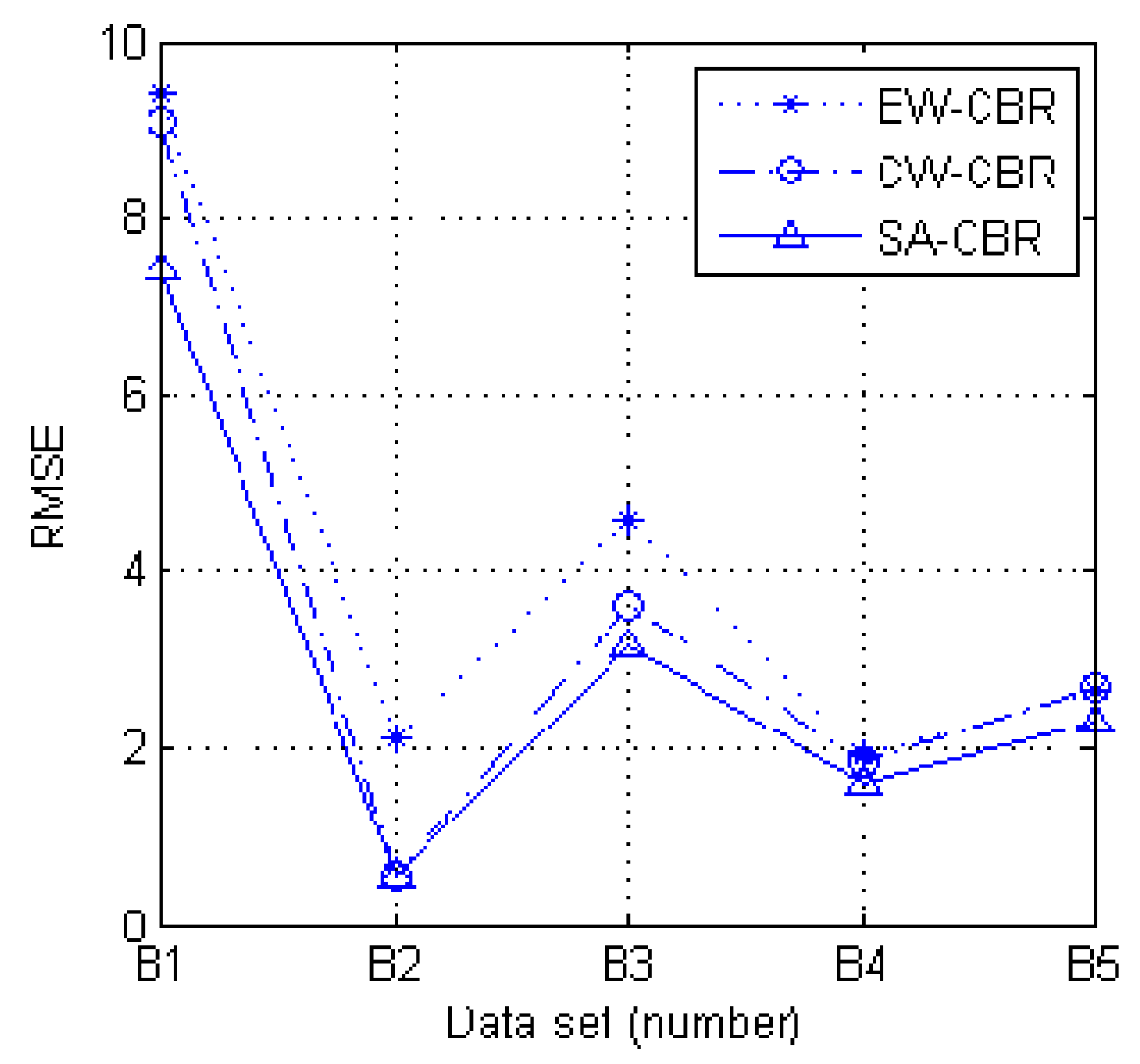
Through using data-driven health management processing and risk safety analysis in the PHM structure, this paper describes application development and establishes a CBR model to solve the normal/abnormal state determination and degree of health performance determination for practical purposes. In addition, the rules for case retrieval and case reuse have been established for state classification problems and health determination problems. In the weight distribution method, a feature attribute weight optimization method based on the simulated annealing algorithm is proposed. The proposed method combines case-based reasoning with machine learning and is a data-driven method. The developed SA-CBR module within the application uses historical cases to train feature attribute weights. The richer the historical data is collected, the more accurate the inference results will be. SA-CBR algorithm is simple and easy to understand, as well as parameter configuration is convenient; it is, therefore, practical for PHM structure. Three methods of EW-CBR, CW-CBR, and SA-CBR are investigated based on the actual historical data set, and experimental application results are shown and analyzed. The results indicate that validation of the developed SA-CBR module is simple to realize, and the practical requirement is satisfied.

Although the proposed method shows outstanding advantages, there are still many problems to be dealt with. At present, the established CBR model is specifically developed for the PHM structure of the launch vehicle system. In the future, it should be considered to be applied to more engineering fields. In addition, other methods can be introduced in the reasoning method to improve the reasoning performance. As the amount of historical data becomes larger and larger over time, simplifying redundant cases before reasoning is also a problem that needs to be considered.

References

1. Sheppard, J.W.; Kaufman, M.A.; Wilmer, T.J. IEEEStandards for Prognostics and Health Management. IEEE Aerosp. Electron. Syst. Mag. 2009, 24, 34–41. [Google Scholar] [CrossRef] [Green Version]
2. Niu, G.; Jiang, J.; Youn, B.D.; Pecht, M. Autonomous Health Management for PMSM Rail Vehicles through Demagnetization Monitoring and Prognosis Control. ISA Trans. 2018, 72, 245–255. [Google Scholar] [CrossRef] [PubMed]
3. Ardila, A.; Martinez, F.; Garces, K.; Barbieri, G.; Sanchez-Londono, D.; Caielli, A.; Cattaneo, L.; Fumagalli, L. XRepo—Towards an Information System for Prognostics and Health Mnagement Analysis. Procedia Manuf. 2020, 42, 146–153. [Google Scholar] [CrossRef]
4. Nguyen, D.V.; Kefalas, M.; Yang, K.; Apostolidis, A.; Olhofer, M.; Limmer, S.; Bäck, T.H. A Review: Prognostics and Health Management in Automotive and Aerospace. Int. J. Progn. Health Manag. 2019, 10, 1–35. [Google Scholar]
5. Liu, Z.; Jia, Z.; Vong, C.; Han, J.; Yan, C.; Pecht, M. A Patent Analysis of Prognostics and Health Management (PHM) Innovations for Electrical Systems. IEEE Access. 2018, 6, 18088–18107. [Google Scholar] [CrossRef]
6. Zhang, L.; Lin, J.; Liu, B.; Zhang, Z.; Yan, X.; Wei, M. A Review on Deep Learning Applications in Prognostics and Health Management. IEEE Access. 2019, 7, 162415–162438. [Google Scholar] [CrossRef]
7. Khan, S.; Yairi, T. A review on the Application of Deep Learning in System Health Managemen. Mech. Syst. Signal Process. 2017, 107, 241–265. [Google Scholar] [CrossRef]
8. Ishibashi, R.; Júnior, C.L. GFRBS-PHM: A Genetic Fuzzy Rule-based System for phm with Improved Interpretability. In Proceedings of the IEEE Conference of Prognostics and Health Management, Gaithersburg, MD, USA, 24–27 June 2013. [Google Scholar]
9. Watson, I.; Perera, S. Case-based Design: AReview and Analysis of Building Design Applications. AI EDAM 1997, 11, 59–87. [Google Scholar] [CrossRef]
10. Aamodt, A.; Plaza, E. Case-Based Reasoning: Foundational Issues, Methodological Variations, and System Approaches. AI Commun. 1994, 7, 39–59. [Google Scholar] [CrossRef]
11. Xu, L.D. Case based Reasoning. IEEE Potentials 1995, 13, 10–13. [Google Scholar] [CrossRef]
12. Jian, C.; Zhe, T.; Zhenxing, L. A Review and Analysis of Case-based Reasoning Research. In Proceedings of the International Conference on Intelligent Transportation, Big Data and Smart City, Halong Bay, Vietnam, 19–20 December 2015. [Google Scholar]
13. Díaz-Agudo, B.; Goel, A.K. Report on the 24th International Conference on Case-Based Reasoning Research and Development (ICCBR-2016). AI Mag. 2017, 38, 89–90. [Google Scholar] [CrossRef] [Green Version]
14. Asif, M.; Ahmed, J. A Novel Case Base Reasoning and Frequent Pattern based Decision Support System for Mitigating Software Risk Factors. IEEE Access. 2020, 8, 102278–102291. [Google Scholar] [CrossRef]
15. Xie, R.; Luo, M.; Chen, Z.; Liu, W. A Multi-CBR Algorithm Based on Comprehensive Evaluation for Operation Planning of Helicopter. IEEE Access. 2020, 8, 124110–124121. [Google Scholar] [CrossRef]
16. Zhang, K.; Luo, N.; Li, Y. STGA-CBR: ACase-based Reasoning Method Based on Spatiotemporal Trajectory Similarity Assessment. IEEE Access 2020, 8, 22378–22385. [Google Scholar]
17. Khosravani, M.R.; Nasiri, S.; Weinberg, K. Application of Case-based Reasoning in a Fault Detection System on Production of Drippers. Appl. Soft Comput. 2019, 75, 227–232. [Google Scholar] [CrossRef]
18. Khosravani, M.R.; Nasiri, S. Injection Molding Manufacturing Process: Review of Case-based Reasoning Applications. J. Intell. Manuf. 2020, 31, 847–864. [Google Scholar] [CrossRef]
19. Grabowik, C.; Kalinowski, K.; Krenczyk, D.; Paprocka, I.; Kempa, W. Application of Case-based Reasoning for Machining Parameters Selection. IOP Conf. Ser. Mater. Sci. Eng. 2016, 145, 1–8. [Google Scholar] [CrossRef] [Green Version]
20. Yan, A.; Zhang, K.; Yu, Y.; Wang, P. An Attribute Difference Revision Method in Case-based Reasoning and Its Application. Eng. Appl. Artif. Intell. 2017, 65, 212–219. [Google Scholar] [CrossRef]
21. Yan, A.J.; Qian, L.M.; Wang, P. A Comparative Study of Attribute Weights Assignment for Case-based Reasoning. Acta Autom. Sin. 2014, 40, 1896–1902. [Google Scholar]
22. Haznedar, B.; Arslan, M.T.; Kalinli, A. Optimizing ANFIS Using Simulated Annealing Algorithm for Classification of Microarray Gene Expression Cancer Data. Med. Biol. Eng. Comput. 2021, 59, 497–509. [Google Scholar] [CrossRef]
23. Wei, L.; Zhang, Z.; Zhang, D.; Leung, S.C. A Simulated Annealing Algorithm for the Capacitated Vehicle Routing Problem with Two-dimensional Loading Constraints. Eur. J. Oper. Res. 2018, 265, 843–859. [Google Scholar] [CrossRef]
24. Diedrich, A.; Feldman, A.; Perdomo-Ortiz, A.; Rui, A.; Kleer, J.D. Applying Simulated Annealing to Problems in Model-based Diagnosis. In Proceedings of the 27th International workshop on principles of diagnosis, Denver, CO, USA, 4–7 October 2016. [Google Scholar]
25. Yuan, J.; Chen, J.; Wang, L.; Zhou, X.; Xia, Y.; Hu, J. ARBSA: Adaptive Range-Based Simulated Annealing for FPGA Placement. IEEE Trans. Computer-Aided Design Integr. Circuits Syst. 2019, 38, 2330–2342. [Google Scholar] [CrossRef]
26. Mar’i, F.; Mahmudy, W.F.; Santoso, P.B. Hybrid Particle Swarm Optimization and Simulated Annealing for Capacitated Vehicle Routing Problem. In Proceedings of the International conference on sustainable information engineering and technology (SIET), Lombok, Indonesia, 28–30 September 2019. [Google Scholar]
27. Karasulu, B. An Approach Based on Simulated Annealing to Optimize the Performance of Extraction of the Flower Region Using Mean-shift Segmentation. Appl. Soft Comput. 2013, 13, 4763–4785. [Google Scholar] [CrossRef]
28. Shen, L.; Yan, H.; Fan, H.; Wu, Y.; Zhang, Y. An Integrated System of Text Mining Technique and Case-based Reasoning (TM-CBR) for Supporting Green Building Design. Build. Environ. 2017, 124, 388–401. [Google Scholar] [CrossRef]
29. Kim, S. Hybrid Forecasting System Based on Case-based Reasoning and Analytic Hierarchy Process for Cost Estimation. J. CivilEng. Manag. 2013, 19, 86–96. [Google Scholar] [CrossRef]
30. Karaman, A.; Çalışkan, E. Affective Factors Weight Estimation in Tree Felling Time by Artificial Neural Networks. Expert Syst. Appl. 2009, 36, 4491–4496. [Google Scholar] [CrossRef]
31. Yan, A.; Wang, W.; Zhang, C.; Zhao, H. A Fault Prediction Method that Uses Improved Case-based Reasoning to Continuously Predict the Status of a Shaft Furnace. Inf. Sci. 2014, 259, 269–281. [Google Scholar] [CrossRef]
32. Zhao, H.; Yan, A.J.; Wang, P. On Improving Reliability of Case-based Reasoning Classifier. Acta Autom. Sin. 2014, 40, 2029–2036. [Google Scholar]
33. Beddoe, G.R.; Petrovic, S. Selecting and Weighting Features Using a Genetic Algorithm in a Case-based Reasoning Approach to Personnel Rostering. Eur. J. Oper. Res. 2006, 175, 649–671. [Google Scholar] [CrossRef]
34. Huang, M.-L.; Hung, Y.-H.; Lee, W.-M.; Li, R.K.; Hao, T. Usage of Case-Based Reasoning, Neural Network and Adaptive Neuro-Fuzzy Inference System Classification Techniques in Breast Cancer Dataset Classification Diagnosis. J. Med. Syst. 2010, 36, 407–414. [Google Scholar] [CrossRef]
35. Khorani, V.; Forouzideh, N.; Nasrabadi, A.M. Artificial neural network weights optimization using ICA, GA, ICA-GA and R-ICA-GA. Comparing performances. In Proceedings of the 2011 IEEE Workshop On Hybrid Intelligent Models And Applications, Paris, France, 11–15 April 2011. [Google Scholar]
36. Yan, A.; Dai, X.; Shao, H.; Wang, P. Self-organization Membrane Computing-based Attribute Weights Optimization for Case-based Reasoning Model. J. Beijing Univ. Tech. 2017, 43, 745–753. [Google Scholar]
37. FlachPeter, A. ROC Analysis. In Encyclopedia of Machine Learning and Data Mining; Springer: Boston, MA, USA, 2016. [Google Scholar]
38. Fawcett, T. An Introduction to ROC Analysis. Pattern Recognit. Lett. 2005, 27, 861–874. [Google Scholar] [CrossRef]
Figure 1. Topology of the data acquisition system.
Applsci 11 04494 g001
Figure 2. Cylinder and pump in the hydraulic control system.
Applsci 11 04494 g002
Figure 3. Information received from field bus network.
Applsci 11 04494 g003
Figure 4. The proposed logical structure.
Applsci 11 04494 g004
Figure 5. Outline of the class module.
Applsci 11 04494 g005
Figure 6. A snapshot of the CBR process.
Applsci 11 04494 g006
Figure 7. Comparison of the ROC diagram.
Applsci 11 04494 g007aApplsci 11 04494 g007b
Figure 8. Results of the comparison of three CBR methods.
Applsci 11 04494 g008