Article

Bayesian Feature Fusion Using Factor Graph in Reduced Normal Form

by
Amedeo Buonanno
1,*,
Antonio Nogarotto
2,
Giuseppe Cacace
2,
Giovanni Di Gennaro
2,
Francesco A. N. Palmieri
2,3,
Maria Valenti
1 and
Giorgio Graditi
4
1
Department of Energy Technologies and Renewable Energy Sources, Research Centre of Portici, ENEA, 80055 Portici, Italy
2
Dipartimento di Ingegneria, Università degli Studi della Campania “Luigi Vanvitelli”, Via Roma, 81031 Aversa, Italy
3
CNIT-Consorzio Nazionale Interuniversitario per le Telecomunicazioni, Complesso Universitario di Monte S. Angelo, Edificio Centri Comuni, Via Cintia, 80126 Naples, Italy
4
Department of Energy Technologies and Renewable Energy Sources, Research Centre of Casaccia, ENEA, Via Anguillarese, S. Maria di Galeria, 00123 Rome, Italy
*
Author to whom correspondence should be addressed.
Appl. Sci. 2021, 11(4), 1934; https://doi.org/10.3390/app11041934
Submission received: 8 December 2020 / Revised: 16 February 2021 / Accepted: 17 February 2021 / Published: 22 February 2021
(This article belongs to the Special Issue AI, Machine Learning and Deep Learning in Signal Processing)

Abstract

:
In this work, we investigate an Information Fusion architecture based on a Factor Graph in Reduced Normal Form. This paradigm permits to describe the fusion in a completely probabilistic framework and the information related to the different features are represented as messages that flow in a probabilistic network. In this way we build a sort of context for observed features conferring to the solution a great flexibility for managing different type of features with wrong and missing values as required by many real applications. Moreover, modifying opportunely the messages that flow into the network, we obtain an effective way to condition the inference based on the different reliability of each information source or in presence of single unreliable signal. The proposed architecture has been used to fuse different detectors for an identity document classification task but its flexibility, extendibility and robustness make it suitable to many real scenarios where the signal can be wrongly received or completely missing.

1. Introduction

Data Fusion techniques are becoming increasingly important in many application contexts, such as defence, energy, biomedicine, manufacturing, etc. Fusion methods lead to better understanding of a phenomenon and of the decisions to be taken, especially in terms of robustness and accuracy with respect to what we would obtain using separate sources of information [1].
We can identify three increasing abstraction levels of Data Fusion models: Data Level, Feature Level and Decision Level. Dasarathy [2] has proposed five fusion modes: Data In–Data Out (DaI-DaO) Fusion, Data In–Feature Out (DaI-FeO) Fusion, Feature In–Feature Out (FeI-FeO) Fusion, Feature In–Decision Out (FeI-DeO) Fusion, Decision In–Decision Out (DeI-DeO) Fusion.
In this work, we investigate the application of a Bayesian approach to the FeI-DeO Fusion, which can be considered one of the most common fusion paradigms. The input features, coming from different sensors, are merged to produce a more informed decision. The data, retrieved from each sensor, can have missing, or wrong values, and the proposed Bayesian approach permits to manage them in a robust and flexible way.
In the following, we apply the Bayesian Data Fusion methodology to the Classification of Documents in a Maritime Port scenario, limiting our attention to documents such as Passports, Identity Cards and Fiscal Codes from different countries.
The general architecture of such system is similar to Automated Border Control (ABC) [3], which is a self-service barrier that permits the identification of the passengers through the comparison between biometrics information stored in the passport’s chip and the face, fingerprint, or iris (or a combination of them). These automatic systems have improved the efficiency, rapidity and security of the identification process. A simplified scheme of an ABC is presented in Figure 1.
In our applications, each document is scanned in its front and back, and three specialized detectors extract face, text, and barcode, possibly present in it. The related content is also stored for a Document Verification, or for other steps of the overall Border Control as: Authenticity Check, Identity Verification, etc.
The document classification has been emerging as an important task for its application in several real scenarios where a huge number of documents has to be managed. In this context, many different solutions have been proposed that use the layout, the contained text, the visual contents or a combination of them as the more recent solutions [4,5]. In the recent years some approaches based on the Graph Convolutional Networks have demonstrated to be very promising [6,7] given their capability to describe the relations among different part of the document.
The identity document classification can be considered a particular type of more generic document classification task but the layout is not discriminant enough because the identity documents have similar layouts, the textual information is not so easy to extract and the available datasets are small and with critical privacy and legal issues. In the years the identity document classification task has been tackled using different approaches. Some solutions have used the visual features extracted from the document image itself in order to train a classifier [8,9]; other works have used the template matching approach comparing the observed document with some reference models [10]; finally different deep learning approaches have been investigated as [8,11,12].
In our work, instead of focusing on the strength and weakness of the particular classifiers and/or features, we describe a general architecture where information from different detectors (in general feature extractors or different classifiers), are fused together in order to infer the type of the presented document. The technique is based on the Naive Bayes model represented as Factor Graph in Reduced Normal Form (FGrn) [13]. Even though there is a vast literature on the application of Naive Bayes to the classification task and for the decision fusion [14,15], the usage of FGrn paradigm, confers to the proposed architecture more flexibility, extendibility and robustness in an unified probabilistic framework.
This work has been inspired by works on probabilistic context analysis [16,17]. In one of our previous works [18], we demonstrated that the context is a very valuable information to help complete or correct some available evidence. In this work we demonstrate that the presented model builds a sort of context for the measures, which reduces the uncertainty and improves the robustness of the overall system.

2. Materials and Methods

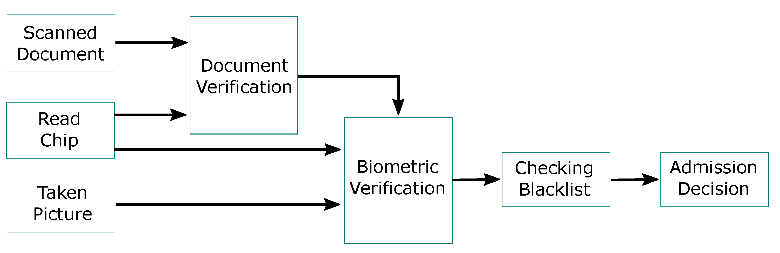
2.1. Model Architecture

For each document, we have at maximum one image for each side: front and back. Each image is presented to three detectors: Face Detector, Text Detector and Barcode Detector. Each detector returns, if it exists, the bounding box containing the object of interest: face, text and barcode.
We focus on simple features, i.e., the ratio between Area in Detected Bounding Box and the Area of the complete image. More complex features as CNN Features, SIFT or feature based on words extracted from the documents, could be used, but here we are focusing on the general fusion model and not so much on the best single features.
Moreover, the proposed approach permits to treat some situations that can occur in a real scenario, when some detections can be missing or wrongly transmitted and when some detectors, or detections, are more reliable than others.

2.1.1. Face Detector

The face detection has been implemented using YOLOv3 model [19], i.e., a deep neural network of 106 layers where the first 53 layers, called Darknet-53 and derived by Darknet-19 introduced in [20], are used as feature extractor. The major novelty of the YOLOv3, respect to the previous versions, is the capability of making detection on three different scales following the idea behind the feature pyramid paradigm [21]. YOLOv3 predicts 3 bounding boxes for each cell into which the image is divided. Each bounding box is described by 5 + Y C parameters: two center coordinates, two dimensions, the objectness score (that express how confident is the model that that box contains an object) and a classification vector that describes the classification confidence for each of Y C considered class.
For our face detection problem, we used weights of a pretrained architecture on WIDER FACE Dataset [22] available at [23], where the only class of interest is “face”.

2.1.2. Text Detector

Text detection has been implemented using the East model [24] with the pretrained weights available at [25]. East’s peculiarity is its ability to perform accurate detection on images that are not perfectly centered and rotated. The model is composed by three parts: the feature extractor, the feature merger and the predictor. The detected geometry is represented as a rotated box (R-BOX), consisting of four distances from the top, right, bottom, left boundaries of the rectangle and a rotation angle. The final step is the Non-Maximum Suppression algorithm, which avoids multi-detections of the same object.

2.1.3. Barcode Detector

Barcode detection was implemented using the Computer Vision algorithm adapted from [26]. The detector does not work with all existing barcodes, but it works well with those with a striped spectrum as ones present on identity cards and maritime documents. The input image is converted in grayscale and filtered using Scharr operator (with a 3 × 3 kernel) to detect the second derivative in the horizontal and vertical direction. The gradient image is filtered with a 9 × 9 blurring filter and a binary thresholding algorithm is applied in order to create a black and white image, where the white region contains the barcode. Morphological operations are also applied to make the candidate region more regular. Finally, if a detection exists, the boundaries of the barcode region are determined and the detector returns the coordinates of the bounding box.

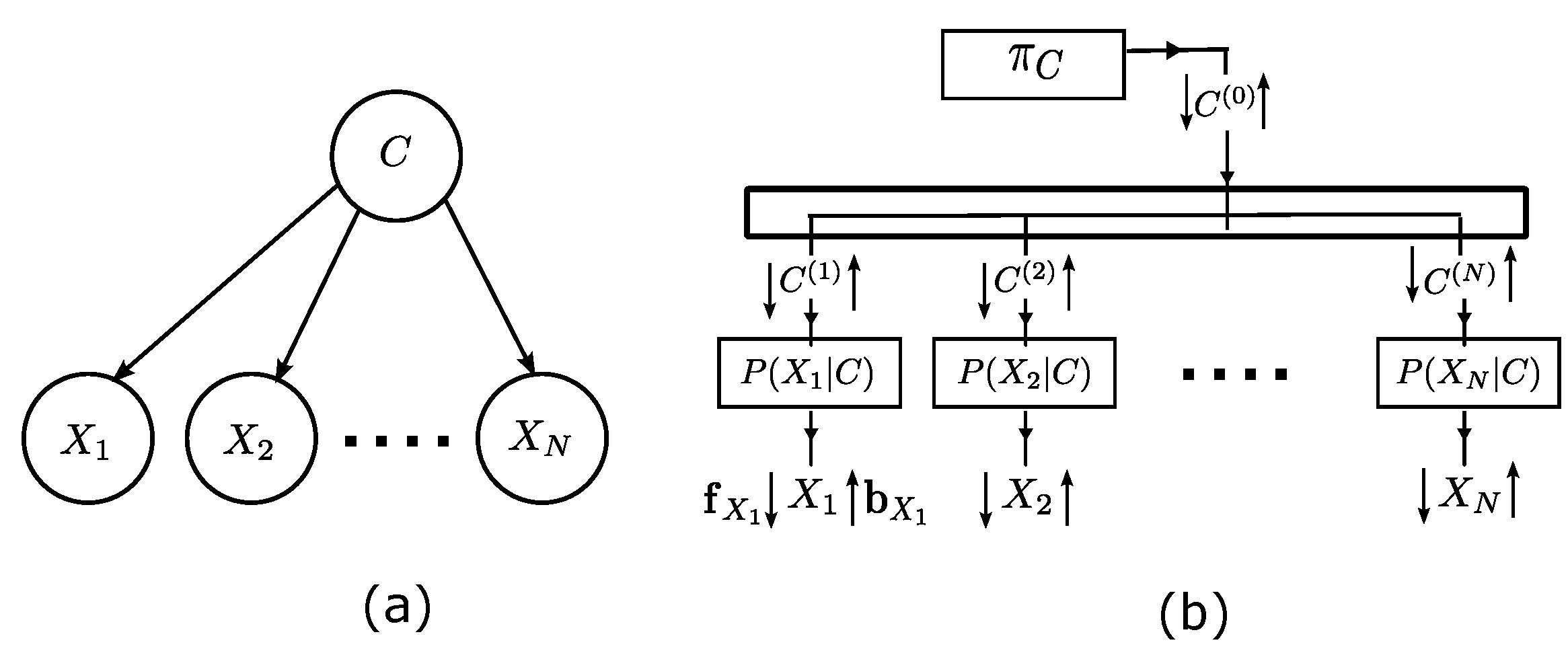
2.2. Feature Fusion Model

The proposed feature fusion architecture is based on the Naive Bayes model where N observed categorical variables { X 1 , X 2 , . . . , X N } are connected to a single class variable C.
Each observed variable represents the output of a sensor, detector or, more in general, an information source that need to be fused together with the other ones. It assumes values in a discrete alphabet: X i = { ξ 1 i , ξ 2 i , . . . , ξ L i i } ; where the dimension L i is the number of values that each variable can assume, if discrete, or the number of levels we use to quantize it (and which is therefore generally different for each variable). For the continuous variables several quantization schemes may be used, but here we propose a simple approach: the values assumed by each X i are clipped in [ m X i , M X i ] , where m X i and M X i are, respectively, the minimum and maximum permitted value for variable X i . The range is then divided uniformly using L i levels, so that the generic continuous value v is associated with level l if ( l 1 ) < v l .
It should be noted that in an Internet of Things (IoT) context, the number of levels used to quantize the sensor measure may be an important design parameter. In fact, generally, the trade-off between accuracy and available hardware resources need to be evaluated, for every specific application, also in terms of overall system energy consumption [15].
Finally, in the training phase, each variable X i is represented through a discrete distribution obtained using a smooth one-hot encoding. More specifically, for representing the k-th value of X i ( ξ k i ), instead of use a sharp distribution δ k i (an L i size vector representing the Kronecker delta, i.e., with all zero and only a one at the k-th position), we use a smoother distribution:
Applsci 11 01934 i001
where ϵ is a small positive number.
Since the values assumed by the detections are always positive, we set the minimum value m X i = M X i L i in order to “use” all L i levels. Differently, with m X i = 0 , the first quantization level will be underused since there are no negative values.
Furthermore, we assume that all observed variables are connected to one class variable C that assumes values in the discrete alphabet C = { γ 1 , γ 2 , . . . , γ L c } .
The relationship between each observed and class variable, is formalized by a Conditional Probability Table (CPT): P ( X i | C ) = [ P r { X i = x i | C = c } ] c C x i X i . This model is the classical Naive Bayes, shown in Figure 2 together with its FGrn representation, which represents the joint probability distribution:
p X 1 , X 2 , , X N , C ( x 1 , x 2 , , x N , c ) = π C ( c ) i = 1 N p X i | C ( x i | c )
where π C is the prior on C.
Please note that in the FGrn formulation the CPTs in Figure 2b are represented as Single Input-Single Output (SISO) blocks, making the model more flexible [13,27,28] with respect to other factor graph representation [29]. Learning each CPT is performed locally through backward and forward messages using the optimized Maximum Likelihood algorithm as described in [30]. The usage of FGrn provides us with a formal probabilistic framework for learning and allows easy handling of classification, error correction, missing values, etc.
In every single inference phase, when all observed variables are instantiated, the backward messages b X i = δ k i i are injected into the network, where k i is the index position of the instantiated value x ¯ i : = ξ k i i for the variable X i . In functional notation the backward message would be b X i ( x i ) = δ ( x i x ¯ i ) | x ¯ i X i , with i = 1 , , N . The class label is not observed and its forward message, f C , is set to a uniform distribution over class alphabet C .
After message propagation, the product of the backward and the forward messages at the class label ( b C ( c ) f C ( c ) ) is proportional to the posterior probability of the class given all the other instantiated observed variables, i.e.: b C ( c ) f C ( c ) = p X 1 , , X N , C ( x ¯ 1 , , x ¯ N , c ) p C | X 1 , , X N ( c | x ¯ 1 , , x ¯ N ) .
Suppose that all observed variables except one (e.g., X 1 ) are instantiated and that the class variable is unknown. Once we injected the messages in the network properly, after the message propagation we obtain:
f X 1 ( x 1 ) = c p X 1 | C ( x 1 | c ) p X 2 | C ( x ¯ 2 | c ) p X N | C ( x ¯ N | c ) π C ( c ) p X 1 | X 2 , , X N ( x 1 | x ¯ 2 , , x ¯ N )
in other words, the forward distribution of the non-instantiated variable is proportional to its posterior probability given all the other instantiated observed variables.
If also the class label is instantiated, the forward distribution of the non-instantiated variable (e.g., X 1 ), is proportional to its posterior probability given the class variable, i.e.: f X 1 ( x 1 ) p X 1 | C ( x 1 | c ¯ ) . This is coherent with the Naive Bayes model where each observed variable is conditionally independent from other variables given the class label.
The forward messages that we can collect at the observed variables represent the most probable configuration given the evidence and the learned model. Injected messages consistent with the forward values are considered plausible, while when this accordance is low an error, or a strange behavior, may have occurred.
We can also try to condition the behavior of the system based on the reliability (estimated or assumed) of each detector. If we have low confidence on a particular observed variable, X e , we can try to reduce its contribution raising the message b C ( e ) to an exponent 0 < ν < 1 and normalizing the resulting message. The effect of this operation is to make b C ( e ) ν more and more uniform with ν 0 , a sort of smoothing for the message. A uniform message does not make any contribution in the element-by-element product performed in the replicator block and successive normalization of the resulting message.
All the other messages b C ( i ) , with i { 1 , , N } { e } , can remain raised to 1 (no effect), or can be slightly augmented (raising to an exponent ν > 1 ) to weight more their contribution since the distribution thickens around the most probable value, a sort of sharpening for the message.

2.3. Model Evaluation

After the training phase, we can obtain classification results together with other inference over observed variable. Usually, in the classification problems, a confusion matrix that summarizes the classification performance of the trained model is computed. To take better into account the uncertainty in the answer, we present also the Jensen-Shannon divergence and Conditional Entropy on the class variable.

2.3.1. Likelihood

The likelihood for each example (observed variables) is available anywhere in the network. For example, the Likelihood for the n-th example of the X 1 variable is:
L X 1 [ n ] = c p X 1 , X 2 , , X N , C ( x ¯ 1 , x ¯ 2 , , x ¯ N , c ) = p X 1 , X 2 , , X N ( x 1 , x ¯ 2 , , x ¯ N ) δ ( x 1 x ¯ 1 ) f X 1 ( x 1 ) b X 1 ( x ¯ 1 )
The previous equation is true for each observed variable and it is always identical in every point of the network. The Likelihood computation can be performed for all examples of Training set and Test set.

2.3.2. Conditional Entropy

The capability of the system to provide sharp responses on class variable, given all observed variables, can be obtained considering the conditional entropy of C given all the others [31], which quantifies the uncertainty we have on C given the evidence:
H ( C | X 1 , , X N ) = x 1 , , x N , c p X 1 , , X N , C ( x 1 , , x N , c ) log p C | X 1 , , X N ( c | x 1 , , x N ) : = x , c p X , C ( x , c ) log p C | X ( c | x )
Considering the n-th example, we can therefore compute the conditional entropy of C using messages as follows:
H ( C | X 1 = x ¯ 1 , , X N = x ¯ N ) = c p X 1 , , X N , C ( x ¯ 1 , , x ¯ N , c ) log p C | X 1 , , X N ( c | x ¯ 1 , , x ¯ N ) : = c p X , C ( x ¯ , c ) log p C | X ( c | x ¯ ) = c p X , C ( x ¯ , c ) log p X , C ( x ¯ , c ) p X ( x ¯ ) = c p X , C ( x ¯ , c ) log p X , C ( x ¯ , c ) + c p X , C ( x ¯ , c ) log p X ( x ¯ ) = c b C ( c ) f C ( c ) log b C ( c ) f C ( c ) + log p X ( x ¯ ) c b C ( c ) f C ( c ) if f C ( c ) is uniform = 1 | C | c b C ( c ) log b C ( c ) + 1 | C | ( log p X ( x ¯ ) + log | C | ) c b C ( c ) since b C ( c ) is normalized = 1 | C | c b C ( c ) log b C ( c ) + 1 | C | log p X ( x ¯ ) + 1 | C | log | C | c b C ( c ) log b C ( c ) + log p X ( x ¯ ) + log | C |
Since log p X ( x ¯ ) and log | C | are constant respect to c, we focus only on the first term. As Likelihood, we can average Conditional Entropy over the Training and the Test Set.

2.3.3. Jensen-Shannon Divergence

Since the confusion matrix is based on the MAP (Maximum a Posteriori) rule, some interesting behaviors (how wrong are the results, what are the situations where the output is completely uniform, etc.) may be invisible. For this reason, we evaluated the Jensen-Shannon (JS) divergence between b C ( c ) and f C ( c ) . The JS divergence is based on Kullback Laibler (KL) divergence but has the advantage to be symmetric. Suppose we have two distribution P and Q over the same set X , then the JS divergence is defined as J S ( P , Q ) = 1 2 K L ( P , M ) + 1 2 K L ( Q , M ) ; where M = 1 2 ( P + Q ) , and K L ( P , M ) and K L ( Q , M ) are respectively the KL divergence between P and M and Q and M.

3. Results

In this work, we test the Fusion Model for the identity documents classification task. We selected simple features that model the predominance of a particular object (Face, Text, Barcode) in a document. Each feature is the ratio between area of the detection and total area of the document. The six categorical random variables are: Face Front ( X F F ), Face Back ( X F B ), Text Front ( X T F ), Text Back ( X T B ), Barcode Front ( X B F ), Barcode Back ( X B B ). Each variable represents and takes values in its discrete alphabets: X F F , X F B , X T F , X T B , X B F , X B B of dimension, respectively, L F F , L F B , L T F , L T B , L B F , L B B . The dimension of each dictionary is the number of levels we use to quantize the ratios of interest and, generally, is not the same for all variables.
The continuous and positive values obtained from each detector has to be properly quantized in order to be treated from our model where each observed variable X { X F F , X F B , X T F , X T B , X B F , X B B } is categorical.

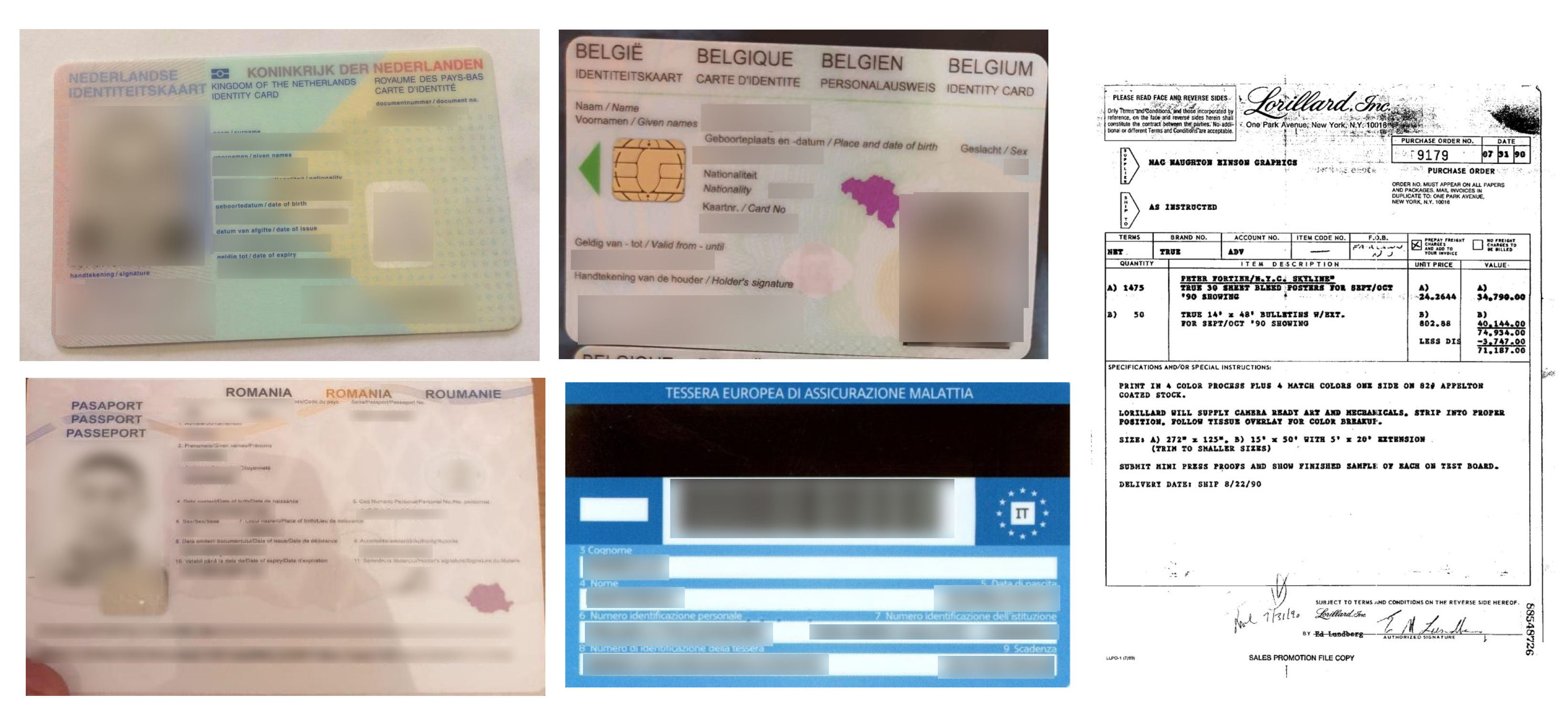
3.1. Dataset Preparation

Since privacy and legal issues, it is extremely difficult to access to a public dataset of identity documents. For this reason, we collected several identity documents from Internet adding 50 documents recorded in [32] and 36 private documents of some volunteers. The “other” documents are collected from Internet considering documents that could be related to the context of our interest and from RVL-CDIP Dataset [33], in particular from “invoice” and “form” categories.
In this way, we built a private dataset composed of 412 images representing personal documents: Fiscal Codes, Identity Documents, Driving License, Passports, and Other Images that can occur in the maritime application domain. The Driving License are then fused in the more general Identity Documents category.
For many documents (298) only the front pages are available and all the “back” variables ( X B B , X F B , X T B ) are missing. These examples have been excluded from the training process. The resulting 114 documents are distributed as follows: 29.8 % are Fiscal Codes (fc), 9.6 % are Identity Documents (id), 32.5 % are Passports (pa) and 28.1 % are Other documents (other). Since the document distribution is not related to the probability that a document is shown to the desk, the prior probability π C has not been learned and set to uniform over the 4 possible values. Table 1 contains the main characteristics of the considered dataset and the Figure 3 shows some examples.
Following what is described in Section 2.2, we set M X i to 95th percentile of the values present in the Training Set, L X i = 10 and m X i = M X i / 10 for each observed variable X i , except for the variable X B B which it is set to 75th percentile of the values present in the Training Set. The ϵ value is set to 10 5 .
After the quantization process a 5-fold Stratified Cross Validation procedure has been performed to assess the Classification Accuracy of the learned model. To have a fair evaluation of the model’s performance, at each split (after the quantization process based on the parameters defined from Training Set as described above), all duplicated records and records also present in the Training Set are removed from the Test Set. At this point we have backward messages for the observed variables and the same number of forward messages for the class variables. At each epoch the flow of messages in the network is used to learn the SISO blocks, with N s = 3 cycles and following the rules described in [13,28]. The learning process is stopped when all CPTs are unchanged and for a maximum of N e = 50 epochs. In Table 2 the confusion matrix for the dataset is shown together with per class precision, recall and F1-Score [34]. The overall classification accuracy is 82.7 % and the macro-average F1-Score (harmonic mean of the average precision and recall) is 0.8073 .

3.2. Inference

In the following paragraphs we present the results of some inference tasks based on a model trained on 80 records and tested on 22. The inference is performed injecting into the network the backward messages for the observed variables and collecting the backward messages at the class variable, comparing the resulting b C with the ground truth for the current example. Moreover the model responds with forward messages on the observed variables that is proportional, for each variable, to the posterior probability of the considered observed variable given all the other instantiated variables (Equation (2)). This is a sort of probability induced from the measure’s context represented by all evidences injected in the network.
Figure 4 shows the model’s answer when we inject the evidence related to an example: when the injected value is correct (upper row), when there is an error on X T F variable (middle row) and when the X T F variable is completely missing (lower row). It should be noted that both in missing and wrong cases, the model responds with the correct class, providing also with f X T F , that tries to correct, or complete the injected value since the suggested values are more consistent with the measure’s context.

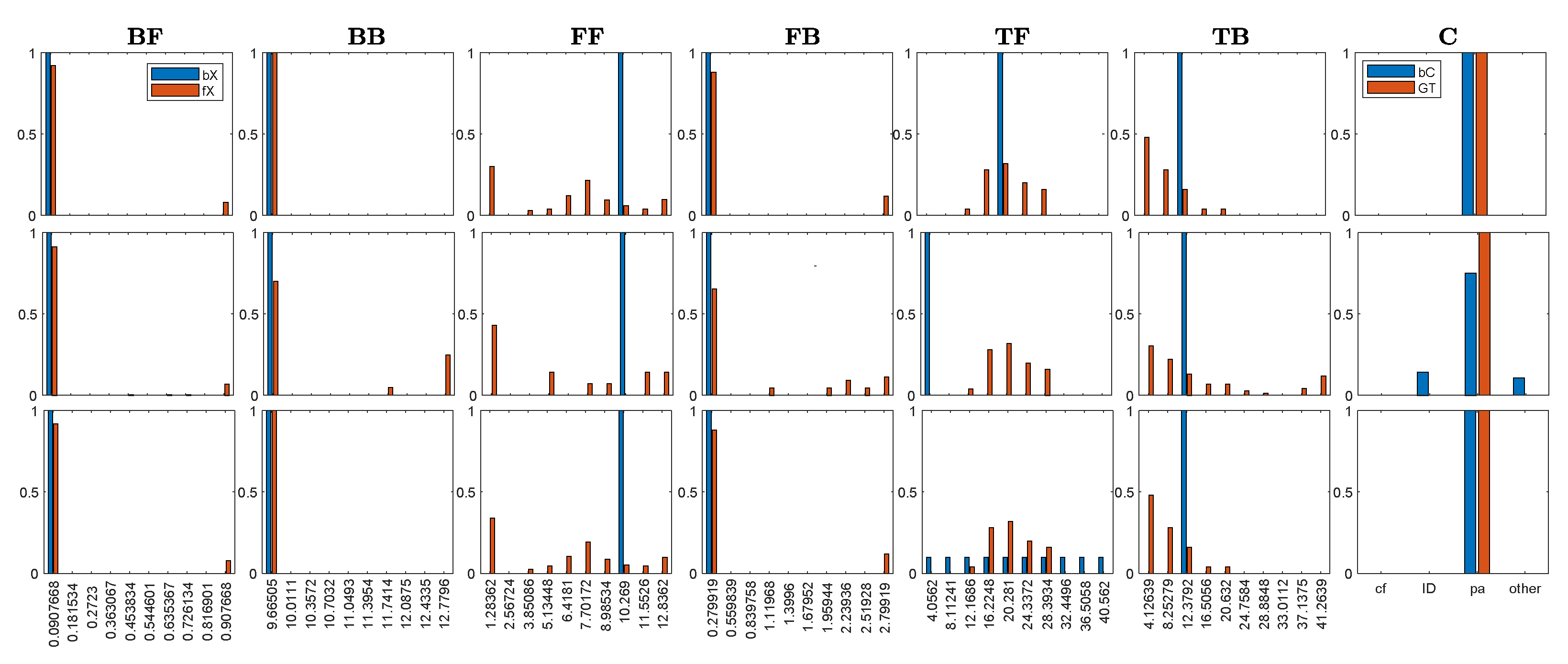
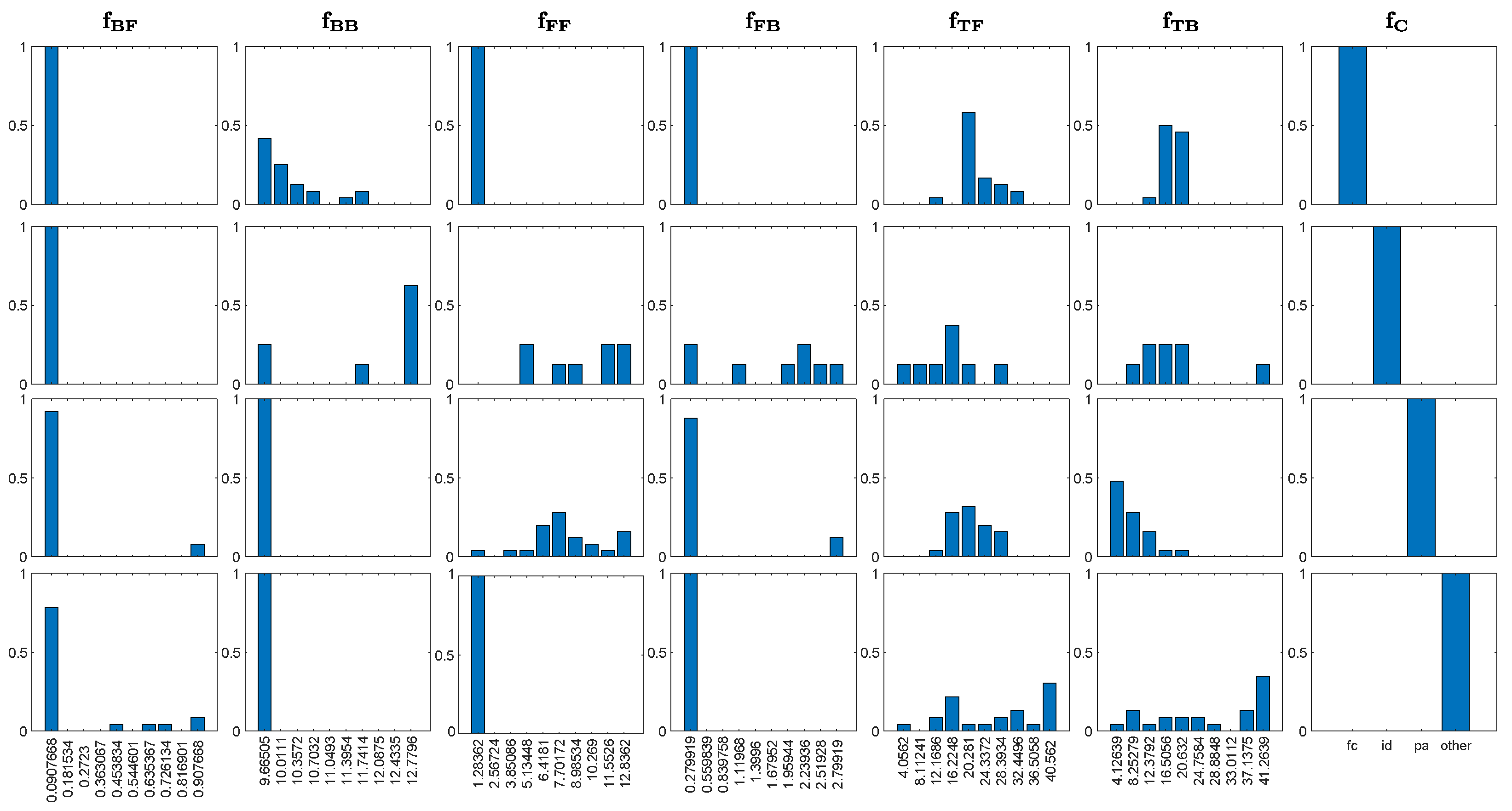
3.2.1. Measure’s Context

Figure 5 shows the model’s answer when we inject the evidence on the class variable ( f C ) and collect the forward messages on the observed variables ( f X i ) that represent the p X i | C ( x i | c ¯ ) . The distributions shown could be considered to be a context that can help the system in situation of high uncertainty, permitting, for example, to detect strange disagreement between the injected evidence and the system knowledge.

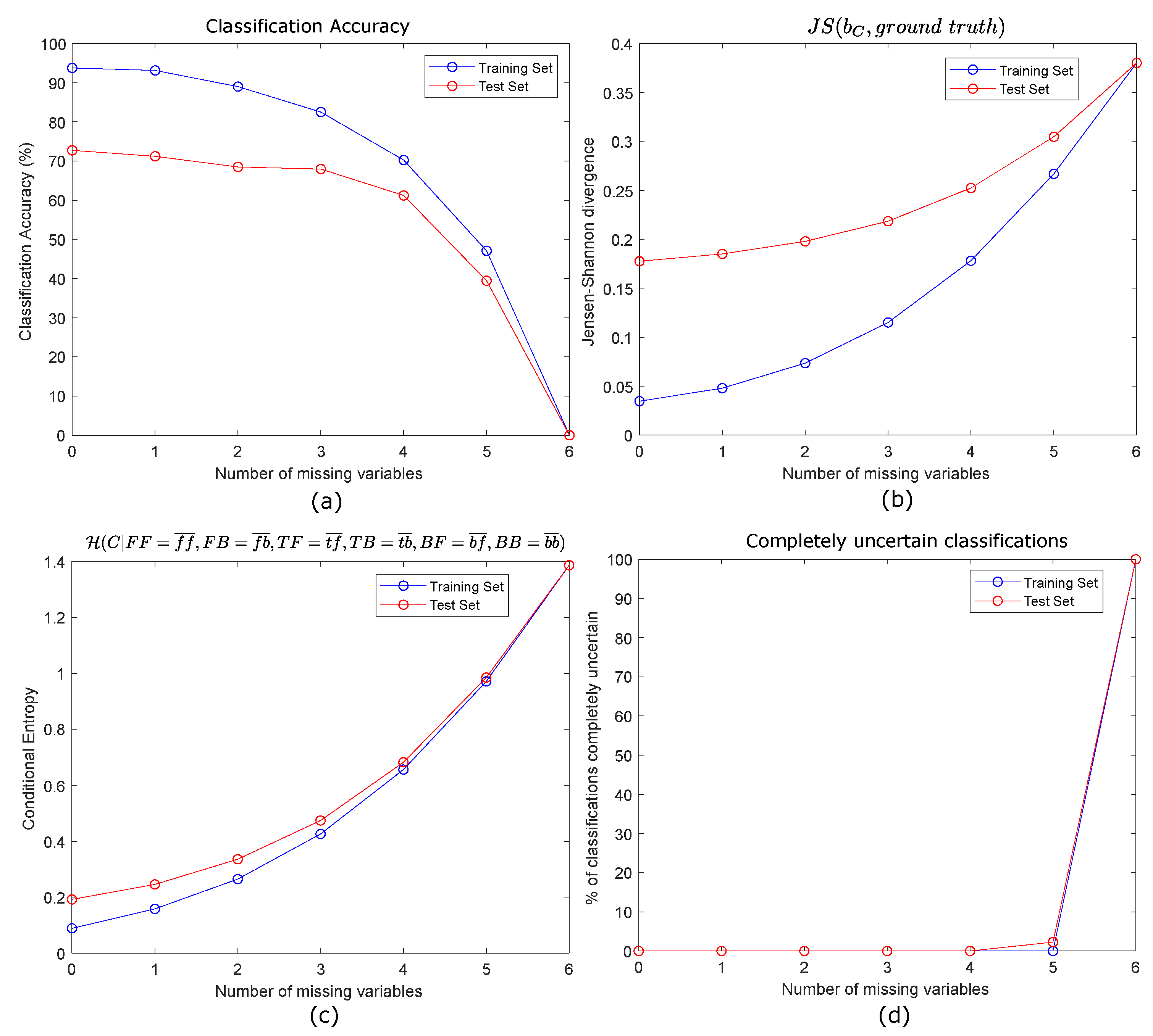
3.2.2. Missing Values’ Management

One of the most important characteristics of the Bayesian approach is its capability to treat missing values. In Figure 6 the effect of the absence of some detections on the classification performance is shown. All detections are correctly injected in the network except for k of them that are completely missing, and for which uniform distributions are injected in the network.
For increasing number of missing variables, we compute all the possible missing variables’ combinations and average the obtained metrics: classification accuracy, Jensen-Shannon Divergence and Conditional Entropy.
In Figure 6d we show also the number of completely uncertain classification that is always zero except for high number of missing variables. With all variable missing, we have a completely uncertain classification for all presented examples.
The graph demonstrates that, in the average, also with three completely missing detections (e.g., X F F , X F B , X T B or X F F , X T B and X B B , etc.) the classification accuracy decreases less than 10 % and also other metrics confirm the robustness of this model to the missing values. Please note that the Conditional Entropy describes an increasing in the uncertainty, in other words the classification becomes less sharp.
To emphasize the capability of the model to treat missing values, following the same procedure described in Section 3.1, we performed a 5-fold Stratified Cross Validation but, now, including the records with missing values in the Training Set and in the Test Set at each split (also in this case all duplicated records and records also present in the Training Set are removed from the Test Set). In Table 3 the confusion matrix is shown together with per class precision, recall and F1-Score. The overall classification accuracy is 76.2 % and the macro-average F1-Score is 0.7474 .
In the same configuration, if we do not take in account missing values in Training Set, we obtain a decrease in the accuracy classification ( 62.6 % ) and of the macro-average F1-Score ( 0.6506 ). This could suggest of including missing values also in the Training Set to increase the accuracy in presence of the missing values. Unfortunately, we can’t conclude this because the dimension of the effective Test Set for two simulations are different since, in the first case, several records in the Training Set are present also in the Test Set and hence are removed from it.
Moreover, we trained the model using all 114 records without missing values and performed a classification task only on the unique 80 records that contain missing values for the “back” variables ( X B B , X F B , X T B ). The classification accuracy for these records is 58.8 % and the macro-average F1-Score is 0.6274 . These simulations confirm the high flexibility and robustness of the model to manage missing values.

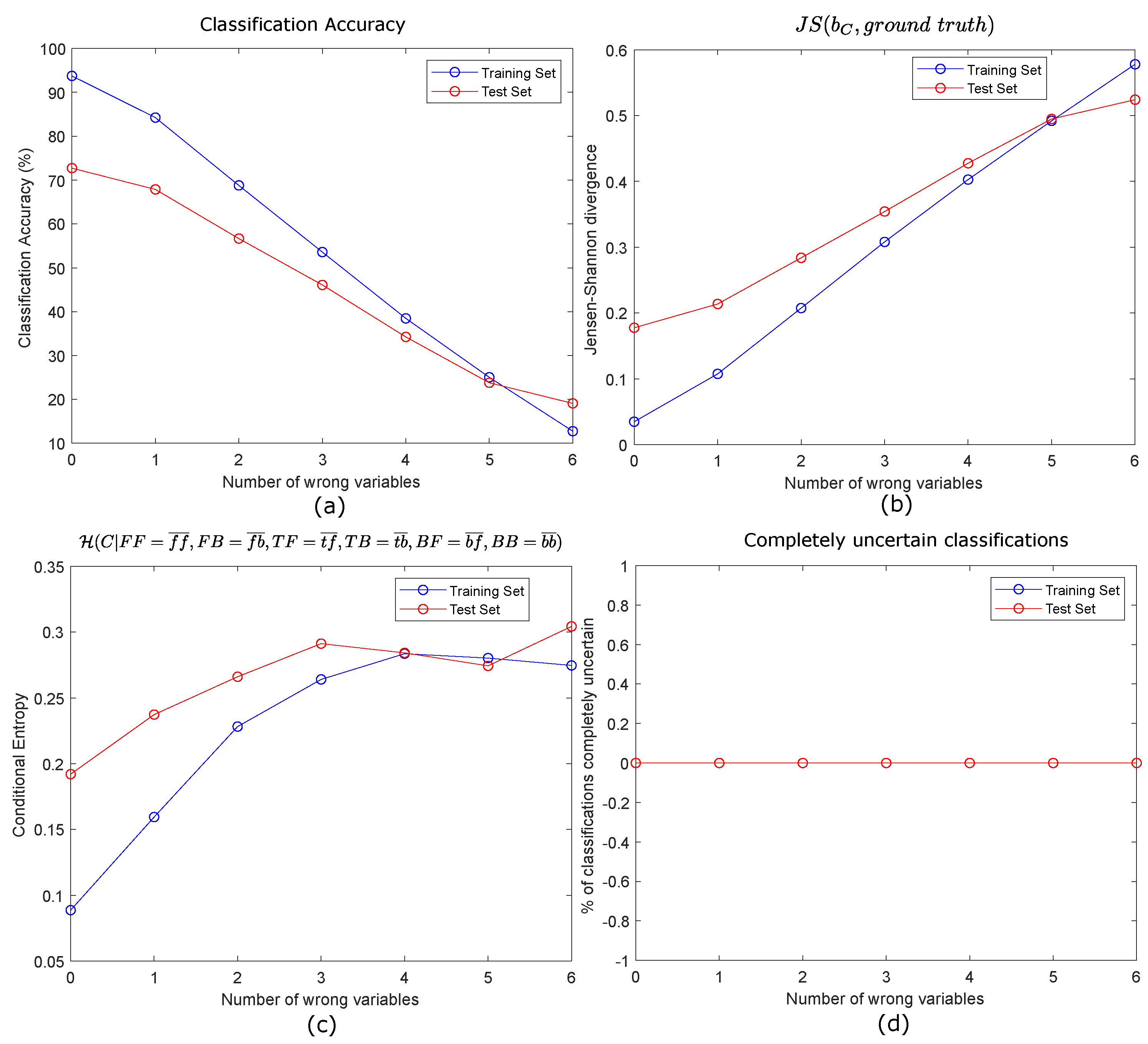
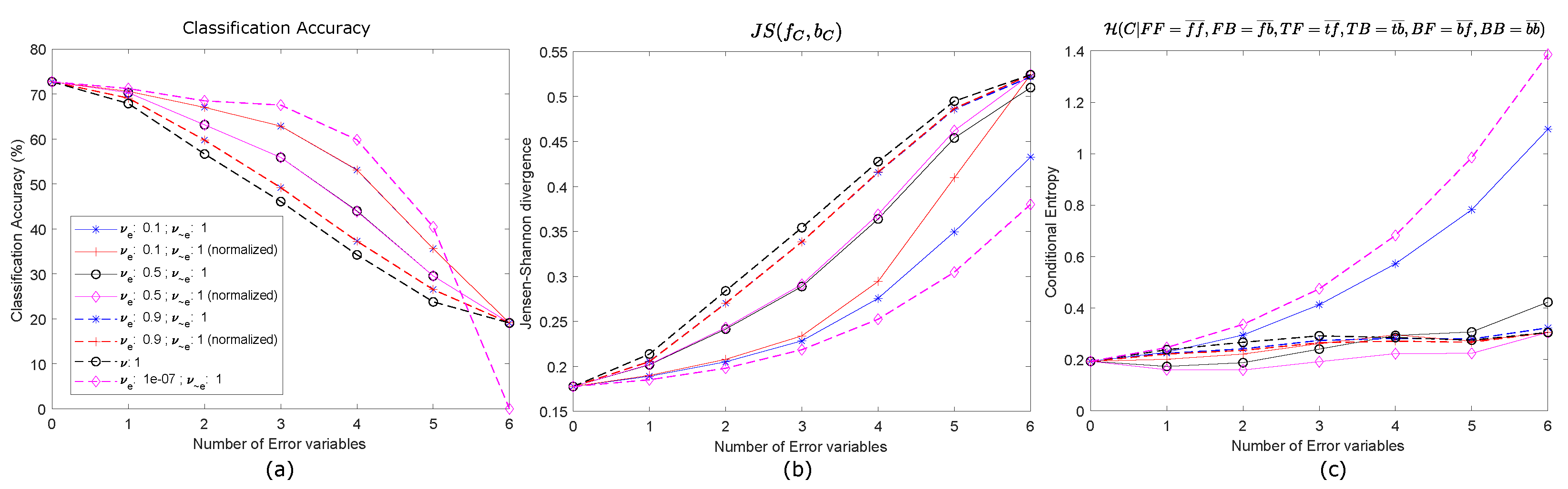
3.2.3. Errors Management

In Figure 7 the effect of the wrong detections on the classification performance is shown. In this simulation all detections are injected in the network but k of them are assumed to be completely wrong. For increasing number of wrong variables, we compute all the possible variables’ combinations and, for each combination, we insert 5 random detections for each variable using the smooth deltas. We let the messages flow in the network and average the obtained metrics: classification accuracy, Jensen-Shannon Divergence and Conditional Entropy. In Figure 7d we show also the number of completely uncertain classification. The graph shows how the system performance does not decrease too much for one wrong detection, but it decreases dramatically when more errors are inserted.

3.2.4. Reliability Test

As described in Section 2.2, the information coming from different devices has a reliability dependent on the confidence of the related detector. This reliability value can be assigned globally to a particular detector, or to a particular example, if we have evidence that the current one is not so accurate. In Figure 8 the effect of raising the messages b C ( e ) related to detectors containing errors, with an exponent ν e is shown. The exponent of messages related to other observed variables, i.e., not affected by errors, are indicated as ν e and are set to 1 (no effect) or “normalized”, in a way that the sum of all exponents is 6 with a sharpening effect on these variables:
ν e : = ν i | i e = N ν e N 1 = 6 ν e 5
As expected, with values of ν e extremely low ( 1 e 7 ) the trends are the same that in Figure 6, because the effect of such a small value for ν e is to delete completely the information related to a particular detector. The intermediate values of ν e instead, reduce the effect of the error improving the performance of system in terms of Classification Accuracy and Jensen-Shannon divergence.

4. Conclusions

In this work, we described an Information Fusion architecture using the Factor Graph in Reduced Normal Form paradigm.
The proposed approach permits learning a sort of measure’s context that, in presence of high uncertainty, helps to detect disagreement between the injected evidence and the system knowledge, giving to overall system great flexibility and robustness in the handling missing and wrong values. The proposed architecture, in fact, also in presence of missing values and errors, continues to have a good classification performance.
We also demonstrated how it is possible to condition the system in the presence of information sources with different reliability or in presence of single unreliable detection. This is another demonstration of the flexibility of the paradigm that can manage several information sources taking into account their peculiarities.
Even though the approach is completely general and applicable to several contexts where it is required to fuse information from several sources, the framework has been applied to a classification problem of identity documents, where different detectors are fused into a unique classifier.

Author Contributions

Conceptualization, A.B., G.D.G., F.A.N.P.; methodology, A.B., G.D.G., F.A.N.P.; software, A.B., A.N., G.C.; validation, A.B., G.D.G., F.A.N.P.; investigation, A.B., G.D.G., F.A.N.P.; data curation, A.N.; writing—original draft preparation, A.B.; writing—review and editing, A.B., A.N., G.C., G.D.G., F.A.N.P., M.V., G.G.; visualization, A.B., A.N.; supervision, A.B., F.A.N.P., M.V., G.G.; funding acquisition, F.A.N.P. All authors have read and agreed to the published version of the manuscript.

Funding

Work partially supported by POR CAMPANIA FESR 2014/2020, ITS for Logistics, awarded to CNIT (Consorzio Nazionale Interuniversitario per le Telecomunicazioni).

Data Availability Statement

The data are not publicly available due to privacy. The dataset of extracted features used in this study is available on request from the corresponding author.

Conflicts of Interest

The authors declare no conflict of interest. The funders had no role in the design of the study; in the collection, analyses, or interpretation of data; in the writing of the manuscript, or in the decision to publish the results.

References

  1. Raol, J.R. Data Fusion Mathematics: Theory and Practice; CRC Press: Boca Raton, FL, USA, 2017. [Google Scholar]
  2. Dasarathy, B.V. Sensor fusion potential exploitation-innovative architectures and illustrative applications. Proc. IEEE 1997, 85, 24–38. [Google Scholar] [CrossRef]
  3. Frontex. Best Practice Operational Guidelines for Automated Border Control (ABC) Systems; European Agency for the Management of Operational Cooperation at the External Borders of the Member States of the European Union; European Agency, 2012; Available online: https://www.scribd.com/document/169819829/Best-Practice-Operational-Guidelines-for-Automated-Border-Control (accessed on 1 November 2020). [CrossRef]
  4. Xu, Y.; Xu, Y.; Lv, T.; Cui, L.; Wei, F.; Wang, G.; Lu, Y.; Florencio, D.; Zhang, C.; Che, W.; et al. LayoutLMv2: Multi-Modal Pre-Training for Visually-Rich Document Understanding. arXiv 2020, arXiv:2012.14740. [Google Scholar]
  5. Bakkali, S.; Ming, Z.; Coustaty, M.; Rusiñol, M. Cross-Modal Deep Networks For Document Image Classification. In Proceedings of the 2020 IEEE International Conference on Image Processing (ICIP), Abu Dhabi, United Arab Emirates, 25–28 October 2020; pp. 2556–2560. [Google Scholar]
  6. Wang, Z.; Wang, C.; Zhang, H.; Duan, Z.; Zhou, M.; Chen, B. Learning Dynamic Hierarchical Topic Graph with Graph Convolutional Network for Document Classification. In Proceedings of the Twenty Third International Conference on Artificial Intelligence and Statistics (AISTAT) 2020, Online. 26–28 August 2020. [Google Scholar]
  7. Ullah, I.; Manzo, M.; Shah, M.; Madden, M. Graph Convolutional Networks: analysis, improvements and results. arXiv 2019, arXiv:1912.09592. [Google Scholar]
  8. Simon, M.; Rodner, E.; Denzler, J. Fine-grained classification of identity document types with only one example. In Proceedings of the 2015 14th IAPR International Conference on Machine Vision Applications (MVA), Tokyo, Japan, 18–22 May 2015; pp. 126–129. [Google Scholar] [CrossRef]
  9. Sicre, R.; Montaser Awal, A.; Furon, T. Identity documents classification as an image classification problem. In Proceedings of the ICIAP 2017—19th International Conference on Image Analysis and Processing, Catania, Italy, 11–15 September 2017; pp. 602–613. [Google Scholar] [CrossRef] [Green Version]
  10. Awal, A.M.; Ghanmi, N.; Sicre, R.; Furon, T. Complex Document Classification and Localization Application on Identity Document Images. In Proceedings of the 2017 14th IAPR International Conference on Document Analysis and Recognition (ICDAR), Kyoto, Japan, 9–15 November 2017; Volume 1, pp. 426–431. [Google Scholar]
  11. Vilàs Mari, P. Classification of Identity Documents Using a Deep Convolutional Neural Network. Master’s Thesis, Universitat Oberta de Catalunya, Barcelona, Spain, 2018. Available online: http://hdl.handle.net/10609/73186 (accessed on 4 December 2020).
  12. Ellena, F. Deep Convolutional Neural Networks for Document Classification. Master’s Thesis, Politecnico di Torino, Turin, Italy, 2018. Available online: http://webthesis.biblio.polito.it/id/eprint/7603 (accessed on 4 December 2020).
  13. Palmieri, F.A.N. A Comparison of Algorithms for Learning Hidden Variables in Bayesian Factor Graphs in Reduced Normal Form. IEEE Trans. Neural Netw. Learn. Syst. 2016, 27, 2242–2255. [Google Scholar] [CrossRef] [PubMed]
  14. Shi, X.; Manduchi, R. A Study on Bayes Feature Fusion for Image Classification. In Proceedings of the 2003 Conference on Computer Vision and Pattern Recognition Workshop, Madison, WI, USA, 16–22 June 2003; Volume 8, p. 95. [Google Scholar] [CrossRef] [Green Version]
  15. Olascoaga, L.I.G.; Meert, W.; Bruyninckx, H.; Verhelst, M. Extending Naive Bayes with Precision-Tunable Feature Variables for Resource-Efficient Sensor Fusion. In Proceedings of the 2nd Workshop on Artificial Intelligence and Internet of Things, Hague, The Netherlands, 30 August 2016; Volume 1724, pp. 23–30, AI-IoT@ECAI: 2016. [Google Scholar]
  16. Jin, Y.; Geman, S. Context and Hierarchy in a Probabilistic Image Model. In Proceedings of the 2006 IEEE Computer Society Conference on Computer Vision and Pattern Recognition (CVPR’06), New York, NY, USA, 17–22 June 2006; Volume 2, pp. 2145–2152. [Google Scholar] [CrossRef]
  17. Choi, M.J.; Torralba, A.; Willsky, A.S. A Tree-Based Context Model for Object Recognition. IEEE Trans. Pattern Anal. Mach. Intell. 2012, 34, 240–252. [Google Scholar] [CrossRef] [Green Version]
  18. Buonanno, A.; Iadicicco, P.; Di Gennaro, G.; Palmieri, F.A.N. Context Analysis Using a Bayesian Normal Graph. In Neural Advances in Processing Nonlinear Dynamic Signals; Esposito, A., Faundez-Zanuy, M., Morabito, F.C., Pasero, E., Eds.; Springer International Publishing: Cham, Switzerland, 2019; pp. 85–96. [Google Scholar] [CrossRef]
  19. Redmon, J.; Farhadi, A. YOLOv3: An Incremental Improvement. arXiv 2018, arXiv:1804.02767. [Google Scholar]
  20. Redmon, J.; Farhadi, A. YOLO9000: Better, Faster, Stronger. In Proceedings of the 2017 IEEE Conference on Computer Vision and Pattern Recognition (CVPR), Honolulu, HI, USA, 21–26 July 2017; pp. 6517–6525. [Google Scholar]
  21. Lin, T.; Dollár, P.; Girshick, R.; He, K.; Hariharan, B.; Belongie, S. Feature Pyramid Networks for Object Detection. In Proceedings of the 2017 IEEE Conference on Computer Vision and Pattern Recognition (CVPR), Honolulu, HI, USA, 21–26 July 2017; pp. 936–944. [Google Scholar] [CrossRef] [Green Version]
  22. Yang, S.; Luo, P.; Loy, C.C.; Tang, X. WIDER FACE: A Face Detection Benchmark. In Proceedings of the IEEE Conference on Computer Vision and Pattern Recognition (CVPR), Las Vegas, NV, USA, 27–30 June 2016; pp. 5525–5533. [Google Scholar]
  23. Nguyen, T. Yoloface. 2019. Available online: https://github.com/sthanhng/yoloface (accessed on 4 December 2020).
  24. Zhou, X.; Yao, C.; Wen, H.; Wang, Y.; Zhou, S.; He, W.; Liang, J. EAST: An Efficient and Accurate Scene Text Detector. In Proceedings of the IEEE Conference on Computer Vision and Pattern Recognition (CVPR), Honolulu, HI, USA, 21–26 July 2017. [Google Scholar]
  25. Argman. East. 2019. Available online: https://github.com/argman/EAST (accessed on 4 December 2020).
  26. Rosebrock, A. Detecting Barcodes in Images with Python and OpenCV. 2014. Available online: https://www.pyimagesearch.com/2014/11/24/detecting-barcodes-images-python-opencv/ (accessed on 4 December 2020).
  27. Buonanno, A.; Palmieri, F.A.N. Simulink Implementation of Belief Propagation in Normal Factor Graphs. In Advances in Neural Networks: Computational and Theoretical Issues; Bassis, S., Esposito, A., Morabito, F.C., Eds.; Springer International Publishing: Cham, Switzerland, 2015; pp. 11–20. [Google Scholar] [CrossRef]
  28. Buonanno, A.; Palmieri, F.A.N. Two-Dimensional Multi-layer Factor Graphs in Reduced Normal Form. In Proceedings of the International Joint Conference on Neural Networks, IJCNN2015, Killarney, Ireland, 12–17 July 2015. [Google Scholar]
  29. Koller, D.; Friedman, N. Probabilistic Graphical Models: Principles and Techniques—Adaptive Computation and Machine Learning; The MIT Press: Cambridge, MA, USA, 2009. [Google Scholar]
  30. Di Gennaro, G.; Buonanno, A.; Palmieri, F.A.N. Computational Optimization for Normal Form Realization of Bayesian Model Graphs. In Proceedings of the 2018 IEEE 28th International Workshop on Machine Learning for Signal Processing (MLSP), Aalborg, Denmark, 17–20 September 2018; pp. 1–6. [Google Scholar]
  31. Cover, T.M.; Thomas, J.A. Elements of Information Theory; Wiley: New York, NY, USA, 2006. [Google Scholar]
  32. Arlazarov, V.; Bulatov, K.; Chernov, T.; Arlazarov, V. MIDV-500: a dataset for identity document analysis and recognition on mobile devices in video stream. Comput. Opt. 2019, 43, 818–824. [Google Scholar] [CrossRef]
  33. Harley, A.W.; Ufkes, A.; Derpanis, K.G. Evaluation of deep convolutional nets for document image classification and retrieval. In Proceedings of the 2015 13th International Conference on Document Analysis and Recognition (ICDAR), Nancy, France, 23–26 August 2015; pp. 991–995. [Google Scholar] [CrossRef] [Green Version]
  34. Sokolova, M.; Lapalme, G. A systematic analysis of performance measures for classification tasks. Inf. Process. Manag. 2009, 45, 427–437. [Google Scholar] [CrossRef]
Figure 1. Automatic Border Control (ABC) Schematic Representation.
Applsci 11 01934 g001
Figure 2. The Naive Bayes model as a Bayesian graph (a) and as a Factor Graph in Reduced Normal Form (b).
Applsci 11 01934 g002
Figure 3. Some examples extracted from the Dataset. For privacy motivations, personal data has been obfuscated.
Applsci 11 01934 g003
Figure 4. Upper Row: Injected Variable and model’s answer. Middle Row: Injected Variable with Error on Variable X T F and related answer. Lower Row: Injected Variable with the completely missing variable X T F and related answer.
Applsci 11 01934 g004
Figure 5. Induced distribution on the observed variable from the Class.
Applsci 11 01934 g005
Figure 6. (a) Classification accuracy, (b) Jensen-Shannon divergence on Class Variable, (c) Conditional Entropy of Class Variable and (d) the number of completely uncertain classifications varying the number of missing variables.
Applsci 11 01934 g006
Figure 7. (a) Classification accuracy, (b) Jensen-Shannon divergence on Class Variable, (c) Conditional Entropy of Class Variable and (d) the number of completely uncertain classifications varying the number of wrong values.
Applsci 11 01934 g007
Figure 8. (a) Classification accuracy, (b) Jensen-Shannon divergence on Class Variable, (c) Conditional Entropy of Class Variable varying the number of wrong values and setting different combination of ν .
Applsci 11 01934 g008
Table 1. Characteristics of the dataset.
Total Images: 412Only front: 298fc: 1.0%
id: 26.2%
pa: 17.4%
other: 55.4%
Front and back: 114fc: 29.8%
id: 9.6%
pa: 32.5%
other: 28.1%
Table 2. Confusion Matrix, per class precision, recall and F1-Score without missing values.
Predicted
fcidpaOtherPrecisionRecallF1-Score
Actualfc95.0%005.0%0.86360.95000.9048
id063.6%36.4%00.63640.63640.6364
pa3.5%13.8%79.3%3.4%0.82140.79310.8070
other9.5%04.8%85.7%0.90000.85710.8780
Table 3. Confusion Matrix, per class precision, recall and F1-Score including missing values.
Predicted
fcidpaOtherPrecisionRecallF1-Score
Actualfc78.9%0021.1%0.83330.78950.8108
id054.5%36.4%9.1%0.54550.54550.5455
pa2.1%20.8%77.1%00.78720.77080.7789
other6.1%06.1%87.8%0.82860.87880.8529
Publisher’s Note: MDPI stays neutral with regard to jurisdictional claims in published maps and institutional affiliations.

