Preprocessing for Unintended Conducted Emissions Classification with ResNet

Abstract

Characterization of Unintended Conducted Emissions (UCE) from electronic devices is important when diagnosing electromagnetic interference, performing nonintrusive load monitoring (NILM) of power systems, and monitoring electronic device health, among other applications. Prior work has demonstrated that UCE analysis can serve as a diagnostic tool for energy efficiency investigations and detailed load analysis. While explaining the feature selection of deep networks with certainty is often not fully comprehensive, or in other applications, quite lacking, additional tools/methods for further corroboration and confirmation can help further the understanding of the researcher. This is true especially in the subject application of the study in this paper. Often the focus of such efforts is the selected features themselves, and there is not as much understanding gained about the noise in the collected data. If selected feature and noise characteristics are known, it can be used to further shape the design of the deep network or associated preprocessing. This is additionally difficult when the available data are limited, as in the case which the authors investigated in this study. Here, the authors present a novel work (which is a proposed complementary portion of the overall solution to the deep network classification explainability problem for this application) by applying a systematic progression of preprocessing and a deep neural network (ResNet architecture) to classify UCE data obtained via current transformers. By using a methodical application of preprocessing techniques prior to a deep classifier, hypotheses can be produced concerning what features the deep network deems important relative to what it perceives as noise. For instance, it is hypothesized in this particular study as a result of execution of the proposed method and periodic inspection of the classifier output that the UCE spectral features are relatively close to each other or to the interferers, as systematically reducing the beta parameter of the Kaiser window produced progressively better classification performance, but only to a point, as going below the Beta of eight produced decreased classifier performance, as well as the hypothesis that further spectral feature resolution was not as important to the classifier as rejection of the leakage from a spectrally distant interference. This can be very important in unpredictable low-FNR applications, where knowing the difference between features and noise is difficult. As a side-benefit, much was learned regarding the best preprocessing to use with the selected deep network for the UCE collected from these low power consumer devices obtained via current transformers. Baseline rectangular windowed FFT preprocessing provided a 62% classification increase versus using raw samples. After performing a more optimal preprocessing, more than 90% classification accuracy was achieved across 18 low-power consumer devices for scenarios in which the in-band features-to-noise ratio (FNR) was very poor.

The Oak Ridge National Laboratory is managed by UT-Battelle, LLC, for the US Department of Energy under the contract DE-AC05-00OR22725. This manuscript has been authored in part by UT-Battelle, LLC, under the contract DE-AC05-00OR22725 with the US Department of Energy (DOE). The US government retains, and the publisher, by accepting the article for publication, acknowledges that the US government retains a nonexclusive, paid-up, irrevocable, worldwide license to publish or reproduce the published form of this manuscript, or allow others to do so, for US government purposes. DOE will provide public access to these results of federally sponsored research in accordance with the DOE Public Access Plan (http://energy.gov/downloads/doe-public-access-plan, accessed on 9 July 2021).

1. Introduction

Electronic devices have always produced emissions, many of which are unintended. These emissions result from the finite ability to shield and filter the components that comprise the devices. The emissions from these sources are “processed” in a variety of intended and unintended ways before leaving the device, which produces identifying waveforms (herein referred to as features) that can be measured by sensors over-the-air and over conductors that are connected to the devices. The underlying principles dictating this behavior are described in detail by Paul [1]. The propagation path for emissions in power systems is discussed in detail by Nassar et al. [2]. Each device, even of the same type, has a slightly different signature due to imperfections in the components and manufacturing processes. Some of these “processing elements” are linear and some are nonlinear in nature. Vann et al. [3] presented a successful attempt at performing device classification via the use of dimensionally aligned signal projection and linear discriminant analysis. The data used in Vann’s work and in this paper were acquired via nonintrusive load monitoring (NILM) methods. Hart [4] provides a fundamental description of NILM. Vann et al. [5] showed improvements with a subset of the original data set employing additional novel preprocessing techniques and a convolutional neural network classification approach. In this work, the authors show the effect of preprocessing techniques on a deep learning network using a mixture of the same devices as well as other devices within the data set, as described by Vann et al. [3], with data augmentation via increased levels of additive white Gaussian noise (AWGN).

The authors used a deep neural network (ResNet architecture) for classification and performed experimentation with methodical variations of preprocessing and data degradation to better understand the features of importance to the ResNet and limitations of it in poor features-to-noise ratio (FNR) scenarios for this application. Although the ResNet has performed well in a variety of scenarios, it was chosen here as a representative of a deep network with which to evaluate this paradigm of hypothesis generation regarding the feature selection of the network and hypothesized view by the network regarding the characteristics of what the network views as features and noise. It is anticipated that this technique could be applied with any deep network and this method could be used to help guide and/or supplement further explainability efforts. There is no expectation that the ResNet network is optimal in this particular scenario.

Other attempts have been made to use deep architectures, as in research from He and Chai [6]. However, that effort focused on a different architecture without any attempt at preprocessing. He and Chai presented raw time-domain samples to a long short-term memory architecture. Successful attempts have been made to convert the one-dimensional time series unintended conducted emissions (UCE) data into images, such as in research from Cooke et al. [7] for image recognition techniques to be applied.

In this work, the authors analyzed the performance differentials of methodical variations of preprocessing techniques while their data set transitioned from good to poor via the addition of AWGN prior to the preprocessing and deep learning neural network device classification based on the UCE data. The authors demonstrate the value of preprocessing in the classification process, the trade-offs involved in the preprocessing choices, and a novel method for using preprocessing to assist in the explainability of deep networks used in the classification of time-series UCE data obtained via NILM.

This paper is divided into three main sections. First, a discussion of the procedure is provided, including the source of the data used in the investigation and the classification and preprocessing techniques used. Next, the classification results are presented and discussed. Finally, conclusions drawn from this work and the future work that could be pursued are given.

2. Materials and Methods

2.1. Description of Data Used

2.1.1. Original Data Set

The acquisition methods for the unaugmented base data set used in our investigation is described by Vann et al. [3], who collected data containing UCE from 18 commercial off-the-shelf (COTS) electronic devices. Details of their experimental parameters used in the collection are given there. A subset of nine of these devices were used by Vann et al. [5]. Data recorded from 18 COTS devices were used in our investigation. To make the classification of each device more difficult and to determine the relative value of the preprocessing techniques outlined in this work, variant data sets were created with increasing levels of noise.

Table 1. COTS devices collected and classified via conducted UCE.

Device Type	Device Name
corded phone	cortelcophone
VoIP (voice over internet protocol) phone	polycomvoip
Uninterruptible Power Supply	cyberpowerups
single board computer	raspberrypi
monitor	dellmonitor
media streaming device	roku2xs
desktop computer	delloptiplex
software defined radio	usrpe310
desktop computer	dellxps
monitor	viewsonicmonitor
light	fluorescents
BluRay player	viziobluray
phone charger	lgphone
electronic learning system	vtechvsmile
router	linksysrouter
gaming system	wiiu
single board computer	odroidxu4
gaming system	xboxone

lists the 18 devices. The collection took place in a radio frequency shield room with a current transformer placed around the power cord of each device and used as the sensor for the collection system. For each device, two 10 min collections were performed with a sample rate of 2 MHz to capture higher harmonics that have improved resolution for device classification. Each device was given a prescribed duration of time to enter into a “steady-state” operational mode before collection took place. The two 10 min collections for each device were not collected sequentially, which allowed for more variation in background signals within the collections. To represent a data-sparse environment, a smaller subset of the available data for each device was used. A total of about 3.7 s of data for each of the 18 devices was used for training across the 18 devices. The same amount of data was also used for validation purposes. Approximately 12 s of data per device were used for testing after training epochs were completed. The validation and testing data sets were taken from the second round of collections, whereas the training data set was taken from the first round.

2.1.2. Data Set Augmentation

The authors added AWGN to the data set at various levels and at various points in the experiment because AWGN is well-characterized and can be easily and accurately generated and measured. Therefore, the choice of AWGN allows this effort to focus on preprocessing methods for classification of UCE signals.

For data acquisition at the end of a channel through an uncontrolled power system, the authors received instantiations of a random process (features of interest and noise), and the mechanisms (time-varying linear and nonlinear) that produce this data are a part of the random process. Obtaining a statistically significant variety, and number of instantiations, is important to properly train the ResNet classifier. The anticipated stationarity and ergodicity of the random process is something to consider in this collection process and should influence the number of instantiations collected, as well as the collection interval, as noted in Section 3. Waiting for steady-state operation of the tested equipment before collection, controlling the environment during the collection [3], and adding noise generated by a statistically stationary process were all used to increase the ergodicity of the data set. In this work, the standard deviation of the AWGN added to the signals is a function of the standard deviation of first collections for of the components, as shown in Equation (1).

$${\sigma }_G=M{\sigma }_d,$$

(1)

where M in the case of “15× noise” is 15 and the ${\sigma }_d$ is the standard deviation of all of the first-round collections for all devices. ${\sigma }_d$ is used as a reference point for the remainder of the experiments and across all noise instantiations that are generated. ${\sigma }_G$ is the resulting standard deviation of the white Gaussian noise, which is applied as described by Equation (2).

$$\tilde{x}\left(n\right)=x\left(n\right)+G\left(n\right),$$

(2)

where $G\left(n\right)$ is a white Gaussian noise sample with a mean of zero and standard deviation of ${\sigma }_G$, $x\left(n\right)$ is the original data sample, $\tilde{x}\left(n\right)$ is the resulting noise-degraded sample, and n is the sample number. The summation was performed over a segment length of N, which was also the window length of the fast Fourier transform (FFT) computations that were performed in this experimentation.

2.2. Device Classification Techniques

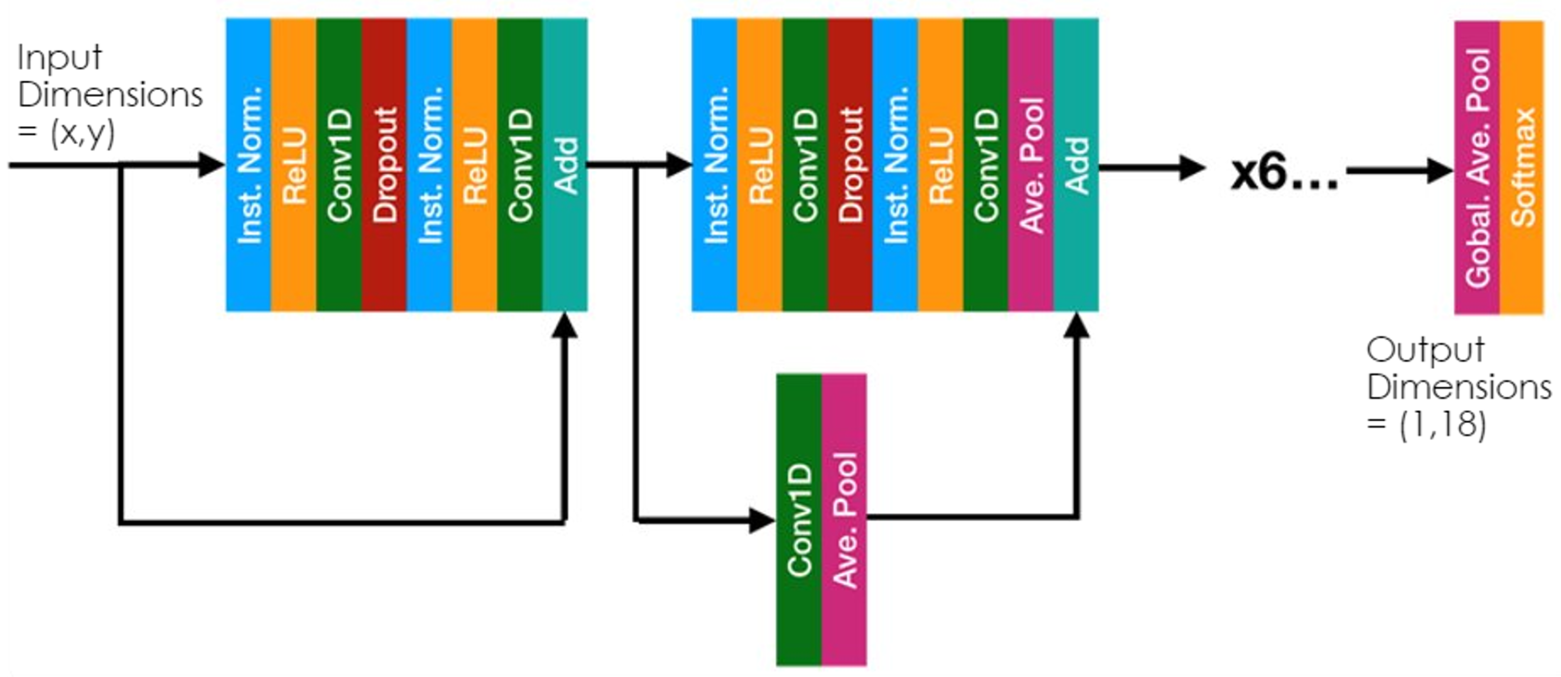
As mentioned previously, the ResNet neural network architecture was used for classification. A diagram of this approach is shown in Figure 1. ResNet is a deep learning architecture that uses residual connections in a cascaded network to allow for efficient training of large, deep convolutional networks [8]. Additional fundamentals of deep learning can be found in research from LeCun et al. [9]. Various layers in the ResNet architecture give a variety of benefits to this application. For instance, the convolutional layers provide a translational invariance to the classification process, which allows the features of interest to drift in the domain in which they are processed without classification performance degrading. The translational invariance is valuable for UCE data obtained via NILM because many of the devices (especially COTS devices) are stable in their operation only to within some commercially acceptable tolerance and are likely to drift in their characteristics over time (this is especially evident for UCE characteristics in the frequency domain position, which became of particular interest in this investigation).

In these deep learning architectures, features are not chosen by the programmer. The features are learned by the neural network based upon the nature of the input and the structure of its architecture. Certain aspects of a feature may be seen by examining the input and output of each layer of the network. Some tools and methods allow a certain level of explainability; development of these methods has mainly focused on imaging applications such as image classification. Examples of the types of methods include DeepLIFT [10] and Integrated Gradients [11], which assume differentiability of the model and propagate the prediction to features using gradients. Perturbation-based methods, such as LIME [12], are also available. LIME is applied to a subset of the devices in this dataset in [13] via formation of a spectrogram with FFT and subsequent analysis. The methods utilized in [13] are validated for this application by human inspection of the very clean and undisturbed data set that was collected. The methods described in this paper could be loosely grouped into the perturbation-based methods approach for explainability.

Understanding the details of the features important to the ResNet model when using a complicated and obscured data set described in the prior section is challenging. Certain levels of understanding can be drawn regarding the features of most value and the effects of noise on the classification performance of the ResNet model by using a methodical process of data augmentation and experimentation to infer something about what the model is doing.

A few variations in the training process and validation sets were used, and these are described in detail in Section 3.1.

2.3. UCE Preprocessing Techniques

Variations of preprocessing methods investigated in this work include “no preprocessing”, FFTs, variations in the length of the FFT, and variations in the window function applied to the raw time-domain data samples prior to applying an FFT.

2.3.1. No Preprocessing

“No preprocessing” involves passing the raw time series data directly into the ResNet classification network. If features were more easily seen in the time domain, the no-preprocessing technique would yield superior results. This technique was applied with some success by He and Chai [6]. Here, the authors include the case of using the ResNet to classify the raw time domain samples, which establishes a baseline performance with which to compare the various preprocessing techniques.

2.3.2. Fourier Transform

“FFT”, if not otherwise specified in this paper, refers to the magnitude calculation of a basic Fourier transform operation performed with a rectangular/uniform windowing function $w\left(n\right)$ applied, where $w\left(n\right)$ is described by Equation (3),

$$w\left(n\right)=1,0\le n\le N$$

(3)

where N is the length of the FFT computation.

2.3.3. Magnitude vs. Complex FFT

When computing the FFT, the previous efforts for classification of equipment with UCE mentioned in Section 2.1 used the magnitude FFT computation. One question is whether including phase will improve the classification. If phase is an important feature of the data, either complex FFT data or time domain data are required. In the NILM-acquired UCE classification applications, the value of the phase of the data are yet unknown. In research from O’Shea et al. [14], some experiments were conducted with classification of communications signals, for which phase information is a feature of high value. In research from Virtue et al. [15], neural networks with complex activation functions have been used in magnetic resonance imaging fingerprinting. In some cases, the real and imaginary components are sent into the deep network as two-dimensional floating point values, as in research from Wang et al. [16]. Here, the authors performed a test with this approach of inputting the real and imaginary components separately into the ResNet with no modification to the ResNet to perform complex math. Results were poor and are not included in Section 3. Efforts are planned to incorporate complex math into the network.

2.3.4. FFT Window Length

A thorough description of the FFT and the concept of windowing time-domain signals can be found in a book by Schafer and Oppenheim [17]. An example equation of window application is shown in Equation (4).

$$y\left(n\right)=x\left(n\right)w\left(n\right),0\le n\le (N-1),$$

(4)

where $x\left(n\right)$ represents the time-domain samples being windowed and $w\left(n\right)$ represents the windowing coefficients being applied. This window application is performed over a finite interval length N. Since increasing N results in higher resolution in the frequency domain, one set of experiments varying N was performed to determine the effects of the additional spectral resolution. Increasing spectral resolution should improve classification results until the resolution exceeds the spectral width of the features determined by the classifier. The noise floor also drops about 3 dB for each doubling of the value of N. On the down side, larger values of N results in lower resolution in the time-domain. Therefore, an important assumption in this trade-space evaluation and feature hypothesis generation (limited explainability attempt for the ResNet classifier) is the assumption that N will not be chosen to exceed the short-term stationarity of the features and noise being used for classification of the devices. A rectangular uniform window was used for the window length experiment. The amount of data used for training, validation and testing was the same regardless of the window length used (smaller window lengths produced more machine learning samples).

2.3.5. FFT Window Type

Nonuniform windows are used to compensate for the facts that N is not infinite and the window is not an integral number of cycles of each of the frequency components in a given segment of data. The question of which window type to apply can be determined a priori if both spectral characteristics of the noise and features used for classification are known. However, this is always difficult or impossible to know in NILM-obtained UCE data collections. In many applications, a Hanning window or other similar window can be used to strike a balance in the spectral resolution and spectral leakage trade space. The authors have introduced a method of determining important features of the signal and noise by sweeping the window type and looking at the classification success. Additional background information to help in understanding the interpretation of the results of this work can be found in [17].

In this application, the authors control the noise generated and can partially anticipate the effect that it might have on the classification. Therefore, because the window type is swept across a continuum of characteristics and noise levels and can monitor the classification accuracy for each trial, the authors can better hypothesize what features of the data set (of a subset of features) are most important. In addition, this allows the authors to hypothesize concerning the effectiveness of the system, given the addition of other types of noise to the data set being studied.

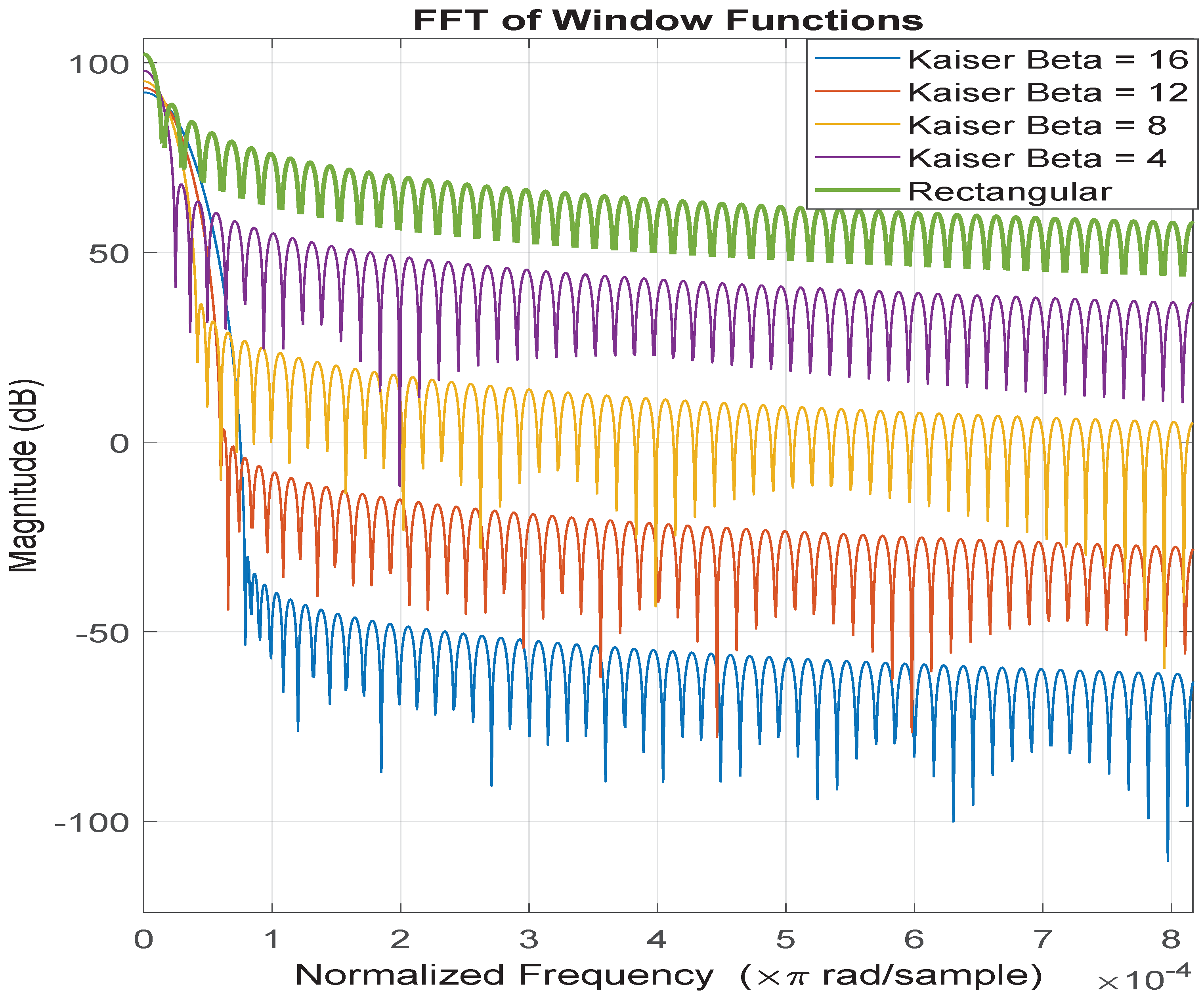
The five window types used in this comparison are rectangular/uniform and Kaiser $\beta =4,8,12,16$. The FFT of each of the window functions is given in Figure 2.

Because multiplication in the time domain is equivalent to convolution in the frequency domain, the spectral domain plots of the windows provide a view of what is happening to the signal in the frequency domain as it is windowed. Windows with more spectrally narrow main lobes will have better spectral resolution and those with the lowest sidebands will have the best spectral leakage suppression. These key characteristics of the five window types are described in

Table 2. Listing of key window function characteristics.

Window	Sidelobe Attenuation (dB)	Mainlobe Width ($-3$ dB)
Kaiser $\beta$ = 16	$-122.4$	3.2325 × 10${}^{-5}$
Kaiser $\beta$ = 12	$-90$	2.861 × 10${}^{-5}$
Kaiser $\beta$ = 8	$-58.7$	2.2888 × 10${}^{-5}$
Kaiser $\beta$ = 4	$-30$	1.7166 × 10${}^{-5}$
Rectangular	$-13.3$	1.3351 × 10${}^{-5}$

.

As the main lobe of the window spectrum is widened, the sidelobe attenuation increases and leakage factor decreases. As the mainlobe width is narrowed, the window achieves a higher level of spectral resolution. This is the main basic trade-off in window selection. The goal in the authors’ selection of these window types was to relatively evenly space the windows in the trade space and observe the differential in classification performance, which would make it easier to draw inferences regarding features used by the ResNet.

2.3.6. Other Modern Spectral Estimation Techniques

One last notable set of methods of preprocessing is that of other spectral estimation techniques, such as autoregressive, moving average, or autoregressive moving average techniques. These techniques are described by Kay [18] and would apply in cases with short data segments. The authors validated that the segments were long enough such that this was not a limitation for the FFT preprocessing spectral estimator. Therefore, no additional investigation of other spectral estimation methods was pursued or planned.

3. Results

In this section, results are presented comparing Time and Frequency domain for classification, evaluating the impact of window length on classification, and studying the impact of window type on classification.

3.1. Time vs. Frequency Domain Preprocessing

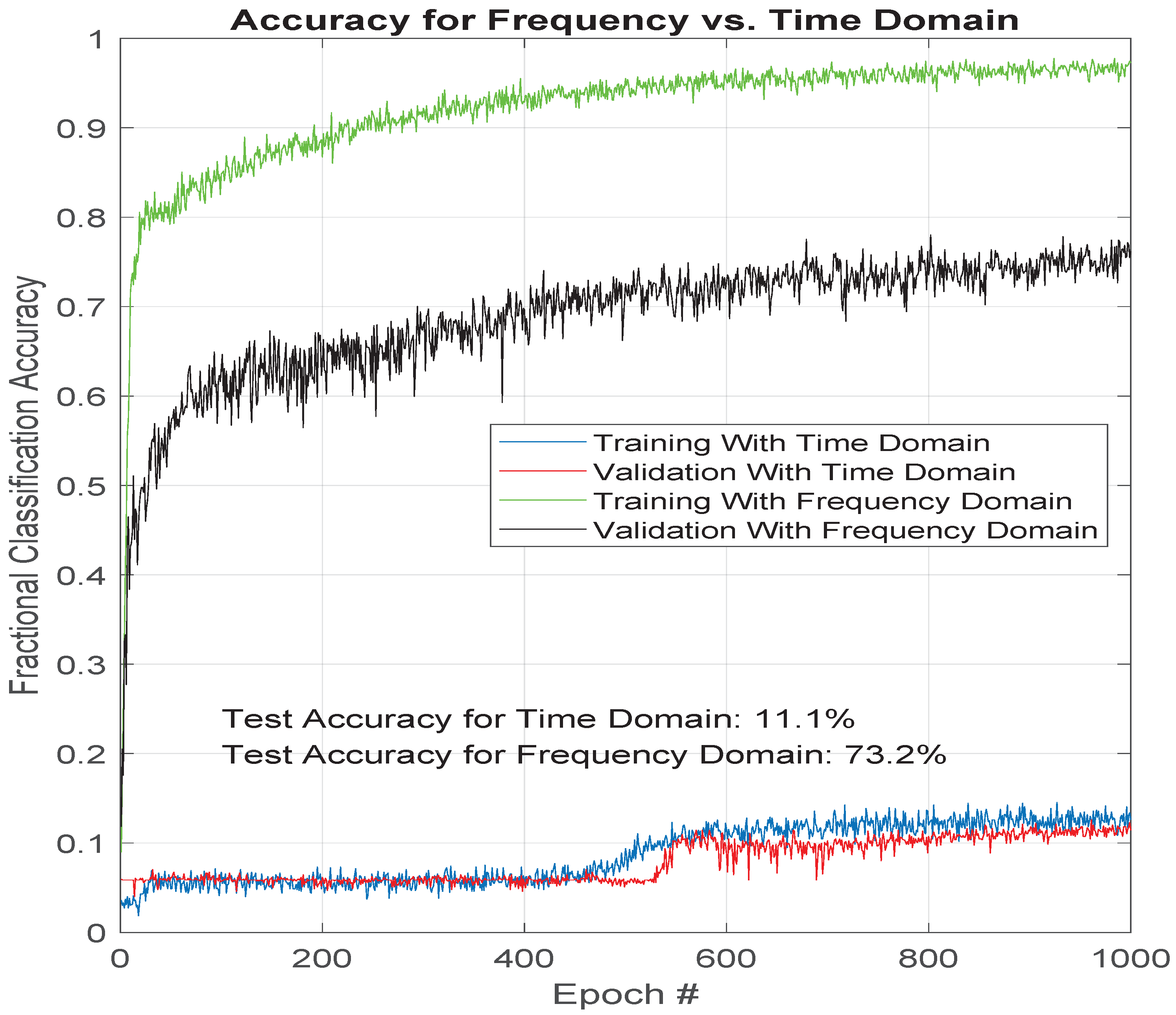
With knowledge that electrical equipment produces features in the frequency domain and the prior successful application of frequency-based signal processing techniques with the linear discriminant analysis classifier given by Vann et al. ([3,5]), the first experiment performed was a comparison of classification in the frequency domain versus the time domain. Results from this comparison verified that the ResNet-based classifier trained and tested with frequency domain data trained quicker and provided higher accuracy than the time domain.

To determine a baseline on the frequency domain classification attempt, the authors performed a simple rectangular windowing prior to the FFT. One way to view the difference in training time and classification performance is shown in Figure 3, which shows the validation classification accuracy as a fraction vs. the training epoch. It demonstrates faster convergence during the training process, as well as a higher performance level in the end (75% accuracy for frequency domain and 11% accuracy for time domain).

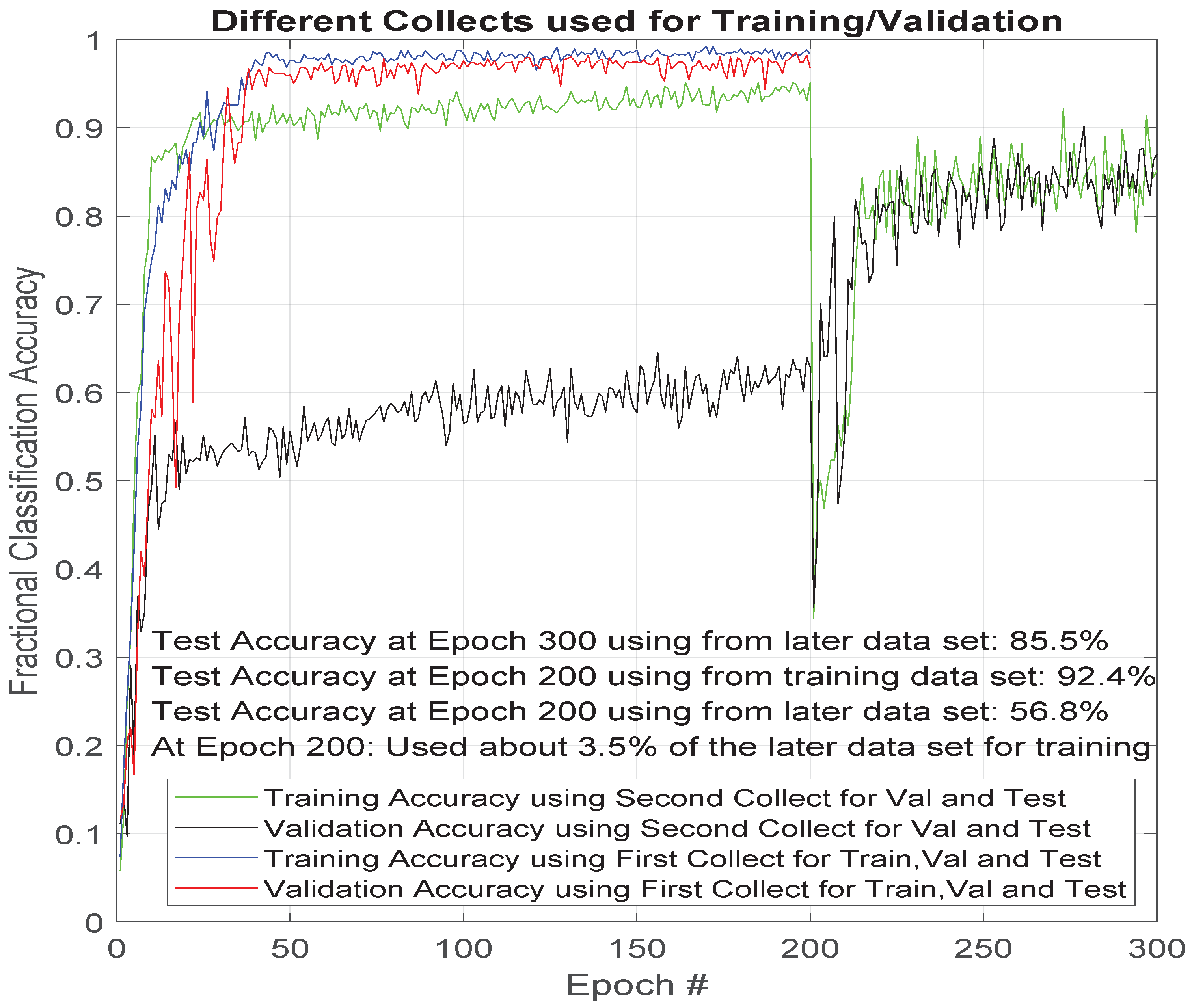
As mentioned earlier, each device in the data set used in this effort were measured for two 10 min periods separated in time. During this effort, the authors observed a significant drop in accuracy that when testing on one of these two collections and training on the other. This drop is a result of the devices or background noise changing between the two collection period. Their features of interest to the classifier were stationary during a single collect period but not between the collection periods. This drop can be most easily seen in Figure 4. This figure shows about 30% worse classification performance for the case in which the training and validation sets were split across time.

At epoch 200, the authors began training the ResNet classifier with a very small set of data from the second collection period, which substantially helped the performance of the validation and test of the classifier as measured by the classification accuracy. The amount of data used in the training was only approximately 1 out of 30 of the available data segments from the second collection for each device.

This experiment implies two principles for this application:

• Training data must fully represent the variability over time in the UCE signals. Otherwise, a good representation of the breadth of characteristics for each device will not be learned by the ResNet classifier.
• Retraining can improve performance. This example showed the potential to improve classification with continued training on small amounts of additional data in time.

Additionally, more complex data augmentation methods may be useful in diverting the classifier from focusing on time-dependent features.

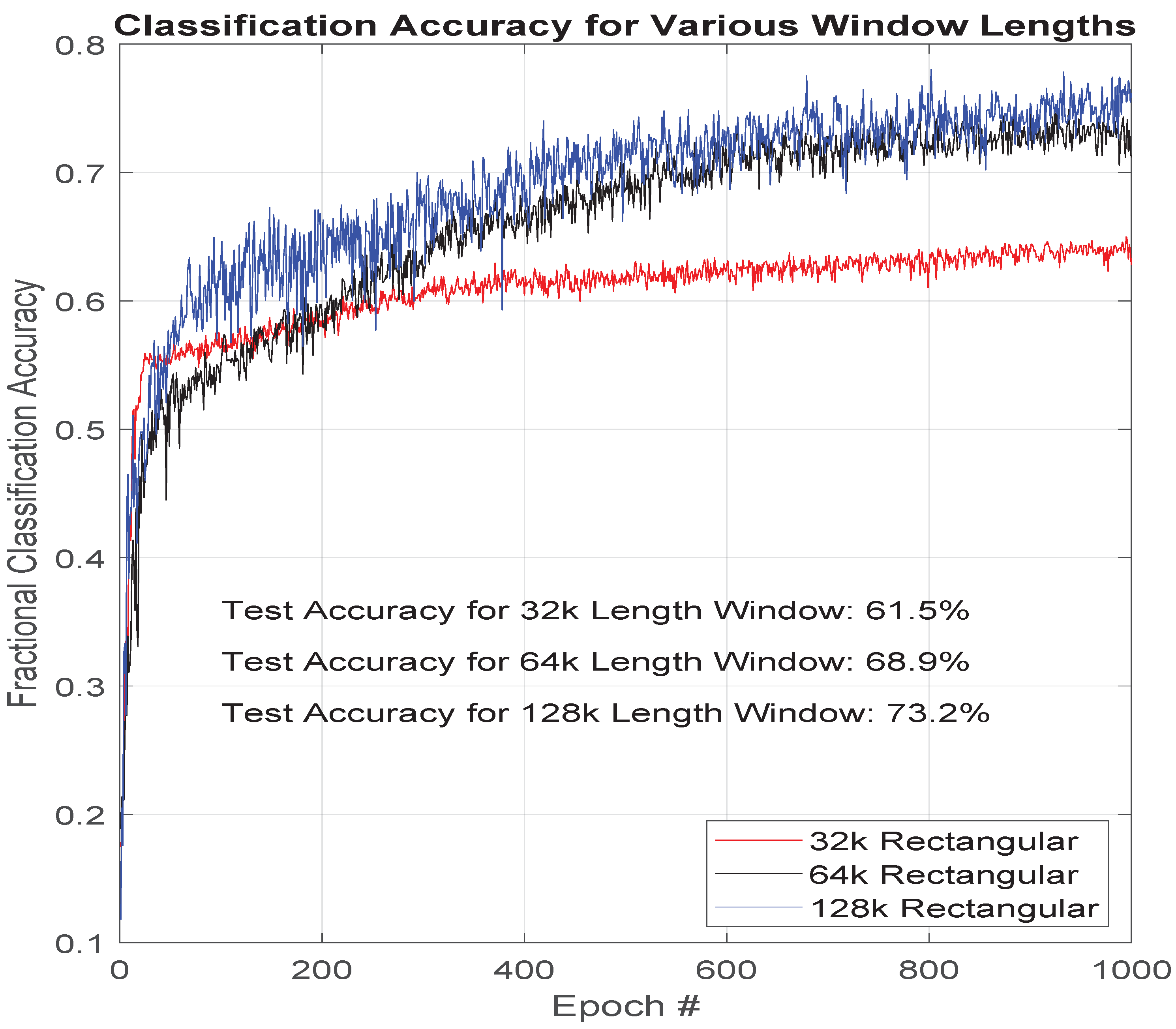
3.2. FFT Window Length

Another preprocessing parameter that was evaluated is the length of the computation of the FFT window. Increasing the length of the FFT results in a resolution increase in the frequency domain. The authors found that increased spectral resolution had a positive effect on classification performance, but the return diminished as spectral resolution increased as shown in Figure 5. The gain of the enhancement of the spectral resolution, which is calculated as given in Equation (5) given the main lobe width of $0.1\times {10}^{-4}$ rad and sample rate of $2\times {10}^6$ Hz, ceased to be of as much value relative to the loss in time resolution. Assuming the window length to be within the stationary period of the augmented data, which is likely given prior testing and results, the combination of Figure 5 and Equation (5) indicates that the features of interest to our deep classifier are not any closer than 3 Hz to one another, and not much narrower than 3 Hz in bandwidth.

$$\frac{(0.1\times {10}^{-4}\mathrm{rad})(2\times {10}^6\mathrm{Hz})}{2\pi \mathrm{rad}}=3\mathrm{Hz}$$

(5)

An alternative and possibly complimentary explanation is that the increasing of the window length, which has the additional effect of lowering the noise floor, reaches a point at which it has uncovered all the easy-to-uncover spectral attributes from the noise floor and the remainder of distinguishable features are buried further down into the noise floor. In future work we plan to determine with more specificity to what degree each of the two factors (spectral resolution increase explanation vs. noise floor decrease explanation) was to credit for the diminishing improvements by running additional experiments with additional levels of noise augmentation. This would then inform us more specifically regarding the features used by the deep classifier.

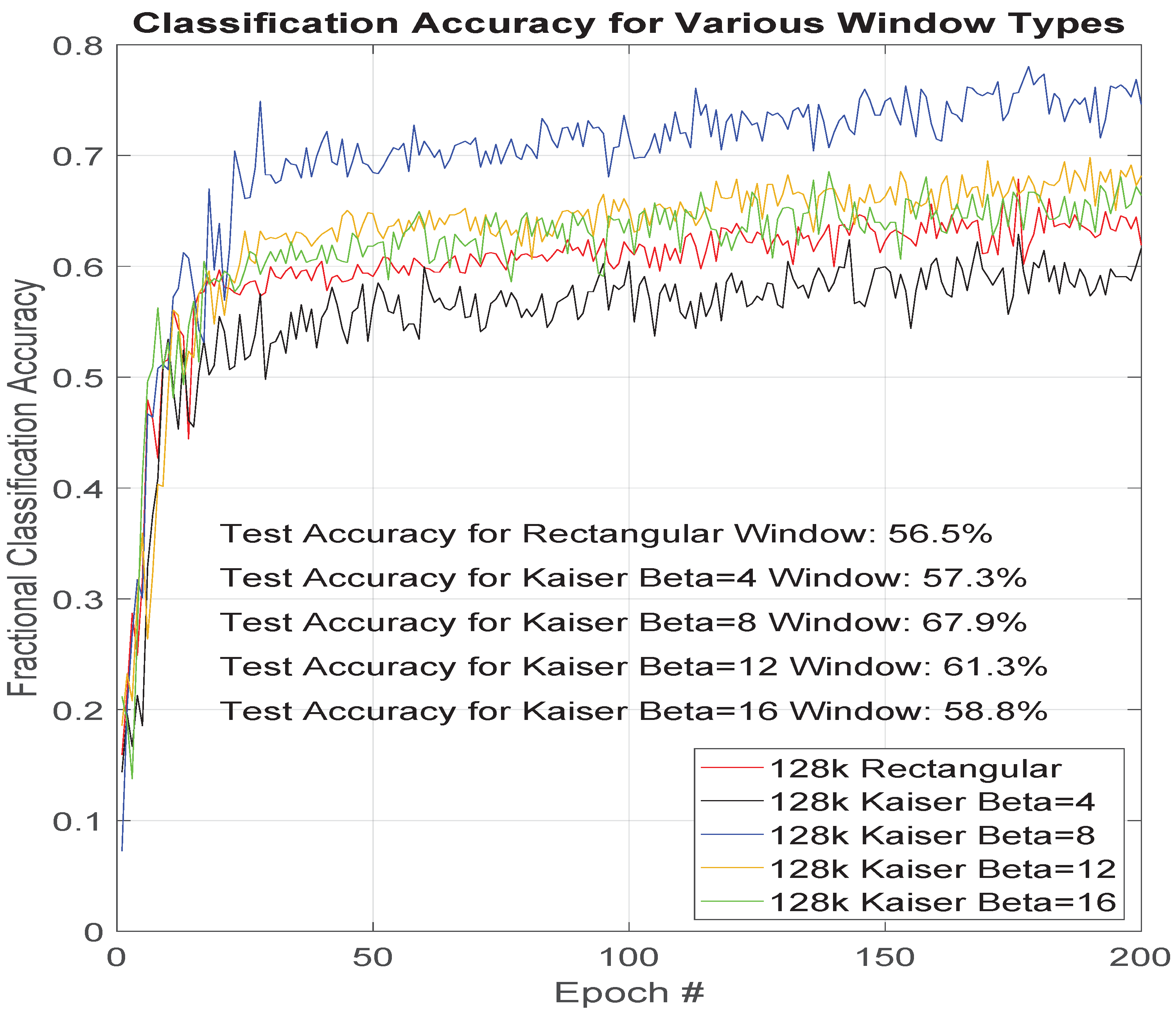
3.3. FFT Window Type

Another experiment performed was a variation of the window type. The differences in the frequency domain of the windows used in this investigation were discussed in Section 2.3.5 and are shown in Figure 2.

Figure 6 shows classification results as a function of training epochs for five different FFT window types. Knowing the attributes of the tested window types and the performances recorded in Figure 6, provide additional understanding of features of the data set are most important to the ResNet classifier.

Resolving features of a particular collection that are close in frequency necessitates a smoothing window with a maximally narrow main lobe in the frequency characteristic. The authors saw the rectangular window perform poorly, as shown in Figure 6. However, they also saw that the other extreme in the trade space (Kaiser $\beta =16$) was approximately equally poor in performance. The optimal window type for this window family of shapes would be somewhere between Kaiser $\beta =8$ and Kaiser $\beta =12$ but closer to the $\beta =8$ case because of its 6.6% better performance. The 95% confidence intervals for the percentages given in Figure 6 are given in

Table 3. Listing of Key Window Function Characteristics.

Window	Classification Accuracy %	Confidence Interval %
Kaiser $\beta$ = 16	58.8	$\pm 1.67$
Kaiser $\beta$ = 12	61.3	$\pm 1.65$
Kaiser $\beta$ = 8	67.9	$\pm 1.57$
Kaiser $\beta$ = 4	57.3	$\pm 1.67$
Rectangular	56.5	$\pm 1.67$

.

The ability to resolve spectral components (either to isolate a feature from noise or separate between two features of two devices) appears to be valuable within some level but must be balanced with the need to reject noise far from the features of interest and prevent the spectral leakage that occurs in the finite-length FFT calculation. It also must be balanced with the possible need to preserve the associated spectral amplitude accuracy. The window function application provides a certain amount of processing gain for certain features. Although the window-type experimental results follow an understandable pattern, they do not point to a specific window that would be optimal but instead to certain window characteristics that are more favorable and then inherently to the types of features being favored by the deep ResNet classifier.

4. Discussion

For the particular data set studied, these results show that a ResNet classifier works best in the frequency domain with a 128K wide Kaiser $\beta =8$ window. However, these results are highly dependent on the characteristics of the signals being classified, noise characteristics present in the collections, the quality and amount of data for training, and the type of deep network. One school of thought is that there is no need to preprocess data for a deep network as it will learn the features of interest. A deep neural network could learn an FFT or specific preprocessing technique given enough data, however, the time versus frequency analysis in this effort shows that FFT preprocessing led to a higher accuracy for the amount of data provided for training. If there are limits in the data collection to short time periods or if the signals being classified change in time such that higher time resolution is required, then a shorter window may be needed. If the spectral bandwidth of UCE features from items to be classified varies significantly from the items in this data set, the optimal window type varies.

The results presented in this paper show the value that signal processing techniques provide to preprocessed data for classificaton using a deep neural network. A great difference exists between helpful preprocessing and optimal preprocessing.

This research has many possible directions of future work to improve classification performance, as can be seen in the window type and window length test results. A longer FFT analysis window would have likely produced a better result. However, we understand the trend of diminishing returns and know that we lose time-domain resolution as we increase the FFT window length. Therefore, we simply noted the improvements and trend. Additionally, the best of the window types (Kaiser $\beta =8$) were not exactly in the optimal place, as can be seen from the other results (Kaiser $\beta =4$ and $\beta =12$). The different levels of improvement made for the various chosen techniques were relatively large.

Tests showed that the deep learning architecture of the ResNet accurately classified the set of 18 relatively low-power devices, based upon the UCE even in low FNR situations. Even though complete explainability of reasons for results is currently relatively limited in such deep networks, the authors demonstrated that methodical data augmentation techniques can be used with a spectrum of preprocessing techniques to hypothesize what features and noise are of most significance to the deep learning network. This ability to hypothesize features used by the deep classifier can provide some measure of predictability of performance in a variety of untested scenarios via extrapolation of results and expert-based analysis.

The results here demonstrated that the spectral content was of most importance to the ResNet and that a transformation to the frequency domain combined with good window choices resulted in improved performance in the presence of strong AWGN. The application of a window acted as a filter and provided a certain amount of processing gain and increase of the FNR. The amount of processing gain varied from window to window and was seen directly in a proportional manner as the window properties changed in the ResNet classification results. Training time decreased when better preprocessing was performed.

Additionally, based on results, the authors conclude that the preprocessing gains produced diminishing returns (measured in terms of the ResNet classification accuracy) as the FFT window size increased. The authors’ conclusion regarding this effect is as follows:

1.

The bin size started becoming as narrow as the features being used by the ResNet, and more narrow than is necessary to distinguish any of the spectral features when compared from device to device.

2.

The FFT processing gain lowered the noise floor beyond all of the features easier to find near the floor.

Future investigations may include using the complex output of spectral transforms via complex neural networks and an investigation of the classification importance of phase in NILM-obtained UCE data. More potential future work is to use a genetic algorithm or other such algorithm for selecting alternative parameters for preprocessing. Another couple of interesting investigations are the inclusion of noise augmentation methods and consideration of time-varying electronic signatures instead of steady-state.

References

- Paul, C.R. Introduction to Electromagnetic Compatibility; John Wiley & Sons: Hoboken, NJ, USA, 2006; Volume 184. [Google Scholar]
- Nassar, M.; Lin, J.; Mortazavi, Y.; Dabak, A.; Kim, I.H.; Evans, B.L. Local utility power line communications in the 3–500 kHz band: Channel impairments, noise, and standards. IEEE Signal Process. Mag. 2012, 29, 116–127. [Google Scholar] [CrossRef]
- Vann, J.M.; Karnowski, T.P.; Kerekes, R.; Cooke, C.D.; Anderson, A.L. A dimensionally aligned signal projection for classification of unintended radiated emissions. IEEE Trans. Electromagn. Compat. 2017, 60, 122–131. [Google Scholar] [CrossRef]
- Hart, G.W. Nonintrusive appliance load monitoring. Proc. IEEE 1992, 80, 1870–1891. [Google Scholar] [CrossRef]
- Vann, J.M.; Karnowski, T.; Anderson, A.L. Classification of Unintended Radiated Emissions in a Multi-Device Environment. IEEE Trans. Smart Grid 2018, 10, 5506–5513. [Google Scholar] [CrossRef]
- He, W.; Chai, Y. An Empirical Study on Energy Disaggregation via Deep Learning. Adv. Intell. Syst. Res. 2016, 133, 338–342. [Google Scholar]
- Cooke, C.D.; Reed, F.K.; Prince, L.J.; Vann, J.M.; Anderson, A.L. An efficient sparse FFT algorithm with application to signal source separation and 2D virtual image feature extraction. In Proceedings of the MILCOM 2016-2016 IEEE Military Communications Conference, Baltimore, MD, USA, 1–3 November 2016; pp. 396–400. [Google Scholar]
- He, K.; Zhang, X.; Ren, S.; Sun, J. Deep residual learning for image recognition. In Proceedings of the IEEE Cconference on Computer Vision and Pattern Recognition, Las Vegas, NV, USA, 27–30 June 2016; pp. 770–778. [Google Scholar]
- LeCun, Y.; Bengio, Y.; Hinton, G. Deep learning. Nature 2015, 521, 436. [Google Scholar] [CrossRef] [PubMed]
- Shrikumar, A.; Greenside, P.; Kundaje, A. Learning important features through propagating activation differences. In Proceedings of the 34th International Conference on Machine Learning, Sydney, Australia, 6–11 August 2017; Volume 70, pp. 3145–3153. [Google Scholar]
- Sundararajan, M.; Taly, A.; Yan, Q. Axiomatic attribution for deep networks. In Proceedings of the 34th International Conference on Machine Learning, Sydney, Australia, 6–11 August 2017; Volume 70, pp. 3319–3328. [Google Scholar]
- Ribeiro, M.T.; Singh, S.; Guestrin, C. “Why should I trust you?”: Explaining the predictions of any classifier. In Proceedings of the 22nd ACM SIGKDD International Conference on Knowledge Discovery and Data Mining, San Francisco, CA, USA, 13–17 August 2016; pp. 1135–1144. [Google Scholar]
- Grimes, T.; Church, E.; Pitts, W.; Wood, L. Explanation of Unintended Radiated Emission Classification via LIME. arXiv 2020, arXiv:2009.02418. [Google Scholar]
- O’Shea, T.J.; Roy, T.; Clancy, T.C. Over-the-air deep learning based radio signal classification. IEEE J. Sel. Top. Signal Process. 2018, 12, 168–179. [Google Scholar] [CrossRef] [Green Version]
- Virtue, P.; Stella, X.Y.; Lustig, M. Better than real: Complex-valued neural nets for MRI fingerprinting. In Proceedings of the 2017 IEEE International Conference on Image Processing (ICIP), Beijing, China, 17–20 September 2017; pp. 3953–3957. [Google Scholar]
- Wang, Y.; Liu, M.; Yang, J.; Gui, G. Data-driven deep learning for automatic modulation recognition in cognitive radios. IEEE Trans. Veh. Technol. 2019, 68, 4074–4077. [Google Scholar] [CrossRef]
- Schafer, R.W.; Oppenheim, A.V. Discrete-Time Signal Processing; Prentice Hall: Englewood Cliffs, NJ, USA, 1989. [Google Scholar]
- Kay, S. Modern Spectral Estimation: Theory and Application; Pearson Education: Englewood Cliffs, NJ, USA, 1999. [Google Scholar]