An All-Batch Loss for Constructing Prediction Intervals

Abstract

The prediction interval (PI) is an important research topic in reliability analyses and decision support systems. Data size and computation costs are two of the issues which may hamper the construction of PIs. This paper proposes an all-batch (AB) loss function for constructing high quality PIs. Taking the full advantage of the likelihood principle, the proposed loss makes it possible to train PI generation models using the gradient descent (GD) method for both small and large batches of samples. With the structure of dual feedforward neural networks (FNNs), a high-quality PI generation framework is introduced, which can be adapted to a variety of problems including regression analysis. Numerical experiments were conducted on the benchmark datasets; the results show that higher-quality PIs were achieved using the proposed scheme. Its reliability and stability were also verified in comparison with various state-of-the-art PI construction methods.

1. Introduction

The prediction interval (PI) is widely used to evaluate uncertainty. Different from the confidence interval (CI) which only relies on statistical analyses of the observed data, the PI describes the uncertainty by means of predictions, which cover estimates of both model uncertainty and data uncertainty [1]. The PI is thus more reliable and effective than the CI. Compared with the regular point prediction, the PI offers more robust results for follow-up operations with full consideration of prediction uncertainty. The risk of over-fitting problems can also be reduced by the PI, which is beneficial for real-world tasks. PIs have found many successful applications such as wind power generation [2,3,4], water consumption forecasts [5], sinter ore burn-through point forecasts [6], parking demand predictions [7], isolated microgrid systems [8], etc.

In recent years, as statistical learning theory has evolved, feedforward neural networks (FNNs) have become universal approximators which are well suited for approximating nonlinear mappings [9]. However, commonly used point predictions generated by FNNs suffer from the inability to estimate uncertainty. Although plenty of models have been proposed to construct PIs through FNNs and have achieved remarkable results, many of them may be unsuitable for real-world tasks due to high computational costs and complex assumptions. Consequently, new techniques are necessary to efficiently generate high-quality PIs. Existing methods can be classified into two categories: (1) Those that construct PIs indirectly by point estimates based on statistical theory; and (2) those that directly estimate the lower and upper boundaries of PIs.

On the basis of CIs, traditional PI construction methods tend to gain PIs through statistical relationships between point estimates and bias estimates. Chryssolouris et al. [10] and Hwang and Ding [11] developed the Delta method for PI construction based on nonlinear regression by applying asymptotic theories and employing the NN as a nonlinear regression model. Bishop [12] and MacKay [13] utilized the Bayesian technique to construct PIs. Due to the introduction of the Hessian matrix, this method suffers from the burden of high computational complexity. Heskes [14], Carney et al. [15] and Errouissi et al. [16] adopted the bootstrap method to construct PIs with FNNs. Bootstrap procedures are useful for uncertainty estimates, and are widely used in many fields, as they provide reliable solutions to obtain the predictive distribution of the output variables in NNs [17]. It has been shown that while the bootstrap method generates more reliable PIs than other methods [18], it suffers from high computational costs under large datasets.

A special case of a traditional PI construction method is the mean-variance estimation (MVE) method, proposed by Nix and Weigend [19]. The MVE method has a low computational cost and is easy to implement because of the dual-FNN structure. However, due to the assumption that the error term obeys a normal distribution with the expectation of the true target, this method may yield bad results in real-world datasets.

In order to reduce computational complexity, Khosravi et al. [20] developed the lower upper bound estimation (LUBE) method to estimate the lower and upper boundaries of PI directly by FNNs. The LUBE method is a distribution-free PI construction method which uses heuristic search algorithms such as Simulated Annealing (SA) [20], Genetic Algorithm (GA) [21] and Particle Swarm Optimization (PSO) [22] to adjust model parameters. Unlike traditional PI construction methods, the LUBE method attempts to improve the quality of PIs instead of focusing on prediction errors. Due to the flexibility of LUBE, it is gaining popularity in several communities, such as solar power prediction [23].

Nevertheless, in the case of large-scale models, the heuristic search scheme adopted by the LUBE method makes it difficult to obtain optimal results. Since gradient descent (GD) has become the standard training method for FNNs [24], it is poorly-suited to production environments.

To introduce the GD into the training process, Pearce et al. [25] proposed the quality-driven (QD) loss method. The QD loss is a differentiable loss function which is based on the likelihood principle, thus rendering the NN-based PIs trainable by GD. In order to reduce the computational cost, the QD loss applies the central limit theorem to approximate the binomial distribution during the derivation, which has the requirement for the minimum amount of data (50 points for example [25]) involved in each calculation epoch. If the minibatch method is used for training, a large batch size should be selected, which may reduce the generalization performance of the model and cause a waste of computing resources [26]. Hence, QD loss is unsuitable for training on small sample sets as it may cause errors due to a lack of data. Thus, the application of QD loss is limited because of the fact that it is difficult to obtain large sample sets in many real-world tasks [27]. However, recently, QD loss has received a lot of attention for its diversion and simplicity.

On the basis of the QD loss method, Salem et al. [28] developed the SNM-QD+ method. By introducing the split normal density (SND) functions and penalty functions, they improved the stability of the training process. However, the method did not solve the problems of poor training reliability in the case of small-batch data and the gradient disappearance during training.

Based on a literature review, the following aspects were found to be lacking:

• Some existing methods are not able to handle large-scale data because of the high computational costs, while other methods are unsatisfactory for small-batch data due to assumptions regarding data distribution. No method that can be applied to all batch sample sizes at present;
• Many of the PI generation methods suffer from a fragile training process. Due to the ubiquitous disadvantage of high computational complexity, existing methods may be more likely to suffer from problems such as over-fitting, gradient disappearance and gradient explosion when encountering complex models;
• It is difficult to get high-quality point estimates and PIs at the same time.

To address the aforementioned problems, this paper proposes an all-batch (AB) loss function to construct high-quality PIs. On the basis of making full use of the advantages of likelihood principles, the proposed AB loss function can be applied to both small and large batches of samples. With the structure of dual FNNs, a PI generation framework is also proposed which can output point estimates and bias estimates to build PIs. The accuracy and flexibility of the proposed method are validated by experiments conducted on ten regression datasets; the results show that the proposed scheme can handle small-batch data. Different from existing methods, the proposed scheme probes the following strategies:

• Instead of using the central limit theorem as the approximator, the AB loss estimates the likelihood function directly by adopting the Taylor formula, which enables the AB loss to adapt to both small and large batches;
• To address the problem of the gradient disappearance which occasionally occurs during the training by QD loss, a penalty term for misclassification is proposed. The proposed penalty term can speed up the convergence of the model and improve the quality of the output PIs;
• By utilizing the structure of the dual FNNs similar to the MVE method, the point estimates and the bias estimates can be obtained separately without affecting each other, which is more flexible in real-world tasks.

The remainder of this paper is organized as follows. Section 2 introduces the AB loss as well as the proposed PI generation framework. Numerical experiments are conducted in Section 3. Section 4 discusses the experimental results and the future work. Finally, Section 5 draws conclusions.

2. Materials and Methods

This section first describes the mathematical concepts of PI, and then introduces the QD loss method. Finally, the AB loss function as well as the PI construction framework with dual-FNN structure are built to generate high-quality PIs.

2.1. Prediction Interval

Since PI can be applied in most regression tasks, regression analysis was chosen as the topic of this paper. In most regression problems, the relationship between input and output can be expressed as:

$$y=f(x)+\epsilon ,$$

(1)

where $x$ and $y$ are the observation values of input and output respectively, $f$ is the input-output mapping operator, which refers to the training model and $\epsilon$ is the noise with zero expectation.

To simplify the problem, we assume that the errors are independent and identically distributed (i.i.d.). Then, the variance of the problem can be expressed as:

$${\sigma }^2={\sigma }_{\omega }^2+{\sigma }_{\epsilon }^2,$$

(2)

where ${\sigma }_{\omega }^2$ refers to the model misspecification and parameter estimation variance, and ${\sigma }_{\epsilon }^2$ refers to the noise variance in observation data [29]. The main target of PI is to estimate these deviations in the form of upper and lower boundaries.

As described in the LUBE method [20], confidence and sharpness are two aspects for quality evaluation of PIs. Quantifying the quality of PIs facilitates the construction of an efficient PI generation model.

2.1.1. Confidence

High-quality PIs should ensure high confidence. In order to quantify the confidence, the confidence level $(1-\alpha )\%$ is defined as the probability that the observation is contained by the upper and lower boundaries of PI. Define vector $\beta$ which represents whether the current point is captured by PI formally.

$${\beta }_i=\{\begin{array}{c}1,if{y}_i\in [L_i,U_i],\\ 0,if{y}_i\notin [L_i,U_i],\end{array}$$

(3)

where $y_i$ is the observation value, $L_i$ and $U_i$ represent the lower and upper boundaries of PI. Thus, the total number of observations captured by PIs can be defined as follows:

$$c={\displaystyle {\sum }_{i=1}^n{\beta }_i}.$$

(4)

According to this, PI coverage probability (PICP) demonstrates the probability that target values are captured by PIs.

$$PICP=c/n,$$

(5)

where $n$ represents the total number of the observations. The quality of generated PIs can be estimated by the comparison between PICP and confidence level [20,30,31,32].

2.1.2. Sharpness

In addition, high-quality PIs have requirements for both confidence and sharpness. In most existing methods, sharpness is mainly defined as the distance between the upper and lower boundaries. It is clear that if the distance approaches infinity, the PICP of the PI tends to 100%. Thus, to measure the width of PIs, normalized mean prediction interval width (NMPIW) is defined as follows [20,30,32]:

$$NMPIW=1/(nR){\displaystyle {\sum }_{i=1}^n(U_i-L_i)},$$

(6)

where $R$ is the range of the underlying target, $U_i$ and $L_i$ represent the upper and lower boundaries of PIs corresponding to the $i$th sample. To generate high quality PIs, NMPIW should be reduced as much as possible on the basis of ensuring a certain PICP.

To balance PICP against NMPIW, the coverage width-based criterion (CWC) is defined as follows [20]:

$$\begin{array}{l}\gamma =\{\begin{array}{c}0,PICP\ge \mu \\ 1,PICP\le \mu \end{array},\\ CWC=NMPIW(1+\gamma (PICP)\exp (-\eta (PICP-\mu ))),\end{array}$$

(7)

where $\mu$ is the confidence level and $\eta$ is a hyperparameter determining how much penalty is assigned to PIs with a low coverage probability. Direct PI generation methods like the LUBE method [20] treat CWC as the target function, which enables the model to be trained from the perspective of improving the quality of PIs.

2.2. Quality Driven Loss

As for confidence, the QD loss method takes a likelihood-based approach. Assuming that ${\beta }_i$ is i.i.d. for each index, the total number of observations captured by PIs $c$ obeys a binomial distribution, i.e., $c~Binomial(n,(1-\alpha ))$. According to the central limit theorem, the distribution of $c$ can be approximated by a normal distribution under the condition of a large sample set.

$$Binomial(n,(1-\alpha ))\approx N(n(1-\alpha ),n\alpha (1-\alpha )).$$

(8)

Then, by utilizing the maximum likelihood method, the training goal can be transformed into:

$$\begin{array}{c}-\log L(\theta |\beta ,\alpha )\propto {(n(1-\alpha )-c)}^2/n\alpha (1-\alpha )\\ =(n/\alpha (1-\alpha )){((1-\alpha )-PICP)}^2.\end{array}$$

(9)

As for sharpness, PIs that fail to capture their targets should not be encouraged to shrink further [25]. Therefore, the captured Mean PIs Width (captured MPIW) is proposed as the sharpness measurement.

$$MPI{W}_{capt.}=1/c{\displaystyle {\sum }_{i=1}^n(U_i-L_i){\beta }_i}.$$

(10)

Finally, the QD loss is given as follows:

$$\begin{array}{l}Los{s}_{QD}=MPI{W}_{capt.}+\\ \lambda \frac{n}{\alpha (1-\alpha )}\max {(0,(1-\alpha )-PICP)}^2,\end{array}$$

(11)

where $\lambda$ is a hyperparameter that controls the importance of confidence vs. sharpness.

To solve the problem that PICP is non-differentiable, the soft version of PICP is presented as follows:

$$PIC{P}_{soft}=1/n{\displaystyle {\sum }_{i=1}^n(\sigma ((U_i-y_i)s)\cdot \sigma ((y_i-L_i)s))},$$

(12)

where $\sigma$ is the sigmoid function and $s$ is the softening factor. The QD loss method enables the model to be trained by GD, which greatly reduces the difficulty of implementation, and can be used in large-scale models.

2.3. All-Batch Loss Function

The limitation of the QD loss is the assumption of data scale caused by the use of central limit theorem. In order to improve the quality of PIs in the case of small-batch data, the all-batch (AB) loss function is proposed in this study.

2.3.1. Derivation

Under the assumption of QD loss, the total number of observations captured by PIs $c$, which is defined in (4), can be represented by a binomial distribution, i.e., $c~Binomial(n,(1-\alpha ))$. Then, the likelihood function can be expressed as:

$$L_{\theta }=(\begin{array}{c}n\\ c\end{array}){(1-\alpha )}^c{\alpha }^{n-c}.$$

(13)

To simplify the calculation, instead of using the central limit theorem, the AB loss adopts the Taylor formula for direct approximation. Thus, the negative log likelihood (NLL) of the distribution is:

$$\begin{array}{c}-\log L_{\theta }=-{\displaystyle {\sum }_{i=1}^n\log i}+{\displaystyle {\sum }_{i=1}^{n-c}\log i}+{\displaystyle {\sum }_{i=1}^c\log i}\\ -c\log (1-\alpha )-(n-c)\log \alpha .\end{array}$$

(14)

For simplicity, the Taylor expansion of $\log (1+x)$ is introduced.

$$\log (1+x)={\displaystyle {\sum }_{k=1}^n{(-1)}^k\frac{x^{k+1}}{k+1}}+o(x^{k+1}),x\in (-1,1].$$

(15)

In order to calculate the equation, $x^{\prime }=1+x$ is introduced to transform the equation, and two orders of Taylor expansion are taken for the approximation.

$$\log (x^{\prime })\approx -\frac{1}{2}{x}^{\prime 2}+2x^{\prime }-\frac{3}{2},x^{\prime }\in (0,2].$$

(16)

To meet the requirements of the convergence domain, the NNL is transformed into:

$$\begin{array}{c}-\log L_{\theta }=-{\displaystyle {\sum }_{i=1}^n\log \frac{i}{n}}+{\displaystyle {\sum }_{i=1}^{n-c}\log \frac{i}{n}}+{\displaystyle {\sum }_{i=1}^c\log \frac{i}{n}}\\ -c\log (1-\alpha )-(n-c)\log \alpha .\end{array}$$

(17)

With several common series expansions, the intermediate equation can be obtained as follows:

$$\begin{array}{l}{\displaystyle {\sum }_{i=1}^k\log (\frac{i}{n})}\approx \\ \frac{-18k{n}^2+(12k^2+12k)n-2k^3-3k^2-k}{12n^2}.\end{array}$$

(18)

Finally, the NNL can be calculated by:

$$\begin{array}{c}-\log L_{\theta }\approx (\frac{1}{2}-\frac{2}{3}n)(1-PICP)PICP\\ -nPICP\log \frac{1-\alpha }{\alpha }-n\log \alpha .\end{array}$$

(19)

During the training process, the output upper and lower boundaries should meet the following condition.

$$U_i>y_i>L_i.$$

(20)

However, if FNNs are used as the main model, the division of the upper and lower boundaries output neurons will be achieved by initializing the network parameters, which is unreliable. In the QD loss method, the upper and lower boundaries obtained by the FNNs may thus encounter the following three situations, which may result in gradient disappearance.

$$\{\begin{array}{c}{L}_i>U_i,\\ U_i>L_i>y_i,\\ y_i>U_i>L_i.\end{array}$$

(21)

To resolve the problem of gradient disappearance, a penalty term is hence applied in the AB loss and could be described below formally.

$$P=\frac{1}{n}{\displaystyle {\sum }_{i=1}^n(\exp (\frac{L_i-U_i}{\beta })+\exp (\frac{y_i-U_i}{\beta })+\exp (\frac{L_i-y_i}{\beta }))},$$

(22)

where $\beta$ controls the importance of the penalty term.

As for sharpness, the captured MPIW which is defined as the distance metric of the upper and lower boundaries is used in the AB loss due to its reliability. Because of the non-differentiable character of the original PICP, the soft version of PICP is used in AB loss. Finally, the AB loss is constructed formally:

$$\begin{array}{c}Los{s}_{AB}=MPI{W}_{capt.}\\ +\gamma ((\frac{1}{2}-\frac{2}{3}n)(1-PIC{P}_{soft})PIC{P}_{soft}\\ -nPIC{P}_{soft}\log \frac{1-\alpha }{\alpha }-n\log \alpha )+P,\end{array}$$

(23)

where $\gamma$ controls the importance between confidence and sharpness.

2.3.2. Comparison with QD Loss

Even if the AB loss and the QD loss are derived from the same assumption, there are many differences between the two methods.

The main difference between the two methods is the different approximation methods for binomial distribution. The QD loss method applies the central limit theorem as an approximator, which assumes that the number of sample points is sufficient. Under such assumptions, each batch should have enough data in the training process, which may consume more computing resources. The correctness of the training results is questionable on the small batch of samples. The AB loss, by contrast, adopts the Taylor formula as an approximator, which may make the best use of the advantages of binomial distribution. Since AB loss only utilizes the second-order Taylor expansion formula during derivation, it may introduce numerical errors into the original NNL. However, QD loss approximates the binomial distribution to a normal distribution, which fundamentally changes the original assumption. Thus, AB loss may yield more reasonable results. Mathematically, the proposed method has no limitation on the size of the training set, which expands its potential for application in deep learning.

Due to the introduction of the penalty term, the AB loss is more stable than the QD loss. During the training process, when the PICP is low, the use of the QD loss may cause the problem of gradient disappearance, which may prevent the training from continuing. The penalty term adopted in the AB loss is conducive to guiding the update of network parameters in the direction of improving PICP. Moreover, the penalty term ensures that the network continues training when the PICP is low, which may improve the stability of the training process.

Another benefit of the penalty term in the AB loss is that it simplifies the training process. When adopting the QD loss for training, the output layer should be initialized according to the range of training data, which limits the application of the QD loss. Nevertheless, when using the AB loss for training, there is no need to independently initialize the output layer of the network. The neurons of the output layer only need to be distinguished logically, which simplifies the training process.

2.4. Prediction Interval Generation Framework

In order to get the point estimates and the PIs at the same time, a PI generation framework with the structure of dual FNNs is proposed in this paper. The generation of PIs is separated from the implementation details of the core model in the proposed framework. By changing the structure of the core model, the proposed framework can be applied to different tasks, such as sequence modeling, classification, etc.

2.4.1. Structure

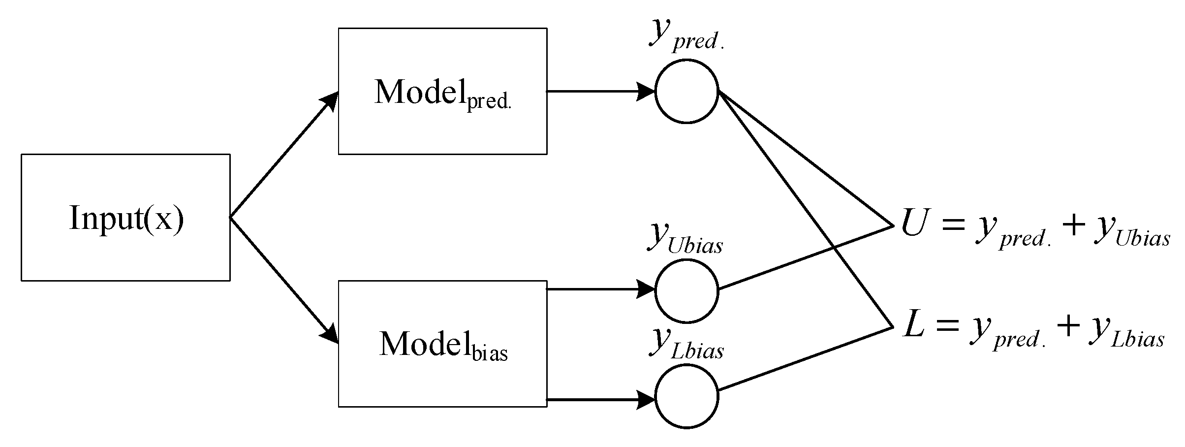
The basic structure of the framework is described in Figure 1. Two FNNs were adopted to generate the prediction estimate and the bias estimate respectively. Consequently, the structure of the prediction model and the bias model could be adjusted separately to meet the requirements of the task.

The selection of the prediction network depends on the type of the task, and the bias network usually utilizes FNNs due to their strong nonlinear approximation ability. In order to make the output of the model consistent regardless of which structure is used, the output format of the two models should be the same.

2.4.2. Framework Training

The loss function of the framework includes two parts: prediction loss and deviation loss. The training process of the framework mainly makes use of the two parts of the loss function to obtain highly reliable PIs with GD. The prediction loss is the loss function adopted to train the prediction network, which needs to be selected according to the task, including L1 loss, Cross-Entropy loss etc. AB loss is chosen to be the main part of the bias loss, and the parameters of the bias network are adjusted by the bias loss to obtain high-quality PIs related to the task.

The training process can be described as follows. Firstly, the preprocessed data is input into the prediction network and the prediction network outputs the prediction estimates. The process can be expressed below:

$$y_{pred.}=f_{M_{pred.}}(x),$$

(24)

where $f_{M_{pred.}}$ represents the model mapping operator of the prediction network, and $x$ refers to the input data and $y_{pred.}$ denotes the predict value.

Then, the preprocessed data is input into the bias network, and the bias network outputs the bias value.

$$y_{bias}=f_{M_{bias}}(x),$$

(25)

where $f_{M_{bias}}$ represents the model mapping operator of the bias network and $y_{bias}$ means the vector contains the upper bias and the lower bias. The upper and lower boundaries can be calculated by the prediction estimate and the bias estimate.

$$\begin{array}{l}L=y_{pred.}+y_{Lbias},\\ U=y_{pred.}+y_{Ubias},\end{array}$$

(26)

where $y_{Lbias}$ and $y_{Ubias}$ are the lower bias and upper bias.

Since GD is the standard method for model training, a GD-based method was adopted for parameter updates. And the final loss of the framework is shown as follows:

$$Loss=Los{s}_{pred.}+Los{s}_{AB},$$

(27)

where $Los{s}_{pred.}$ is the chosen loss function for the prediction model.

3. Experiments

Numerical experiments were conducted to verify the effectiveness and flexibility of the proposed scheme. The data sources include two nonlinear datasets with gaussian noise and exponential noise separately and eight benchmark regression datasets. A comparison among the MVE method, the LUBE method, the QD loss and the AB loss proved that the AB loss with the PI generation framework yielded better results.

3.1. Data Description

Table 1. Dataset used for experiments.

Case Study	Target	Samples	Reference
#1	Nonlinear function with gaussian noise	2000	[25]
#2	Nonlinear function with exponential noise	2000	[25]
#3	Boston housing	506	[33]
#4	Concrete compressive strength	1030	[34]
#5	Energy	768	[35]
#6	Forward kinematics of an 8-link robot arm	8192	[36]
#7	Naval	11,934	[37,38]
#8	Power plant	9568	[39,40]
#9	White wine quality	4898	[41]
#10	Sailing yachts	308	[42]

depicts the details of the used datasets. The datasets denote a number of synthetic and real-world regression case studies from different domains.

In case study 1 and 2, the data are generated from a synthetic mathematical function shown below [25]:

$$0.2\times (1.5\sin (\pi x)+{\sigma }_N),$$

(28)

where $x$ is the input term, and ${\sigma }_N$ is the noise term that subjects the normal distribution, i.e., ${\sigma }_N~N(0,x^4)$, in case study 1, while subjects the exponential distribution, i.e., ${\sigma }_N~\exp (1/x^2)$, in case study 2. In order to generate the dataset, the input term in each case study is set to be randomly sampled from interval [−2,2].

In case study 3, a dataset concerning housing prices in the Boston Massachusetts area was adopted. This dataset is often used to verify the effectiveness of regression analysis methods. The dataset in case study 4 contains eight features, which are applied to build a regression model of concrete compressive strength. Case study 5 aims to exploit 12 different building shapes simulated in Ecotect for energy analysis. By using the simulated posture information of each axis of an 8-link robot arm, case study 6 realizes the forward kinematic analysis of the robot. Case study 7 is a numerical simulation of a naval vessel (Frigate) characterized by a Gas Turbine (GT) propulsion plant. The dataset applied in case study 8 is collected from a Combined Cycle Power Plant over 6 years (2006–2011), which is used to predict the net hourly electrical energy output of the plant. Case study 9 employs 11 features to predict the quality of white wine. The dataset in case study 10 is proposed for prediction of residuary resistance of sailing yachts.

3.2. Experiment Methodology

Experiments were conducted on the comparison of PI generation performance among the MVE method, the LUBE method, the QD loss and the AB loss. In order to ensure the fairness of the experiment, the PI generation framework proposed in Section 2 was used as the basic structure in the implementation of the QD loss and the AB loss. In order to get the best possible results, the PSO method was applied for training in the LUBE method while the GD with the Adam [43] optimizer was adopted in the MVE method, the QD loss and the AB loss. Case study 1 compares the performance of the QD loss and the AB loss in the case of small batches, while case study 2 shows the PI generation performance of the MVE method and the AB loss under different noises. Other benchmark datasets verify the reliability and effectiveness of the AB loss on general regression tasks.

As for metrics, a modified CWC was used for model validation. In the original CWC, it was difficult to achieve an appropriate trade-off between confidence and sharpness; this was resolved by introducing additional hyperparameters in the modified CWC [44].

$$\begin{array}{l}PIARW=\frac{1}{n}{\displaystyle {\sum }_{i=1}^n\frac{U_i-L_i}{y_i}},\\ CWC=(1+{\eta }_{1}PIARW)(1\\ +\gamma (PICP)\exp (-{\eta }_2(PICP-\mu ))),\end{array}$$

(29)

where ${\eta }_1$ and ${\eta }_2$ are two hyperparameters that represent the importance between sharpness and confidence. By adjusting these two hyperparameters, the quality of PIs can be evaluated from different aspects.

In case study 1, due to the specific data distribution, the CIs at the 95% confidence level can be easily obtained. The relationship between the PI Width (PIW), which can be estimated by CIs under ideal conditions, and the input variable in case study 1 is described as the formula below:

$$\mathrm{PIW}=2\times 0.2\times 1.96\times x^2,$$

(30)

where $x$ is the input value.

Therefore, for case study 1, a more reasonable metric is to calculate the Mean Square Error (MSE) between the predicted PIW and the expected PIW, which is described as follows:

$$MS{E}_{PIW}=\frac{1}{n}{\displaystyle {\sum }_1^n{(PI{W}_{pred.i}-PI{W}_{\exp c.i})}^2},$$

(31)

where $PI{W}_{pred.i}$ and $PI{W}_{\exp c.i}$ are the predicted PIW and the expected PIW.

The performance of the AB loss and the QD loss were verified by changing the batch size during training. In order to prove that the AB loss has better performance in small batches, the minibatch method is applied for training, and the batch size is set to 16, 32, 64 and 128 for experiments. In other benchmark datasets, the models were trained using the MVE method, the LUBE method, the QD loss and the AB loss separately. The dataset is divided into training set and test set at a ratio of 7:3, and a batch of 128 sample points is used for training according to the minibatch method.

3.3. Parameters

Table 2. Parameters used in the experiments.

Method	Parameter	Numerical Value
Common	$\alpha$	0.05
	$N_{epoch}$	1000
LUBE	$\eta$	50
	$\mu$	0.95
QD Loss	$\lambda$	15
	$s$	160
AB Loss	$\lambda$	0.03
	$\beta$	1.2

summarizes the parameters adopted in the experiments. The number of hidden layer neurons in each FNN is set to 50, and the expected confidence level of the PIs is set at 95%. Meanwhile, the hyperparameters of the MVE method, the LUBE method, the QD loss and the metric CWC are set according to the original paper [19,20,25,44]. The coefficient of the penalty term $\beta$ is set at 1.2 to ensure that it has a small impact during normal training and a big impact when errors occur. The weight parameter of the AB loss is set to 0.03 according to the results of the numerical experiments in case study 1. In all benchmark experiments, to meet the characteristics of each dataset, the weight parameters of the AB loss and the QD loss is set separately to a value that makes the PICP of the result at least equal to the confidence level, which is 95%.

In the LUBE method, due to the complicated network structure, it is hard to find parameters that meet the requirements of the confidence level by PSO. Therefore, the best result after 1000 rounds of iterative search is adopted as the final result in the implementation of the LUBE method.

3.4. Model Comparisions

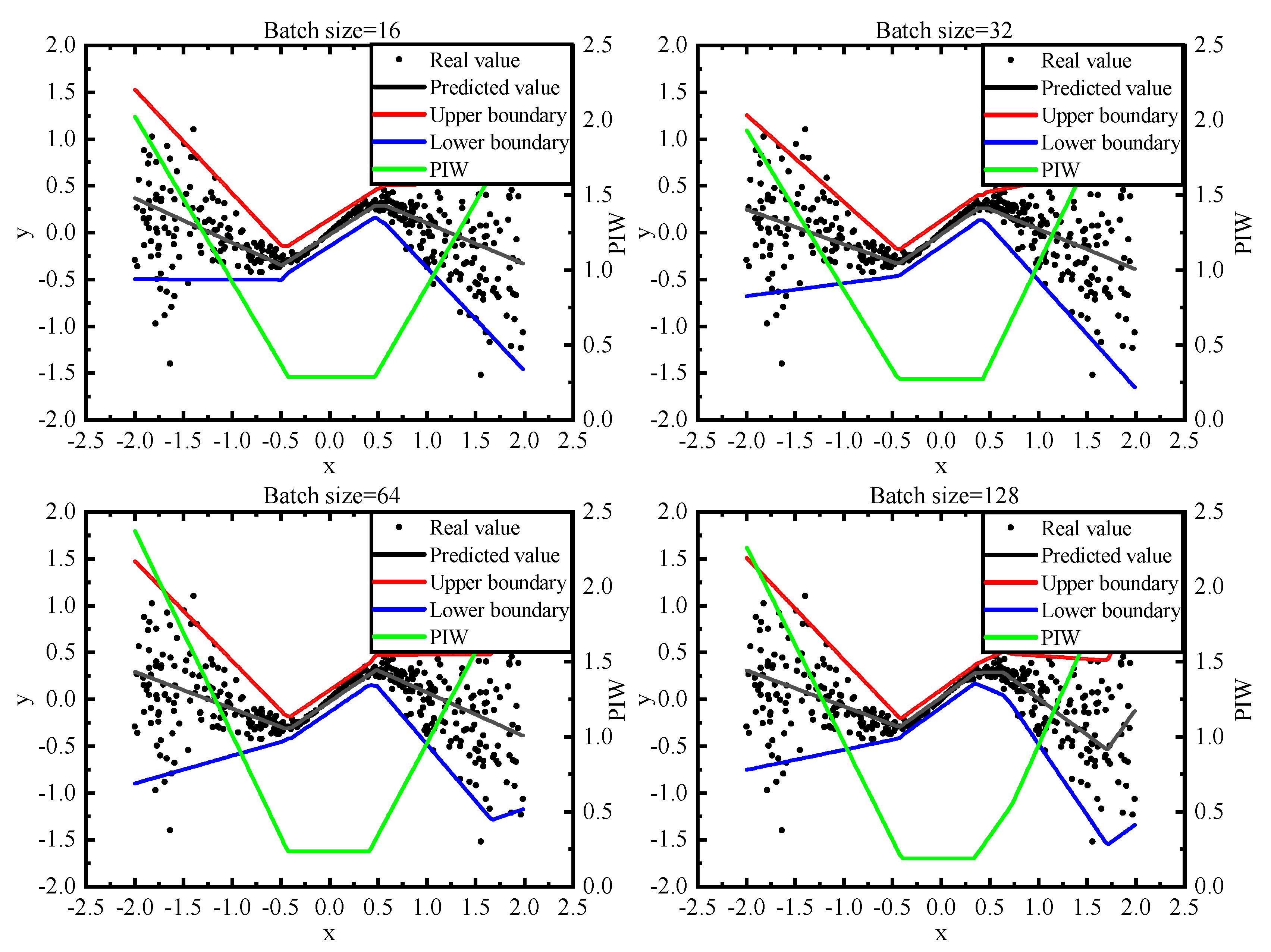
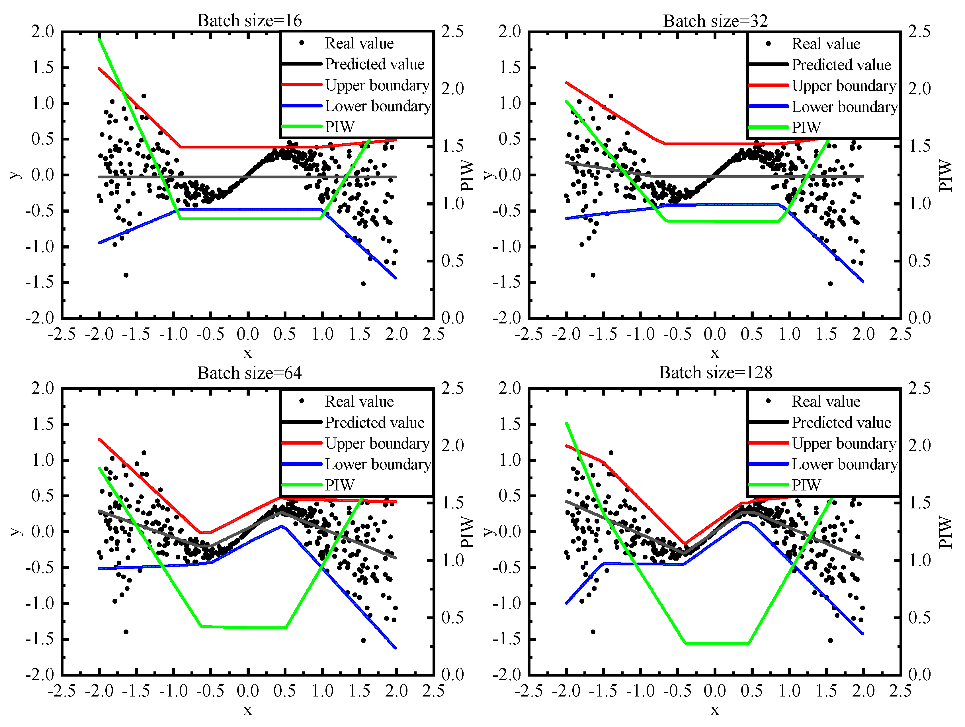
In case study 1, after changing the batch size, the performance of the QD loss and the AB loss is shown in Figure 2 and Figure 3. Compared with the PIs generated by QD loss, the PIs generated by AB loss are closer to the original curve on small batches.

The median values of PICP, MPIW, CWC and MSE metric values of each experiment in case study 1 are shown in

Table 3. Statistical characteristics of PICP, MPIW, CWC and MSE for the QD Loss and the AB loss with changing batch size.

Batch Size	QD Loss				AB Loss
	PICP (%)	MPIW	CWC	MSE	PICP (%)	MPIW	CWC	MSE
16	96.24	1.21	625.40	0.29	95.20	0.94	503.70	0.14
32	96.24	1.17	584.94	0.32	96.74	1.01	515.22	0.13
64	95.49	0.95	488.79	0.20	96.99	1.03	557.50	0.08
128	95.49	0.95	506.38	0.13	97.24	1.02	536.68	0.07

. In the case of small batches, the model trained with AB loss has a significant improvement in MSE. As for the CWC metric, using AB loss has an improvement of up to 20%, which is mainly because of the average situation which is considered by CWC metric. The results prove that the AB loss is more reliable than the QD loss in the case of small batches.

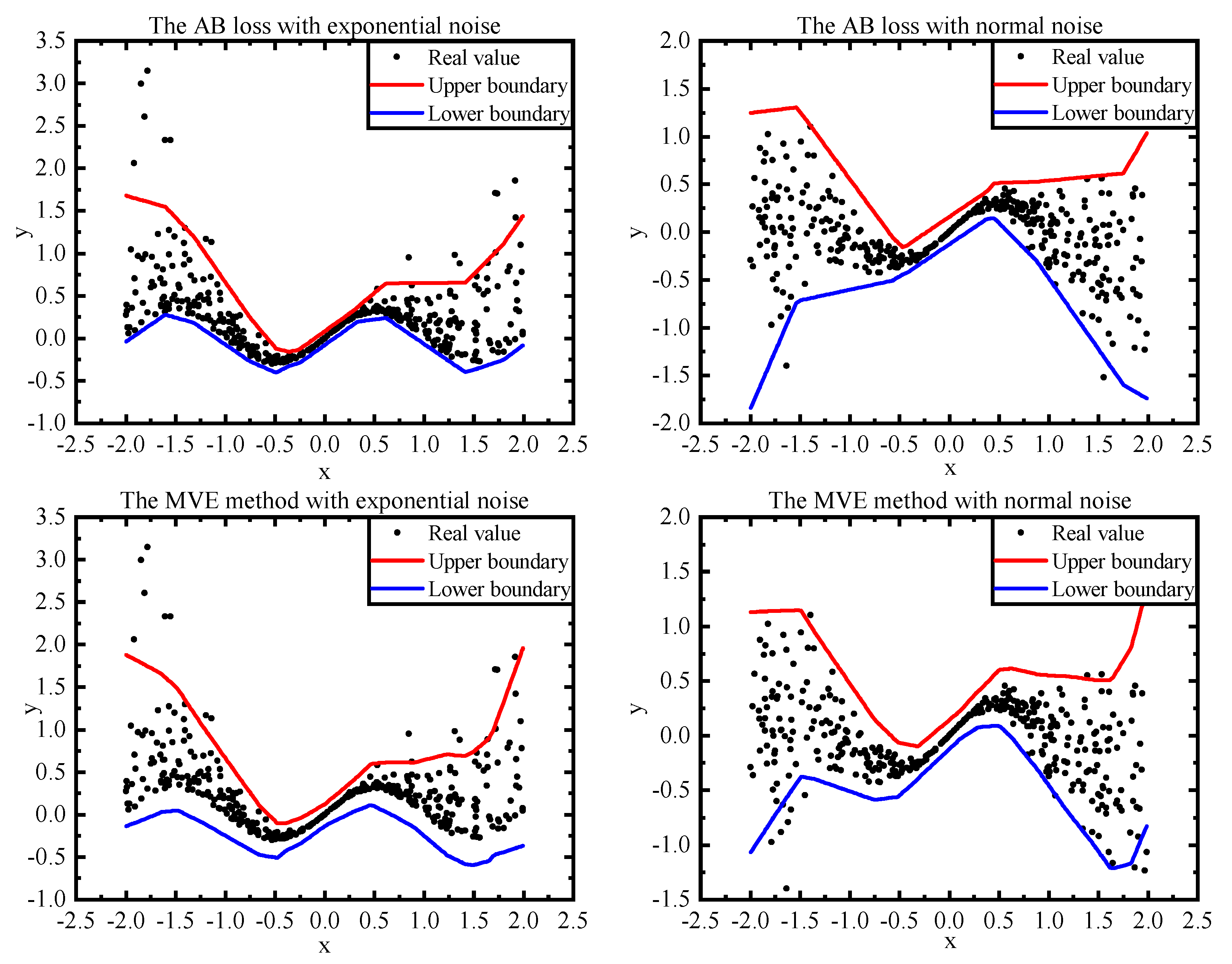
Figure 4 shows the results of the MVE method and the AB loss under various types of noise. According to the results, the MVE outputs PIs close to the generated data for normal noise, but struggles with exponential noise, while the AB loss approximates both reasonably. Such results are consistent with the assumption of the variance distribution in the MVE method. They also verified that the AB loss may not be restricted by the variance distribution, which is more flexible than the MVE method.

According to

Table 4. Statistical characteristics of PICP, MPIW and CWC for the LUBE method, the QD loss and the AB loss in 8 benchmark experiments.

Case Study	LUBE Method		QD Loss			AB Loss
	PICP (%)	MPIW	PICP (%)	MPIW	CWC	PICP (%)	MPIW	CWC
#3	94.07	5.89	95.00	1.15	344.00	96.00	1.16	355.90
#4	94.17	4.98	95.60	1.34	141.20	95.60	1.41	150.00
#5	96.09	4.19	96.10	1.16	86.57	100.00	0.73	72.71
#6	94.90	5.33	95.10	1.72	786.90	96.80	1.68	760.66
#7	92.37	3.42	96.70	3.23	300.90	100.00	3.38	314.70
#8	95.13	3.72	95.80	0.99	339.40	95.40	0.94	321.30
#9	94.00	6.90	95.70	4.42	562.60	97.80	3.85	500.30
#10	96.10	5.31	100.00	0.37	26.10	98.39	0.28	18.96

, the MPIW of the QD loss and the AB loss with GD is smaller than the LUBE method with PSO, which indicates that the QD loss and the AB loss can generate higher quality PIs. Due to the heuristic search algorithm, it is difficult to find the optimal result in a limited time when there is no restriction on the data. Therefore, the implemented LUBE method performed poorly in the experiment. According to the CWC metric values, in case study 3, 4 and 7, the performance of the QD loss is slightly better than the AB loss while in other cases, the AB loss gives a better performance. The result confirms that the AB loss can generate high-quality PIs in regression tasks.

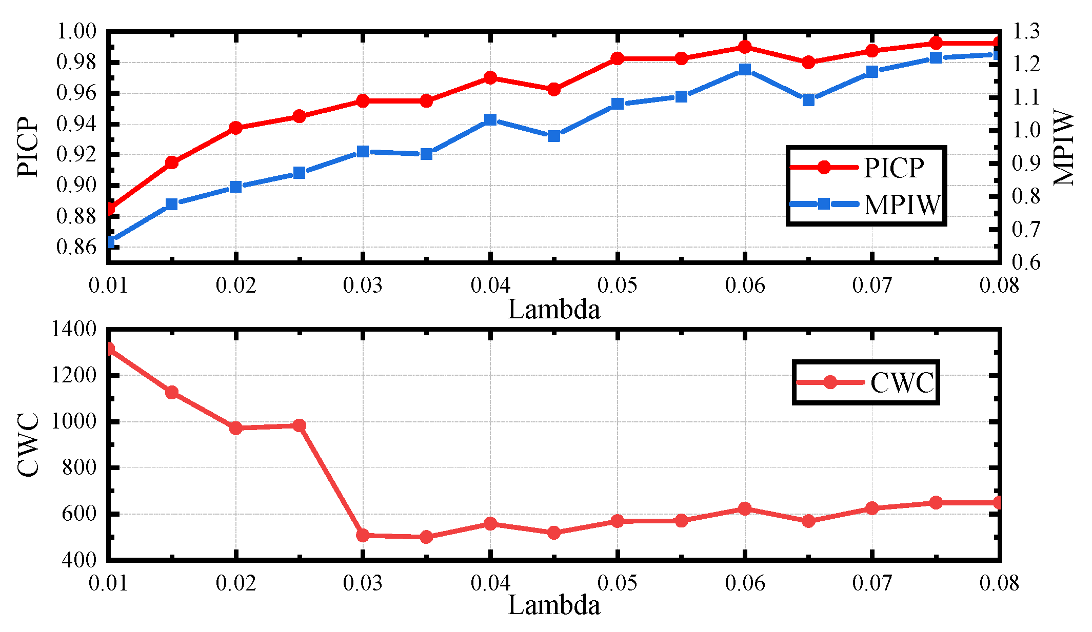
The weight parameter is vital for model training, which determines the quality of PI generated by the trained model. By adjusting the weight parameters, the importance between confidence and sharpness can be determined. A good model should be sensitive to the change of the weight parameter, which makes it more convenient for parameter adjusting.

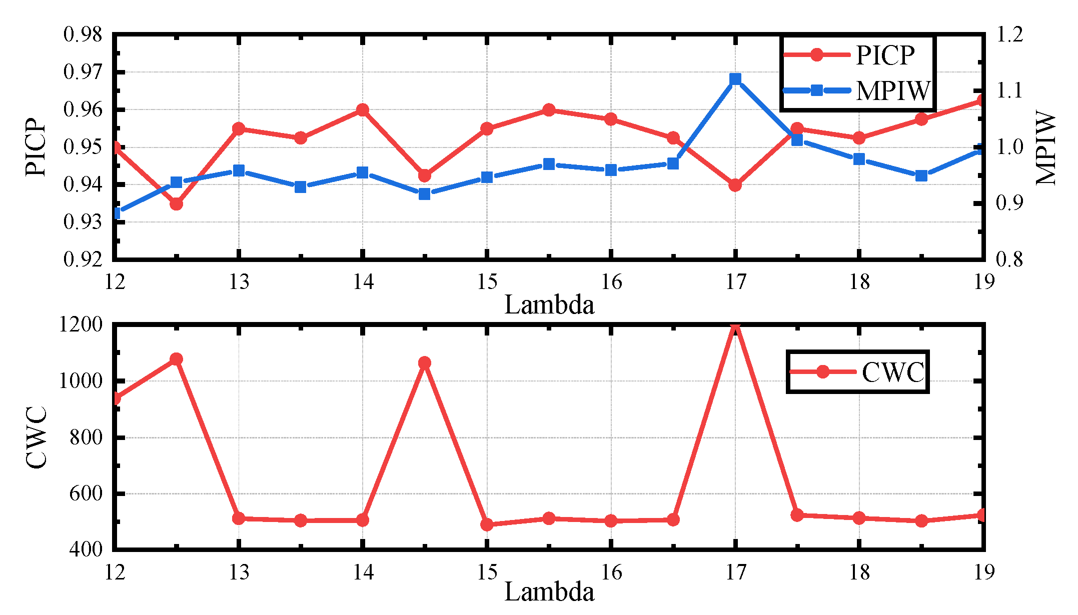
Figure 5 and Figure 6 illustrate the relationship between the weight parameter and the metric values obtained after convergence when using the AB loss and the QD loss. With the increase of the weight parameter, the PICP obtained by the AB loss increases and approaches 1, while the PICP obtained by the QD loss oscillates.

4. Discussions

Case study 1 demonstrates that the model trained by the AB loss obtains higher quality PIs under samples of all batch sizes if compared with the QD loss. According to Table 3, the model obtained by QD loss does not fit the superimposed noise well for batch sizes of 16 and 32. The performance of the QD loss improves gradually with the increasing of batch size for training. This implies that the QD loss may be inadaptable to small sample sets, while the AB loss performs well for all batch sizes. The AB loss takes advantage of the direct application of the Taylor expansion to approximation, without the necessity of changing the basic assumption of the binomial distribution, which allows it to solve more practical problems while ensuring accuracy.

Many traditional PI construction methods were built based on the various assumptions regarding data distribution, which may be unsatisfied in real-world datasets. However, as a distribution-free method, the AB loss is more suitable for practical applications. As shown in Figure 4, compared with traditional methods such as MVE, more reasonable results may be obtained when different noises are added to the dataset. Thus, there is no limitation on data distribution when utilizing the AB loss for model training. The results of numerical experiments also prove that the AB loss can obtain higher quality PIs than existing state-of-the-art methods in most cases.

In addition, it can be seen that the AB loss is more sensitive to confidence measurement than the QD loss, which indicates that the PIs generated by the proposed method are more likely to meet the required confidence level. When utilizing the AB loss, more energy should be devoted to sharpness measurement, which may result in high quality PIs. Meanwhile, from the curves of CWC with weight parameters in Figure 5 and Figure 6, it can be seen that the best parameters are easier to find when adopting AB loss, which simplifies the parameter adjustment process and makes it more convenient to deploy in practice.

In summary, the results prove the reliability and the quality of PIs constructed by the AB loss. By introducing the AB loss into the PI generation model, it is possible to use small batches for model training, which is appropriate in many real-world tasks.

Future works may be investigated in the following aspects:

• The realization of the AB loss in this study did not consider the impact of model uncertainty. Since two networks are used to predict the prediction estimate and the bias estimate, the uncertainty of the model was not determined in the implementation. It is possible to use methods such as bootstrap to estimate model uncertainty to improve the quality of the results;
• The existence of the penalty term means it is not necessary to initialize the model before the training process, although this feature increases the computational complexity. More efforts should be made to simplify the penalty term;
• It is difficult to adjust the weight parameter of the AB loss on different datasets. A more efficient way should be explored to balance the contradiction between confidence and sharpness.

5. Conclusions

An all-batch (AB) loss function is proposed in this work for the construction of PIs, and a high-reliability PI generation framework is constructed to generate PIs as well as point estimates based on the proposed AB loss and the dual-FNN structure. The proposed AB loss avoids restriction on the data scale in QD loss, which makes it suitable for small batches. By taking full advantage of likelihood theory, the proposed scheme can perform well under all batch sizes of samples. A comparison among the MVE method, the LUBE method, the QD loss and the AB loss was conducted to prove the flexibility and effectiveness of the proposed scheme. The proposed scheme was advantageous in terms of its strong adaptability, simple structure and high degree of stability, and may thus be applicable to solve various practical problems, such as wind speed forecasts, landslide displacement, electricity load predictions, etc. By combining various advanced machine learning technologies such as cross validation, pruning, dropout, etc., the quality of constructed prediction intervals may be further enhanced.

References

- Meade, N.; Islam, T. Prediction intervals for growth curve forecasts. J. Forecast. 1995, 14, 413–430. [Google Scholar] [CrossRef]
- Shen, Y.; Wang, X.; Chen, J. Wind power forecasting using multi-objective evolutionary algorithms for wavelet neural network optimized prediction intervals. Appl. Sci. 2018, 8, 185. [Google Scholar] [CrossRef] [Green Version]
- Wan, C.; Zhao, C.; Song, Y. Chance constrained extreme learning machine for nonparametric prediction intervals of wind power generation. IEEE Trans. Power Syst. 2020, 35, 3869–3884. [Google Scholar] [CrossRef]
- Wu, Y.-K.; Wu, Y.-C.; Hong, J.-S.; Phan, L.-H.; Phan, Q.-D. Probabilistic forecast of wind power generation with data processing and numerical weather predictions. IEEE Trans. Ind. Appl. 2020, 57, 36–45. [Google Scholar] [CrossRef]
- Mykhailovych, T.; Fryz, M. Model and information technology for hourly water consumption interval forecasting. In Proceedings of the IEEE 15th International Conference on Advanced Trends in Radioelectronics, Telecommunications and Computer Engineering, Lviv-Slavske, Ukraine, 25–29 February 2020; pp. 341–345. [Google Scholar]
- Du, S.; Wu, M.; Chen, L.; Hu, J.; Cao, W.; Pedrycz, W. Operating mode recognition based on fluctuation interval prediction for iron ore sintering process. IEEE/ASME Trans. Mechatron. 2020, 25, 2297–2308. [Google Scholar] [CrossRef]
- Zheng, L.; Xiao, X.; Sun, B.; Mei, D.; Peng, B. Short-term parking demand prediction method based on variable prediction interval. IEEE Access. 2020, 8, 58594–58602. [Google Scholar] [CrossRef]
- Cheng, J.; Duan, D.; Cheng, X.; Yang, L.; Cui, S. Adaptive control for energy exchange with probabilistic interval predictors in isolated microgrids. Energies 2021, 14, 375. [Google Scholar] [CrossRef]
- Kurt, H.; Maxwell, S.; Halbert, W. Multilayer feedforward networks are universal approximators. Neural Netw. 1989, 2, 359–366. [Google Scholar]
- Chryssolouris, G.; Lee, M.; Ramsey, A. Confidence interval prediction for neural network models. IEEE Trans. Neural Netw. 1996, 7, 229–232. [Google Scholar] [CrossRef]
- Hwang, J.T.G.; Ding, A.A. Prediction intervals for artificial neural networks. J. Am. Stat. Assoc. 1997, 92, 748–757. [Google Scholar] [CrossRef]
- Bishop, C.M. Neural Networks for Pattern Recognition; Oxford University Press: London, UK, 1995. [Google Scholar]
- MacKay, D.D.J.C. The evidence framework applied to classification networks. Neural Comput. 1992, 4, 720–736. [Google Scholar] [CrossRef]
- Heskes, T. Practical confidence and prediction intervals. In Proceedings of the 1997 Conference on Advance in Neural Information Processing Systems; MIT Press: Cambridge, MA, USA, 1997; pp. 176–182. [Google Scholar]
- Carney, J.G.; Cunningham, P.; Bhagwan, U. Confidence and prediction intervals for neural network ensembles. In Proceedings of the International Joint Conference on Neural Networks, Washington, DC, USA, 10–16 July 1999; pp. 1215–1218. [Google Scholar]
- Errouissi, R.; Cárdenas-Barrera, J.L.; Meng, J.; Guerra, E.C. Bootstrap prediction interval estimation for wind speed forecasting. In Proceedings of the IEEE Energy Conversion Congress and Exposition, Montreal, QC, Canada, 20–24 September 2015; pp. 1919–1924. [Google Scholar]
- Mancini, T.; Pardo, H.C.; Olmo, J. Prediction intervals for deep neural networks. arXiv 2020, arXiv:2010.04044. [Google Scholar]
- Dybowski, R.; Roberts, S.J. Confidence Intervals and Prediction Intervals for Feed-Forward Neural Networks; Cambridge University Press: Cambridge, UK, 2001. [Google Scholar]
- Nix, D.A.; Weigend, A.S. Estimating the mean and variance of the target probability distribution. In Proceedings of the IEEE International Conference on Neural Networks, Orlando, FL, USA, 28 June–2 July 1994; pp. 55–60. [Google Scholar]
- Khosravi, A.; Nahavandi, S.; Creighton, D.; Atiya, A.F. Lower upper bound estimation method for construction of neural network-based prediction intervals. IEEE Trans. Neural Netw. 2010, 22, 337–346. [Google Scholar] [CrossRef] [PubMed]
- Ak, R.; Li, Y.-F.; Vitelli, V.; Zio, E. Multi-Objective Genetic Algorithm Optimization of a Neural Network for Estimating Wind Speed Prediction Intervals; hal-00864850; HAL: Paris, France, 2013; Unpublished work. [Google Scholar]
- Wang, J.; Fang, K.; Pang, W.; Sun, J. Wind power interval prediction based on improved PSO and BP neural network. J. Electr. Eng. Technol. 2017, 12, 989–995. [Google Scholar] [CrossRef] [Green Version]
- Long, H.; Zhang, C.; Geng, R.; Wu, Z.; Gu, W. A combination interval prediction model based on biased convex cost function and auto rncoder in solar power prediction. IEEE Trans. Sustain. Energy 2021. [Google Scholar] [CrossRef]
- Goodfellow, I.; Bengio, Y.; Courville, A. Deep Learning; MIT Press: Cambridge, MA, USA, 2016. [Google Scholar]
- Pearce, T.; Zaki, M.; Brintrup, A.M.; Neely, A. High-quality prediction intervals for deep learning: A distribution-free, ensembled approach. In Proceedings of the 35th International Conference on Machine Learning, Stockholm, Sweden, 10–15 July 2018; pp. 4075–4084. [Google Scholar]
- Hoffer, E.; Hubara, I.; Soudry, D. Train longer, generalize better: Closing the generalization gap in large batch training of neural networks. In Proceedings of the Advances in Neural Information Processing Systems, Long Beach, CA, USA, 4–9 December 2017; pp. 1731–1741. [Google Scholar]
- Liu, D.; He, Z.; Chen, D.; Lv, J. A network framework for small-sample learning. IEEE Trans. Neural Netw. Learn. Syst. 2020, 31, 4049–4062. [Google Scholar] [CrossRef]
- Salem, T.S.; Langseth, H.; Ramampiaro, H. Prediction intervals: Split normal mixture from quality-driven deep ensemble. arXiv 2020, arXiv:2007.09670v1. [Google Scholar]
- Khosravi, A.; Nahavandi, S.; Creighton, D.; Atiya, A.F. Comprehensive review of neural network-based prediction intervals and new advances. IEEE Trans. Neural Netw. 2011, 22, 1341–1356. [Google Scholar] [CrossRef] [PubMed]
- Khosravi, A.; Nahavandi, S.; Creighton, D. A prediction interval based approach to determine optimal structures of neural network metamodels. Expert Syst. Appl. 2010, 37, 2377–2387. [Google Scholar] [CrossRef]
- Shrestha, D.L.; Solomatine, D.P. Machine learning approaches for estimation of prediction interval for the model output. Neural Netw. 2006, 19, 225–235. [Google Scholar] [CrossRef]
- Laarhoven, P.J.M.V.; Aarts, E.H.L. Simulated Annealing: Theory and Applications; Kluwer: Boston, UK, 1987. [Google Scholar]
- Harrison, D.; Rubinfeld, D. Hedonic housing prices and the demand for clean air. J. Environ. Econ. Manag. 1978, 5, 81–102. [Google Scholar] [CrossRef] [Green Version]
- Yeh, I.-C. Modeling of strength of high-performance concrete using artificial neural networks. Cem. Concr. Res. 1998, 28, 1797–1808. [Google Scholar] [CrossRef]
- Tsanas, A.; Xifara, A. Accurate quantitative estimation of energy performance of residential buildings using statistical machine learning tools. Energy Build. 2012, 49, 560–567. [Google Scholar] [CrossRef]
- Corke, P.I. A robotics toolbox for MATLAB. IEEE Robot. Autom. Mag. 1996, 3, 24–32. [Google Scholar] [CrossRef] [Green Version]
- Coraddu, A.; Oneto, L.; Ghio, A.; Savio, S.; Anguita, D.; Figari, M. Machine learning approaches for improving condition-based maintenance of naval propulsion plants. J. Eng. Maritime Environ. 2014, 230, 136–153. [Google Scholar] [CrossRef]
- Altosole, M.; Benvenuto, G.; Figari, M.; Campora, U. Real-time simulation of a cogag naval ship propulsion system. J. Eng. Maritime Environ. 2009, 223, 47–62. [Google Scholar] [CrossRef]
- Tüfekci, P. Prediction of full load electrical power output of a base load operated combined cycle power plant using machine learning methods. Int. J. Electr. Power Energy Syst. 2014, 60, 126–140. [Google Scholar] [CrossRef]
- Kaya, H.; Tüfekci, P.; Gürgen, S.F. Local and hlobal learning methods for predicting power of a xombined gas & steam turbine. In Proceedings of the International Conference on Emerging Trends in Computer and Electronics Engineering, Dubai, United Arab Emirates, 24–25 March 2012; pp. 13–18. [Google Scholar]
- Cortez, P.; Cerdeira, A.; Almeida, F.; Matos, T. Modeling wine preferences by data mining from physicochemical properties. Decis. Support Syst. 2009, 47, 547–553. [Google Scholar] [CrossRef] [Green Version]
- Gerritsma, J.; Onnink, R.; Versluis, A. Geometry, resistance and stability of the Delft systematic yacht hull series1. Int. Shipbuild. Prog. 1981, 28, 276–286. [Google Scholar] [CrossRef]
- Kingma, D.P.; Ba, J. Adam: A method for stochastic optimization. arXiv 2014, arXiv:1412.6980. [Google Scholar]
- Ye, L.; Zhou, J.; Gupta, H.V.; Zhang, H. Efficient estimation of flood forecast prediction intervals via single and multi-objective versions of the LUBE method. Hydrol. Process. 2016, 30, 2703–2716. [Google Scholar] [CrossRef]
Figure 1.
Schematic of the proposed framework for construction of PIs.
Figure 2.
Comparison of PI boundaries for the AB loss by changing the batch size. The upper and lower boundaries are the predicted 95% PIs. The predicted value is generated by the prediction network in the framework.
Figure 3.
Comparison of PI boundaries for the QD loss by changing the batch size. The upper and lower boundaries are the predicted 95% PIs. The predicted value is generated by the prediction network in the framework.
Figure 4.
Comparison of PI boundaries for the MVE method and the AB loss under normal noise and exponential noise. The upper and lower boundaries are the predicted 95% PIs.
Figure 5.
Relationship between the weight parameter and the value of PICP, MPIW and CWC when using AB loss.
Figure 6.
Relationship between the weight parameter and the value of PICP, MPIW and CWC when using QD loss.