
Low-Power Beam-Switching Technique for Power-Efficient Collaborative IoT Edge Devices


Abstract
:1. Introduction
2. System Model and Motivation
3. Proposed Algorithm
- Step 1:
- Initialization. As the first step of the algorithm, one of the active sensors, s, sets the control parameters of the algorithm, , , and as the default values. These values are important to balance between SNR improvement and system complexity.
- Step 2:
- Broadcasting.s broadcasts a switching message to alert the following beam-switching event to the neighbor sensors.
- Step 3:
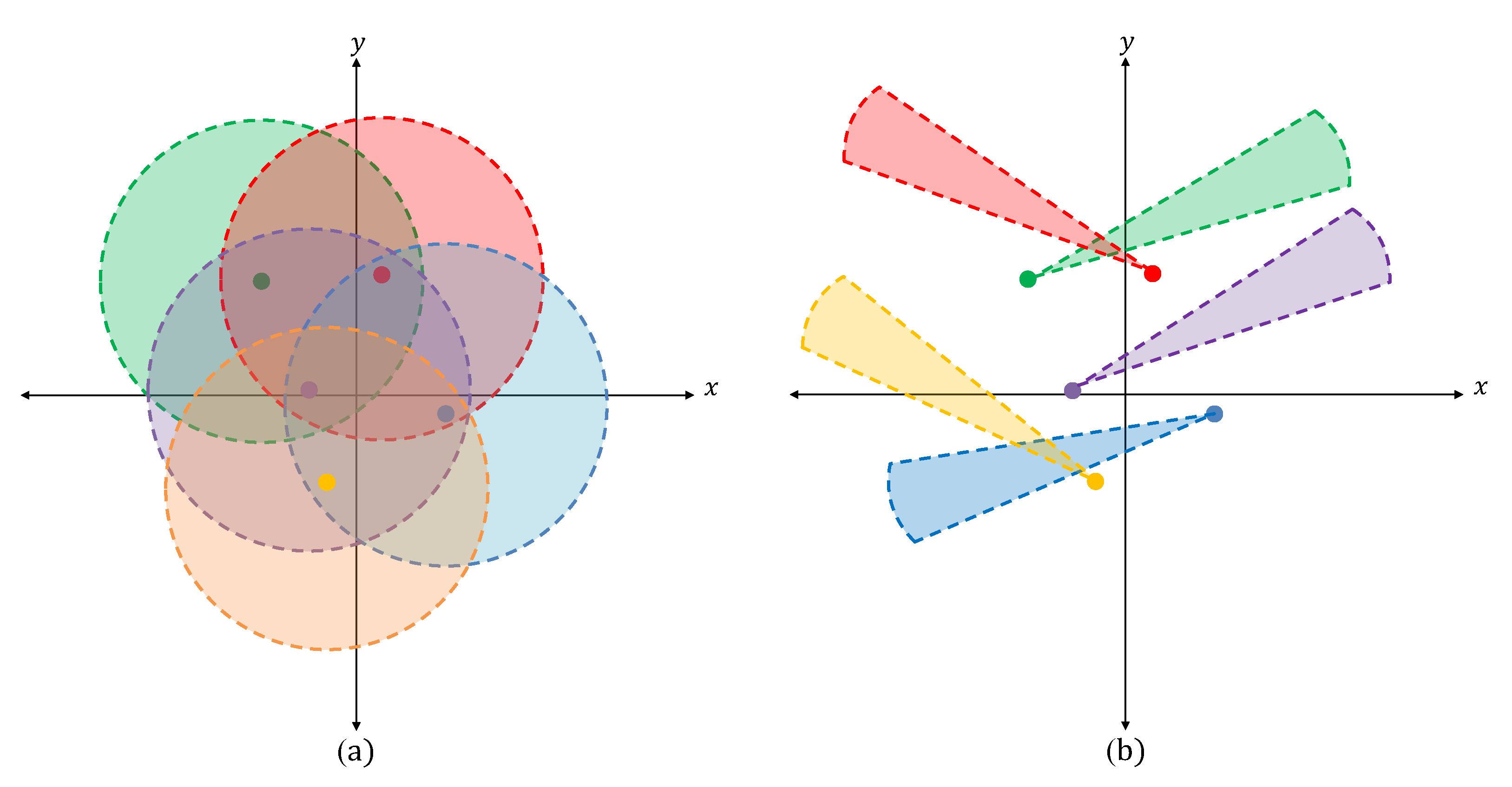
- Beam Switching. After receiving the switching message, each sensor randomly selects one of the directional beams, being generated from its own BSS, with and sends a selected message to s.
- Step 4:
- Data Sharing. After collecting the selected messages from the neighbor sensors, s shares its transmission data with them. When each of the sensors receives the data, it sends a shared message to s.
- Step 5:
- Sounding. (1) After collecting the shared messages from the neighboring sensors, s with transmits a sounding message with the shared data through the CB. Here, it is assumed that s and are synchronized. measures and feeds it back to s. (2) If is larger than the predetermined threshold SNR, , or is met, then go to Step 7 directly.
- Step 6:
- Updating. If is available, s makes the decision for either the acceptance or rejection of the state transition. If it is not available, then go back to (1) of Step 5. When the transition is accepted, is replaced with . Then, return to Step 2, and s repeats from Step 2 to Step 6 during iterations.
- Step 7:
- Abort. Check whether all iterations have stopped or is met. If either of these conditions are true, s broadcasts an abort message, and uses the set of beams having for the future data transmission.
4. Simulations and Experiments
5. Conclusions
Author Contributions
Funding
Conflicts of Interest
Abbreviations
| WSN | Wireless Sensor Network |
| AP | Access Point |
| CB | Collaborative Beamforming |
| BSS | Beam-Switching Structures |
| SNR | Signal-to-Noise Ratio |
| GS | Greedy Search |
| RF-MEMS | Radio-Frequency Micro-Electromechanical Systems |
| GPS | Global Positioning System |
| MCU | Micro Controller Unit |
| UART | Universal Asynchronous Receiver Transmitter |
References
- Ayaz, M.; Ammad-Uddin, M.; Baig, I. Wireless sensor’s civil applications, prototypes, and future integration possibilities: A review. IEEE Sens. J. 2017, 18, 4–30. [Google Scholar] [CrossRef]
- Noel, A.B.; Abdaoui, A.; Elfouly, T.; Ahmed, M.H.; Badawy, A.; Shehata, M.S. Structural health monitoring using wireless sensor networks: A comprehensive survey. Commun. Surv. Tutor. 2017, 19, 1403–1423. [Google Scholar] [CrossRef]
- Salari, S.; Kim, I.M.; Chan, F. Distributed cooperative localization for mobile wireless sensor networks. IEEE Wirel. Commun. Lett. 2017, 7, 18–21. [Google Scholar] [CrossRef]
- Thomas, D.; Shankaran, R.; Orgun, M.; Hitchens, M.; Ni, W. Energy-efficient military surveillance: Coverage meets connectivity. IEEE Sens. J. 2019, 19, 3902–3911. [Google Scholar] [CrossRef]
- Olasupo, T.O. Wireless Communication Modeling for the Deployment of Tiny IoT Devices in Rocky and Mountainous Environments. IEEE Sens. Lett. 2019, 3, 1–4. [Google Scholar] [CrossRef]
- Liu, J.; Liu, H.; Chen, Y.; Wang, Y.; Wang, C. Wireless sensing for human activity: A survey. IEEE Commun. Surv. Tutor. 2019, 22, 1629–1645. [Google Scholar] [CrossRef]
- Saeed, N.; Alouini, M.S.; Al-Naffouri, T.Y. Toward the internet of underground things: A systematic survey. IEEE Commun. Surv. Tutor. 2019, 21, 3443–3466. [Google Scholar] [CrossRef] [Green Version]
- Jouhari, M.; Ibrahimi, K.; Tembine, H.; Ben-Othman, J. Underwater wireless sensor networks: A survey on enabling technologies, localization protocols, and internet of underwater things. IEEE Access 2019, 7, 96879–96899. [Google Scholar] [CrossRef]
- Wong, D.; Yu, J.; Li, Y.; Deepu, C.; Ngo, D.; Zhou, C.; Shashi, R.; Koh, A.; Hong, R.; Veeravalli, B.; et al. An Integrated Wearable Wireless Vital Signs Biosensor for Continuous Inpatient Monitoring. IEEE Sens. J. 2019, 20, 448–462. [Google Scholar] [CrossRef]
- Khutsoane, O.; Isong, B.; Gasela, N.; Abu-Mahfouz, A.M. WaterGrid-Sense: A LoRa-based Sensor Node for Industrial IoT applications. IEEE Sens. J. 2019, 20, 2722–2729. [Google Scholar] [CrossRef]
- Zhang, Z.; Glaser, S.; Watteyne, T.; Malek, S. Long-term monitoring of the Sierra Nevada snowpack using wireless sensor networks. IEEE Internet Things J. 2020. [Google Scholar] [CrossRef] [Green Version]
- Li, J.; Xing, Z.; Zhang, W.; Lin, Y.; Shu, F. Vehicle Tracking in Wireless Sensor Networks via Deep Reinforcement Learning. IEEE Sens. Lett. 2020, 4, 1–4. [Google Scholar] [CrossRef]
- Xu, G.; Wang, F.; Zhang, M.; Peng, J. Efficient and Provably Secure Anonymous User Authentication Scheme for Patient Monitoring Using Wireless Medical Sensor Networks. IEEE Access 2020, 8, 47282–47294. [Google Scholar] [CrossRef]
- Yu, B.; Choi, W.; Lee, T.; Kim, H. Clustering Algorithm Considering Sensor Node Distribution in Wireless Sensor Networks. J. Inf. Process. Syst. 2018, 14, 926–940. [Google Scholar]
- Rao, S.; Shama, K.; Kumar, P. Energy efficient Cross Layer Multipath Routing for Image Delivery in Wireless Sensor Networks. J. Inf. Process. Syst. 2018, 14, 1347–1360. [Google Scholar]
- Wan, R.; Xiong, N.; Nguyen the Loc. An energy-efficient sleep scheduling mechanism with similarity measure for wireless sensor networks. Hum. Centric Comput. Inf. Sci. 2018, 8, 18. [Google Scholar] [CrossRef] [Green Version]
- Rhim, H.; Tamine, K.; Abassi, R.; Sauveron, D.; Guemara, S. A multi-hop graph-based approach for an energy-efficient routing protocol in wireless sensor networks. Hum. Centric Comput. Inf. Sci. 2018, 8, 1–21. [Google Scholar] [CrossRef]
- Lee, D.; Moon, H.; Oh, S.; Park, D. mIoT: Metamorphic IoT Platform for On-Demand Hardware Replacement in Large-Scaled IoT Applications. Sensors 2020, 20, 3337. [Google Scholar] [CrossRef] [PubMed]
- Zhang, Z.; Mao, X.; Zhou, K.; Yuan, H. Collaborative sensing based parking tracking system with wireless magnetic sensor network. IEEE Sens. J. 2020, 20, 4859–4867. [Google Scholar] [CrossRef]
- Lee, M.; Kwan, T.; Hara, S.; Morimoto, K.; Suzuki, Y. Development of Flexible Wireless Wall Temperature Sensor for Combustion Studies. IEEE Sens. Lett. 2019, 3, 1–4. [Google Scholar] [CrossRef]
- Moallem, M.M.; Aghagolzadeh, A.; Ghazalian, R. Wireless Visual Sensor Networks Energy Optimization Based on New Entropy Model. IEEE Sens. J. 2019, 20, 778–785. [Google Scholar] [CrossRef]
- Gochoo, M.; Tan, T.H.; Huang, S.C.; Batjargal, T.; Hsieh, J.W.; Alnajjar, F.S.; Chen, Y.F. Novel IoT-Based Privacy-Preserving Yoga Posture Recognition System Using Low-Resolution Infrared Sensors and Deep Learning. IEEE Internet Things J. 2019, 6, 7192–7200. [Google Scholar] [CrossRef]
- Zhang, J.; Wu, P. Joint Sampling Synchronization and Source Localization for Wireless Acoustic Sensor Networks. IEEE Commun. Lett. 2020, 24, 1020–1023. [Google Scholar] [CrossRef]
- Wang, R.; Ma, J.J.; Chen, C.S.; Wang, B.Z.; Xiong, J. Low-profile Implementation of U-Shaped Power Quasi-Isotropic Antennas for Intra-Vehicle Wireless Communications. IEEE Access 2020, 8, 48557–48565. [Google Scholar] [CrossRef]
- Wang, Q.; Dai, H.N.; Zheng, Z.; Imran, M.; Vasilakos, A.V. On connectivity of wireless sensor networks with directional antennas. Sensors 2017, 17, 134. [Google Scholar] [CrossRef] [Green Version]
- Skiani, E.; Mitilineos, S.; Thomopoulos, S. A study of the performance of wireless sensor networks operating with smart antennas. IEEE Antennas Propag. Mag. 2012, 54, 50–67. [Google Scholar] [CrossRef]
- Zhang, J.; Jia, X.; Zhou, Y. Analysis of capacity improvement by directional antennas in wireless sensor networks. ACM Trans. Sens. Netw. 2012, 9, 1–26. [Google Scholar] [CrossRef]
- Dai, H.N.; Ng, K.W.; Li, M.; Wu, M.Y. An overview of using directional antennas in wireless networks. Int. J. Commun. Syst. 2013, 26, 413–448. [Google Scholar] [CrossRef]
- Duan, Z.; Tao, L.; Zhang, X. Energy Efficient Data Collection and Directional Wireless Power Transfer in Rechargeable Sensor Networks. IEEE Access 2019, 7, 178466–178475. [Google Scholar] [CrossRef]
- Constantine, A.B. Antenna Theory: Analysis and Design, 3rd ed.; John Wiley & Sons: New York, NY, USA, 2016. [Google Scholar]
- Dong, L.; Petropulu, A.P.; Poor, H.V. A cross-layer approach to collaborative beamforming for wireless ad hoc networks. IEEE Trans. Signal Process. 2008, 56, 2981–2993. [Google Scholar] [CrossRef]
- Cheng, S.; Rantakari, P.; Malmqvist, R.; Samuelsson, C.; Vaha-Heikkila, T.; Rydberg, A.; Varis, J. Switched beam antenna based on RF MEMS SPDT switch on quartz substrate. IEEE Antennas Wirel. Propag. Lett. 2009, 8, 383–386. [Google Scholar] [CrossRef]
- Vasylchenko, A.; Fernández-Bolaños, M.; Brebels, S.; De Raedt, W.; Vandenbosch, G.A. Conformal phased array for a miniature wireless sensor node. In Proceedings of the 2010 Conference Proceedings ICECom, Dubrovnik, Croatia, 20–23 September 2010; pp. 1–4. [Google Scholar]
- Luo, Y.; Kikuta, K.; Han, Z.; Takahashi, T.; Hirose, A.; Toshiyoshi, H. An active metamaterial antenna with MEMS-modulated scanning radiation beams. IEEE Electron Device Lett. 2016, 37, 920–923. [Google Scholar] [CrossRef]
- Catarinucci, L.; Guglielmi, S.; Colella, R.; Tarricone, L. Compact switched-beam antennas enabling novel power-efficient wireless sensor networks. IEEE Sens. J. 2014, 14, 3252–3259. [Google Scholar] [CrossRef]
- Shen, X.; Liu, Y.; Zhao, L.; Huang, G.L.; Shi, X.; Huang, Q. A Miniaturized Microstrip Antenna Array at 5G Millimeter-Wave Band. IEEE Antennas Wirel. Propag. Lett. 2019, 18, 1671–1675. [Google Scholar] [CrossRef]
- Catarinucci, L.; Guglielmi, S.; Patrono, L.; Tarricone, L. Switched-beam antenna for wireless sensor network nodes. Prog. Electromagn. Res. 2013, 39, 193–207. [Google Scholar] [CrossRef] [Green Version]
- Boukerche, A.; Wu, Q.; Sun, P. Efficient Green Protocols for Sustainable Wireless Sensor Networks. IEEE Trans. Sustain. Comput. 2019, 5, 61–80. [Google Scholar] [CrossRef]
- Wu, Y.; He, Y.; Shi, L. Energy-saving Measurement in LoRaWAN Based Wireless Sensor Networks by Using Compressed Sensing. IEEE Access 2020, 8, 49477–49486. [Google Scholar] [CrossRef]
- Sambo, D.W.; Förster, A.; Yenke, B.O.; Sarr, I.; Gueye, B.; Dayang, P. Wireless Underground Sensor Networks Path Loss Model for Precision Agriculture (WUSN-PLM). IEEE Sens. J. 2020, 20, 5298–5313. [Google Scholar] [CrossRef]
- Ochiai, H.; Mitran, P.; Poor, H.V.; Tarokh, V. Collaborative beamforming for distributed wireless ad hoc sensor networks. IEEE Trans. Signal Process. 2005, 53, 4110–4124. [Google Scholar] [CrossRef] [Green Version]
- Ahmed, M.F.; Vorobyov, S.A. Collaborative beamforming for wireless sensor networks with Gaussian distributed sensor nodes. IEEE Trans. Wireless Commun. 2009, 8, 638–643. [Google Scholar] [CrossRef]
- Huang, J.; Wang, P.; Wan, Q. Collaborative beamforming for wireless sensor networks with arbitrary distributed sensors. IEEE Commun. Lett. 2012, 16, 1118–1120. [Google Scholar] [CrossRef]
- Park, D.; Youn, J.; Cho, J. A Low-Power Microcontroller with Accuracy-Controlled Event-Driven Signal Processing Unit for Rare-Event Activity-Sensing IoT Devices. J. Sens. 2015, 2015, 1–10. [Google Scholar] [CrossRef] [Green Version]
- Haro, B.B.; Zazo, S.; Palomar, D.P. Energy efficient collaborative beamforming in wireless sensor networks. IEEE Trans. Signal Process. 2013, 62, 496–510. [Google Scholar] [CrossRef]
- Chen, J.C.; Wen, C.K.; Wong, K.K. An efficient sensor-node selection algorithm for sidelobe control in collaborative beamforming. IEEE Trans. Veh. Technol. 2015, 65, 5984–5994. [Google Scholar] [CrossRef]
- Jayaprakasam, S.; Rahim, S.K.A.; Leow, C.Y.; Ting, T.O.; Eteng, A.A. Multiobjective beampattern optimization in collaborative beamforming via NSGA-II with selective distance. IEEE Trans. Antennas Propag. 2017, 65, 2348–2357. [Google Scholar] [CrossRef]
- Kurt, S.; Tavli, B. Path-Loss Modeling for Wireless Sensor Networks: A review of models and comparative evaluations. IEEE Antennas Propag. Mag. 2017, 59, 18–37. [Google Scholar] [CrossRef]
- Jayaprakasam, S.; Rahim, S.K.A.; Leow, C.Y. Distributed and collaborative beamforming in wireless sensor networks: Classifications, trends, and research directions. IEEE Commun. Surv. Tutor. 2017, 19, 2092–2116. [Google Scholar] [CrossRef]
- Sun, G.; Liu, Y.; Liang, S.; Chen, Z.; Wang, A.; Ju, Q.; Zhang, Y. A sidelobe and energy optimization array node selection algorithm for collaborative beamforming in wireless sensor networks. IEEE Access 2017, 6, 2515–2530. [Google Scholar] [CrossRef]
- Duraisamy, S.; Pugalendhi, G.K.; Balaji, P. Reducing energy consumption of wireless sensor networks using rules and extreme learning machine algorithm. J. Eng. 2019, 2019, 5443–5448. [Google Scholar] [CrossRef]
- Liang, S.; Fang, Z.; Sun, G.; Liu, Y.; Zhao, X.; Qu, G.; Zhang, Y.; Leung, V.C. JSSA: Joint Sidelobe Suppression Approach for Collaborative Beamforming in Wireless Sensor Networks. IEEE Access 2019, 7, 151803–151817. [Google Scholar] [CrossRef]
- Bao, X.; Liang, H.; Liu, Y.; Zhang, F. A Stochastic Game Approach for Collaborative Beamforming in SDN-Based Energy Harvesting Wireless Sensor Networks. IEEE Internet Things J. 2019, 6, 9583–9595. [Google Scholar] [CrossRef]
- Jung, H.; Lee, I.H. Secrecy performance analysis of analog cooperative beamforming in three-dimensional Gaussian distributed wireless sensor networks. IEEE Trans. Wirel. Commun. 2019, 18, 1860–1873. [Google Scholar] [CrossRef]
- Sun, G.; Liu, Y.; Chen, Z.; Wang, A.; Zhang, Y.; Tian, D.; Leung, V.C. Energy Efficient Collaborative Beamforming for Reducing Sidelobe in Wireless Sensor Networks. IEEE Trans. Mob. Comput. 2019, 20, 965–982. [Google Scholar] [CrossRef]
- Berbakov, L.; Dimić, G.; Beko, M.; Vasiljević, J.; Stojković, Ž. Collaborative Data Transmission in Wireless Sensor Networks. IEEE Access 2020, 8, 39647–39658. [Google Scholar] [CrossRef]
- Kim, S.; Cho, J.; Park, D. Moving-Target Position Estimation Using GPU-Based Particle Filter for IoT Sensing Applications. Appl. Sci. 2017, 7, 1152. [Google Scholar] [CrossRef] [Green Version]
- Oh, S.; Kim, Y.D.; Park, D. Optimized Combination of Local Beams for Wireless Sensor Networks. Sensors 2019, 19, 633. [Google Scholar] [CrossRef] [Green Version]
- Martınez-Sala, A.; Molina-Garcia-Pardo, J.M.; Egea-López, E.; Vales-Alonso, J.; Juan-Llacer, L.; Garcıa-Haro, J. An accurate radio channel model for wireless sensor networks simulation. J. Commun. Netw. 2005, 7, 401–407. [Google Scholar] [CrossRef] [Green Version]
- Ahmed, M.F.; Vorobyov, S.A. Sidelobe control in collaborative beamforming via node selection. IEEE Trans. Signal Process. 2010, 58, 6168–6180. [Google Scholar] [CrossRef] [Green Version]
- Jungnickel, D.; Jungnickel, D. Graphs, Networks and Algorithms; Springer: Berlin, Germany, 2005; pp. 129–153. [Google Scholar]
- Seok, M.G.; Park, D. A Novel Multi-Level Evaluation Approach for Human-Coupled IoT Applications. J. Ambient. Intell. Humaniz. Comput. 2020, 1–15. [Google Scholar] [CrossRef]


| Symbols | ||||
|---|---|---|---|---|
| Meaning | Set of | Index of sensor | Coordinates of | Coordinates of AP |
| Symbols | ||||
| Meaning | Beampattern of BSS | Amplitude of | Steering angle of i-th beam | Local Azimuth angle |
| Symbols | ||||
| Meaning | Global azimuth angle | Interval of | Set of | Index of active sensor |
| Symbols | ||||
| Meaning | Data symbol | Set of | Neighbor sensors of | Transmission power |
| Symbols | ||||
| Meaning | Closed-loop initial phase | Distance between and AP | Operating wavelength | Wireless channel |
| Symbols | ||||
| Meaning | Beampattern with | Random deviation angle | Set of | Set of |
| Simulation Setup | Experiment Configuration | ||||
|---|---|---|---|---|---|
| Parameter | Value | Parameter | Value | Device | Function |
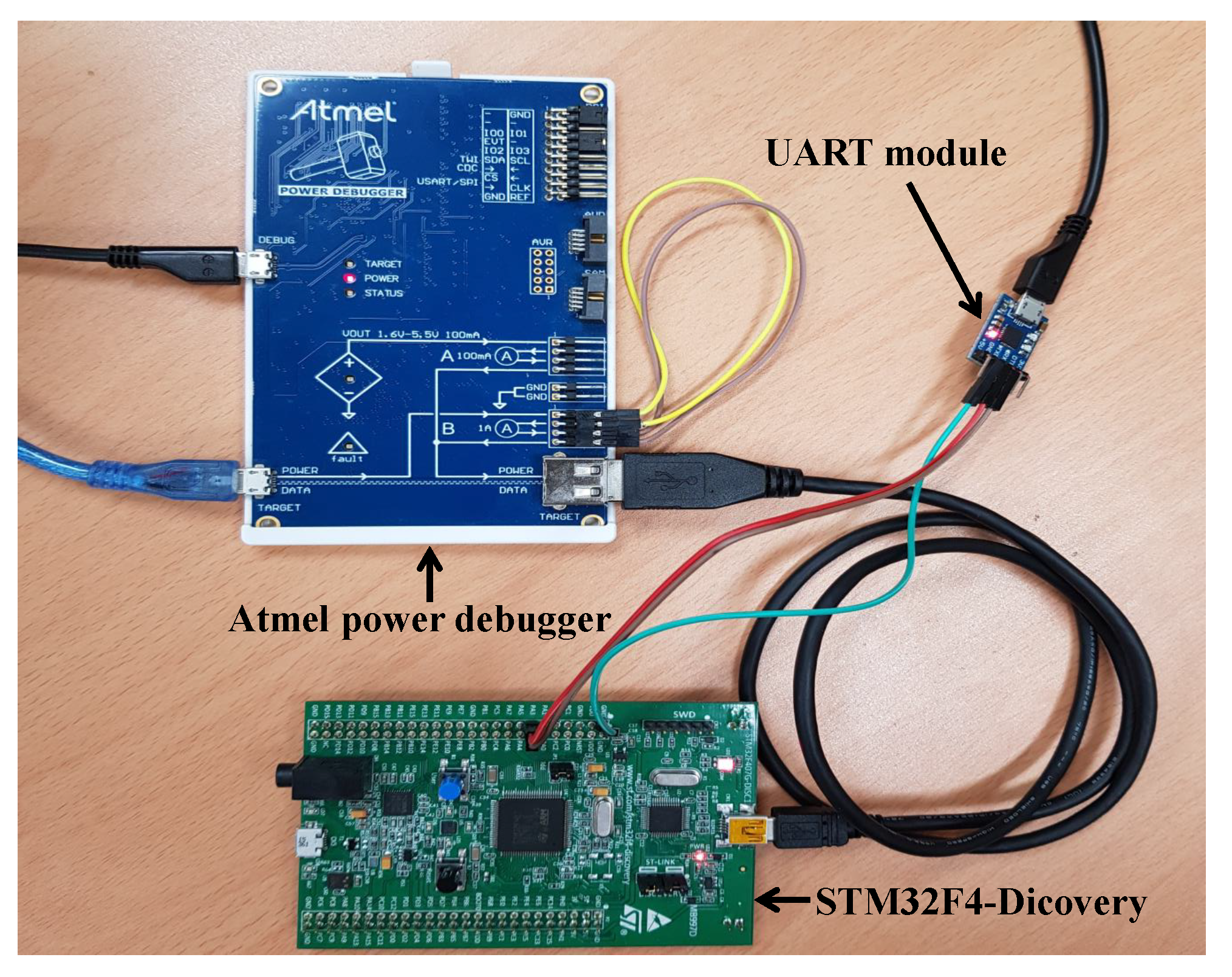
| M | 12 | R | 1 | STM32F4-Discovery | MCU |
| 0 | 12 | UART Module | Data transmission | ||
| 0.2 | Atmel Power Debugger | Power measurement | |||
Publisher’s Note: MDPI stays neutral with regard to jurisdictional claims in published maps and institutional affiliations. |
© 2021 by the authors. Licensee MDPI, Basel, Switzerland. This article is an open access article distributed under the terms and conditions of the Creative Commons Attribution (CC BY) license (http://creativecommons.org/licenses/by/4.0/).
Share and Cite
Oh, S.; Park, D. Low-Power Beam-Switching Technique for Power-Efficient Collaborative IoT Edge Devices. Appl. Sci. 2021, 11, 1608. https://doi.org/10.3390/app11041608
Oh S, Park D. Low-Power Beam-Switching Technique for Power-Efficient Collaborative IoT Edge Devices. Applied Sciences. 2021; 11(4):1608. https://doi.org/10.3390/app11041608
Chicago/Turabian StyleOh, Semyoung, and Daejin Park. 2021. "Low-Power Beam-Switching Technique for Power-Efficient Collaborative IoT Edge Devices" Applied Sciences 11, no. 4: 1608. https://doi.org/10.3390/app11041608