A Study on Deep Learning Application of Vibration Data and Visualization of Defects for Predictive Maintenance of Gravity Acceleration Equipment

Abstract

Hypergravity accelerators are a type of large machinery used for gravity training or medical research. A failure of such large equipment can be a serious problem in terms of safety or costs. This paper proposes a prediction model that can proactively prevent failures that may occur in a hypergravity accelerator. An experiment was conducted to evaluate the performance of the method proposed in this paper. A 4-channel accelerometer was attached to the bearing housing, which is a rotor, and time-amplitude data were obtained from the measured values by sampling. The method proposed in this paper was trained with transfer learning, a deep learning model that replaced the VGG19 model with a Fully Connected Layer (FCL) and Global Average Pooling (GAP) by converting the vibration signal into a short-time Fourier transform (STFT) or Mel-Frequency Cepstral Coefficients (MFCC) spectrogram and converting the input into a 2D image. As a result, the model proposed in this paper has seven times decreased trainable parameters of VGG19, and it is possible to quantify the severity while looking at the defect areas that cannot be seen with 1D.

1. Introduction

All objects on Earth are affected by the Earth’s gravity. Conducting research on microgravity on the ground, instead of outer space, has many practical difficulties. On the other hand, research on hypergravity is relatively easy to carry out using the centrifugal force from a spinning simulation. Hypergravity research requires a gravity simulator that can control gravity by a constant rotation angular speed. Therefore, to conduct hypergravity research, a gravity simulator was developed to enable the formation and maintenance of a hypergravity environment of up to 15 times the Earth’s gravity (15 G), as shown in Figure 1.

Gravitational accelerators are generally used for the hypergravity training of astronauts and can be used for animal testing in basic research for medical purposes. In addition, they can be used to conduct experimental ground tests on the effects of sudden changes in gravity, such as hypergravity and hypogravity, and the changes in pressure that the human body undergoes in a space environment to investigate the biological responses to these harmful stimuli to the human body. These changes in gravity can result in fluid shifts and redistribution in the human body, fluid loss, red blood cell loss, muscle damage, bone damage, hypercalcemia, immune system changes, or spatial disorientation and vertigo [1].

Many studies have examined the changes in the human and animal body due to changes in gravity. The necessity of monitoring the safety and reliability of large gravity acceleration equipment has become an important issue. One of the major issues regarding gravity acceleration equipment is the occurrence of abnormal vibrations when machinery failures occur due to high-speed rotation. The amplification of small vibrations generated in the rotating part of the gravity acceleration equipment may result in damage to the shafts rotating at high speeds, which may lead to serious accidents. Traditional machine learning (ML) that uses feature-based methods [3,4,5] on hand-crafted lists of feature engineering has limitations that cannot improve performance. Furthermore, it is difficult to say that human-designed features are for defective representation. The recently appeared Deep Neural Network (DNN) [6,7,8] has good performance, but it is difficult to describe the characteristics of the defect site due to the parameters of many hidden layers.

This paper proposes a preventive maintenance model that enables the monitoring and visualizing of vibrations that can occur in machinery to proactively prevent the mechanical failures described above.

The remainder of this paper is organized as follows. Section 2 briefly introduces the proposed method and dataset collected from the equipment used in the experiment. In Section 3, we experimented with various models and conditions to evaluate the performance of the proposed model. In addition, we also calculated fault scores through visualizations for each class of faults. Finally, Section 4 proposes a conclusion and future work.

Related Work

Fault Detection using ML: Many studies on vibration-related failures and predictive failure diagnosis have been conducted [3,9,10,11,12,13,14,15,16,17,18,19,20,21]. Lee et al. [3] proposed a rotating mechanism system—a mixture of feature extraction and selection classifies it as a Support Vector Machine (SVM) [4]. Zhang et al. [5] proposed fault detection for bearing wind turbines using ANNs (Artificial Neural Networks). Khlaief et al. [13] adopted a method of learning via K-Nearest Neighbor (KNN), SVM, and Linear Discriminant Analysis (LDA) by screening features based on genetic algorithms to continuously check the state of ball bears in rotating ball bears of asynchronous electrical motors. Le et al. [14] proposed an algorithm based on the ensemble machine learning (EML) for fault detection in Series dc arc and tested its performance using techniques such as bagging, boosting, and stacking various linear classifiers such as fault perceptrons, Decision Trees (DTs), and SVMs. Yang et al. [15] proposed a signal reconstruction modeling technique using support vector regression with a sliding-time-window technique for fault detection. Abdelgayed [16] et al. proposed Decision Tree and K-Nearest Neighbor to diagnose faults in both unlabeled and specified data of transmission and distribution systems with confidence of microgrids. Wang et al. [17] proposed chiller fault detection to enable fast parameter determination without expert assistance using the Bayesian network. Zhang et al. [18] proposed a clustering-based Principal Component Analysis (PCA) to propose a fault detection method for water heat pump systems. Yoo et al. [19] proposed a Fault Detection method using multi-mode PCA and Gaussian mixed model in a sewage heat pump system. Kim et al. [20] proposed the fault detection of photovoltaic current and voltage through the ANN-based modeling method. Zhehan et al. [21] proposed solar current and voltage fault detection using multi-resolution signal composition (MSD) and a two-stage support vector machine classifier.

Fault Detection using Deep Learning (DL): In the case of the CNN (Convolution Neural Network), which is an ANN method, training is carried out using the following procedure: multiple inputs are received; the computation is performed using a model form that the user wants; an output is produced. The method of applying a 1-D CNN model using time-amplitude data with a constant period has been presented as a failure diagnosis method [22,23,24,25,26,27,28,29,30,31]. Another CNN model is 2-D CNN, in which the computation produces images of 3-D shapes with a width and length like the input data as the output [6,32,33,34,35]. There have been many attempts to apply 2-D CNNs to speech recognition and fault diagnosis because 2-D CNNs are transferable with various models [36,37,38,39]. Zong [24] et al. proposed a fault diagnosis of bearing using an autoencoder. Hassan et al. [34] performed fault detection based on acoustic spectral imaging visualizing acoustic emission signals. Shao et al. [25] proposed a fault detection method by constructing feature extractors based on denoising auto-encoder (DAE) and conventional auto-encoder (CAE) for fault detection using vibration data. Shao et al. [26] proposed an autoencoder learning method using an artificial fish swarm algorithm for fault detection of rotating machines. Li et al. [27] proposed a Gaussian–Bernoulli deep Boltzmann machine (GDBM) method for diagnosing rotating machine failures. Sohaib et al. [28] developed a fault-diagnostic system that can overcome axial velocity fluctuations using a deep neural network based on a complex envelope spectra-stacked sparse autoencoder. He et al. [29] presented a fault-finding method based on a Gaussian restricted Boltzmann machine (Gaussian RBM) using envelope spectra of sampled data as a high-dimensional feature vector for fault diagnosis of bearings. Shao et al. [30] proposed a convolutional deep relief network (CDBN) using an expansion moving average (EMA) technique to efficiently learn the fault features of the vibration signal. Verstraete et al. [35] proposed a bearing classification model for a deep learning model after transforming it into a 2D image using short-time Fourier transform, wavelet transform, and Hilbert–Huang transforms. Jiao et al. [31] proposed a one-dimensional CNN-based deep coupled dense convolutional network (CDCN) to integrate information fusion, feature extraction, and fault diagnosis together for intelligent diagnosis.

2. Proposed Method and Environment

The method proposed in this study was divided into three major methods. The first method was to convert vibration data into two-dimensional data by converting time-amplitude data with a constant period, such as the existing signals, into spectrograms. These spectrograms display the time, frequency (Hz), and amplitude, which are used mainly for speech recognition [36,38,39]. The second method was to apply the preprocessed data to a deep neural network model and compare the results with those obtained by the existing machine learning models. Finally, we expressed the fault score and the area representing each class using Class Activation Map (CAM) [40].

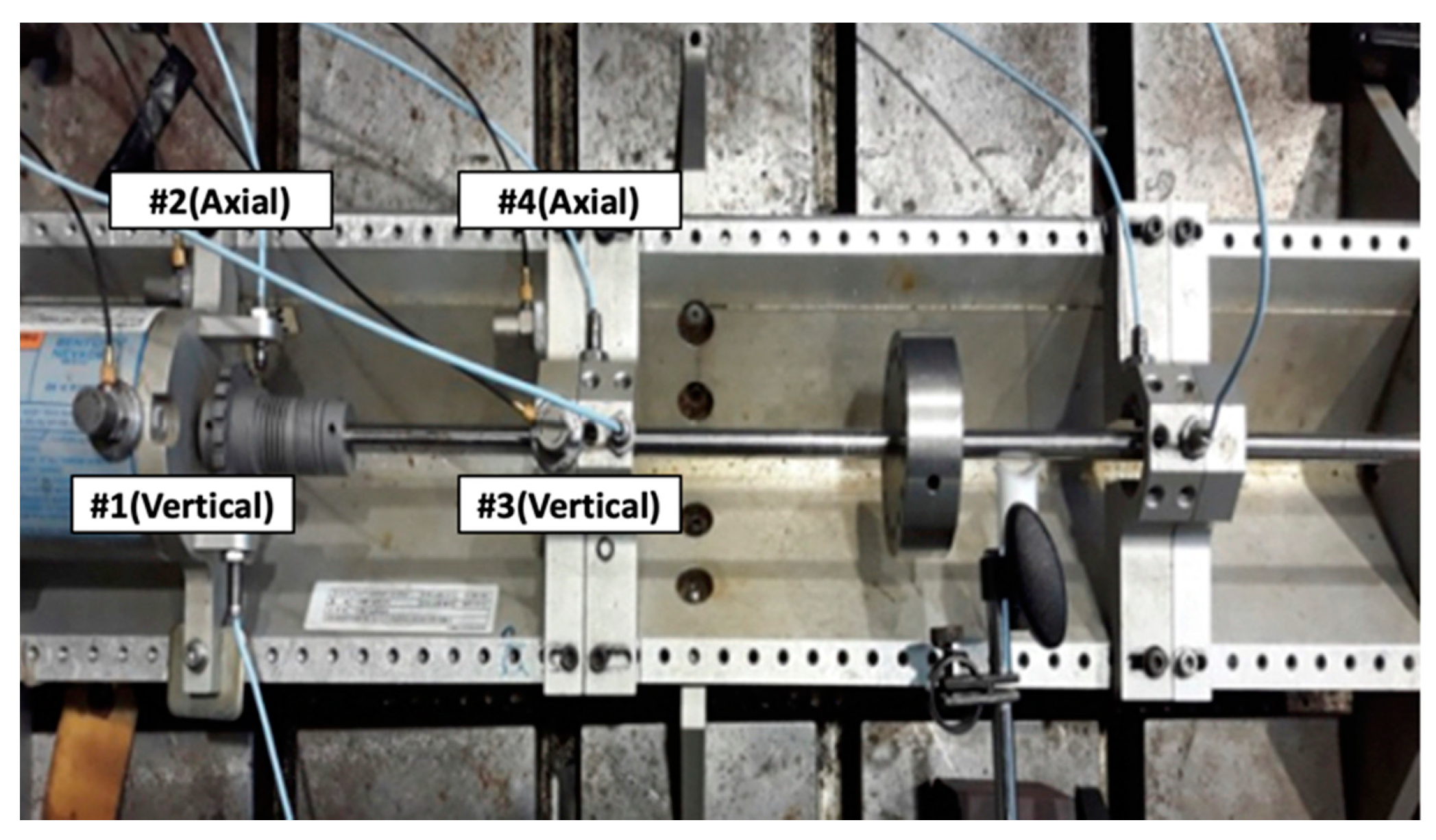
2.1. Design and Fabrication of Experimental Rotating Equipment

The simulation equipment was manufactured as described below. Pulse 3560C and four accelerometers (B&K 4371) were used to acquire the rotation and vibration data, and the data acquisition time for each condition was 30 s.

Table 1. Properties of the data acquisition system [3].

Type	Properties
Pulse 3560C (B&K)	4/2-ch Input/output Module Operating Freq. range: 0~25.6 kHz Direct/Constant Current Line Drive (CCLD)/Microphone (MIC). preamp 1 Tacho Conditioning
Accelerometer (B&K 4371)	Operating Freq. range: 1~25.6 kHz Operating Temp. −50 C~121 C Sensitivity: 9.84 pC/g

lists the specifications of the data acquisition system.

Figure 2 presents the RK4 (Rotor-kit) of the lab-scale rotating simulation equipment, which is the experimental model, and the locations of the sensors used in the experiment. The experiment system was composed of a motor to operate the rotating equipment, a flexible coupling connecting the rotor and motor, and two copper sleeve bearings supporting the rotor. An 800 g disk was installed between the bearings to simulate the unbalance fault. Sensors were installed on the drive-end side of the motor and rotor. The measurements were taken at locations in the vertical and axial directions of the motor and rotor. The experimental equipment was operated at 2000 RPM (Rotating Per Minute), avoiding 2400 RPM, which is the first critical speed.

In this experiment, fault simulations were carried out by simulating four representative conditions of the rotating equipment: Normal, Unbalance, Misalignment, and Shaft rubbing conditions. Figure 3 presents the methods of application of the normal condition and each type of fault. A normal condition was obtained after performing shaft balancing using the RK4, and the residual unbalance was measured to be 0.02 g/117.4° after balancing. Unbalance was induced by attaching a 3.2 g object in a direction towards the location of residual unbalance (117.4°). Misalignment was achieved by installing a 4 mm shim plate at the foot of the drive-end side of the motor, and shaft rubbing was applied in the horizontal direction using a magnetic base. In addition, a contact device made from Teflon was used to minimize the damage to the axis that may occur due to rubbing.

Unbalance is the most fundamental fault that causes vibrations in rotating equipment. Unbalance occurs when the mass distribution of the rotor is asymmetric with respect to the axis centerline, and all the causes of unbalance exist to some degree in the rotors. Excessive unbalance increases the vibrations and noise of the rotating equipment. As a result, fatigue destruction may occur due to a deterioration of the bearings and consumable parts.

Misalignment is one of the most common faults of rotating equipment along with unbalancing [41], and refers to a condition where the centers of the two axes do not coincide, or a condition where the centers coincide but are not parallel. A large degree of misalignment can cause overheating of the coupling, an increase in the shaft cracks and fatigue, and damage to the bearings and consumable parts.

A rubbing fault is a secondary transient phenomenon caused by excessive unbalance and misalignment in rotating machinery [42]. Rubbing may be caused by the occurrence of friction between the stator and rotor caused by excessive vibrations, or a narrow gap due to thermal expansion during equipment operation. Continuous rubbing during the operation of rotating machinery may cause the separation of parts or axis bending, and severe rubbing can lead to the destruction of the rotating equipment.

The sampling rate of the obtained signals was 65,536 Hz. The signals measured for 30 s were divided into 0.48-s units considering the measurement environment of the actual equipment, and each of the 0.48-s units was assumed to be one dataset. Machine learning was performed by dividing one dataset into 14 samples. Sampling was performed because a vibration is a periodic signal in the time domain [43], and most fault signals have periodicity. Therefore, sampling is used to examine the consistency and continuity of each condition using the features calculated from the signals.

The signal segmentation for sampling was based on the rotational frequency of the rotor. Generally, in rotating equipment, the rotational frequency is the most dominant component, and the majority of fault components appear in the harmonic form of the rotational frequency. Therefore, the length of the sample of experimental data was set to 0.06 s. This was two times 0.03 s, which is the period of vibrations at 2000 RPM, and the number of samples was increased by overlapping half the signal.

The total number of training and test data was 1056, and the dataset was divided into training and testing datasets by allocating 80% to the training dataset and 20% to the testing dataset. At this time, the training dataset consisted of 229 Normal condition data (no faults in operation), 199 Rubbing data, 205 Unbalance data, and 211 Misalignment data, and the testing dataset included 43 Normal data, 61 Rubbing data, 55 Unbalance data, and 53 Misalignment data.

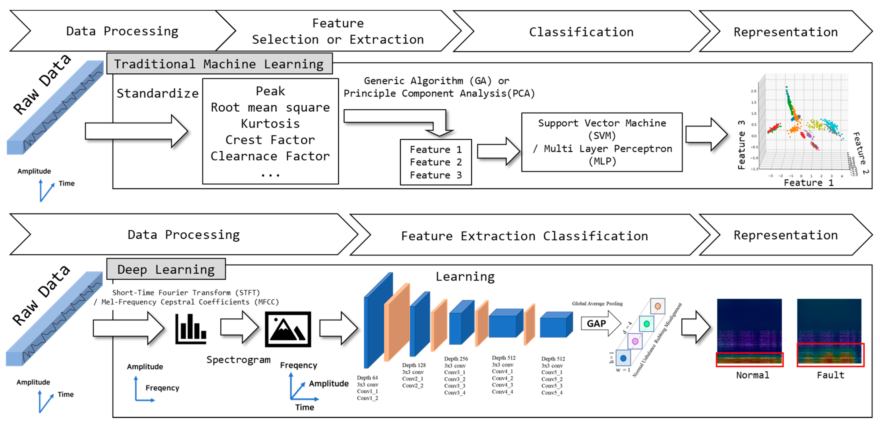
2.2. Proposed Method

Figure 4 is a comparison between the proposed deep method and machine learning. Data are acquired from the laboratory equipment at 0.06 s intervals as shown in Section 2.1. Traditional machine learning selects features hand-crafted by someone with knowledge of the vibration anomaly detection domain. For better visualization or classification, the feature is reduced in dimension and then an algorithm such as SVM or Multi-Layer Perceptron (MLP) is applied. After that, the cause analysis is performed through visualization, where the characteristics are located for each datum.

The proposed method uses a spectrogram to visualize the processing of signals from each class of Short-Time Fourier Transform (STFT) or Mel Frequency Cepstral Coefficients (MFCC) signals, such as in Figure 5. Applying a spectrogram changes the existing one-dimensional input into two dimensions. A two-dimensional based deep learning model is learned through transfer learning. After that, the CAM is applied to calculate and visualize the fault score through differences from the defect class except for the normal, and the cause analysis for each class can be visualized and quantified.

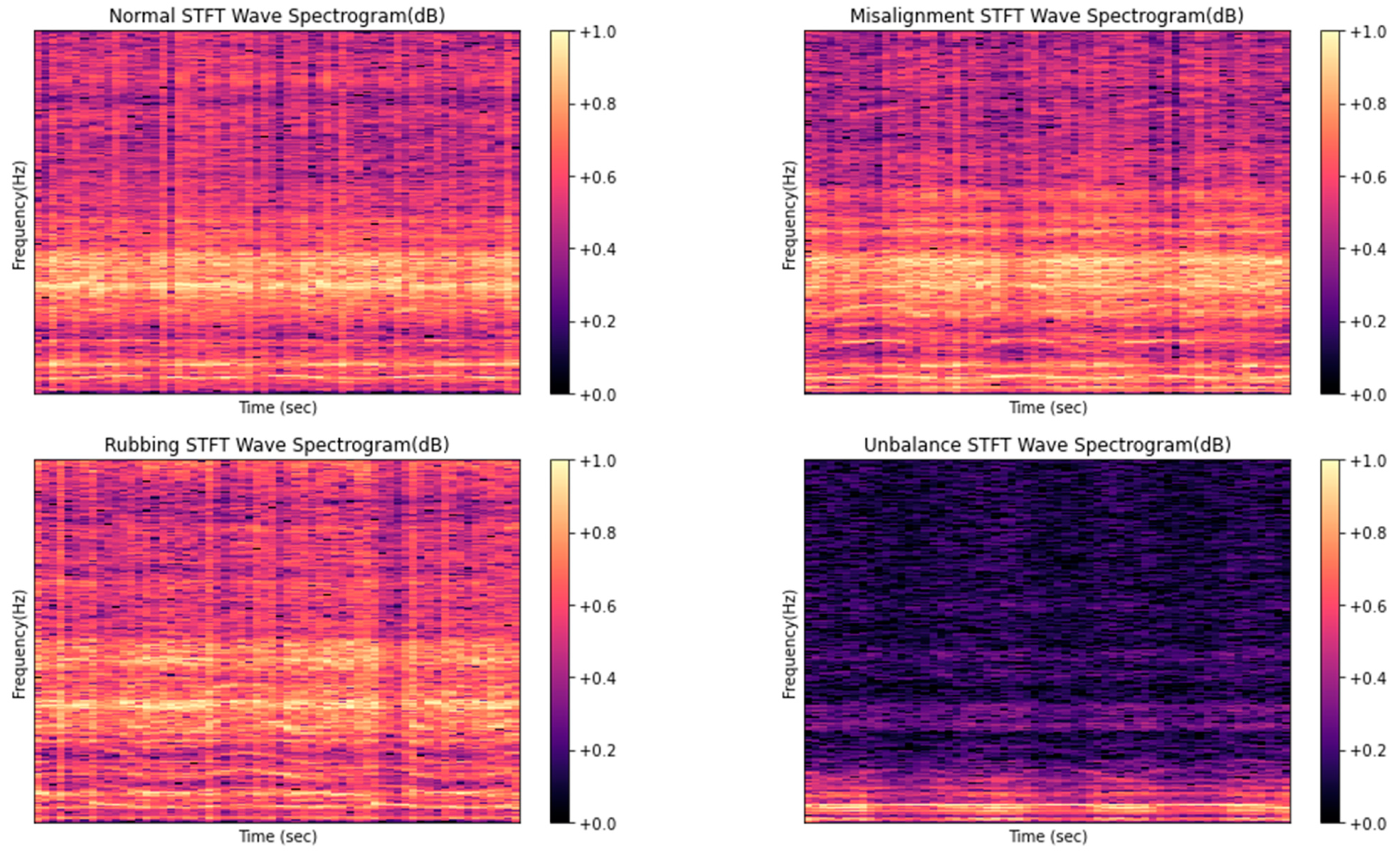
2.2.1. STFT (Short-Time Fourier Transform)

With respect to the method for converting time-amplitude data to 2D images, spectrograms were used after performing discrete STFT. Discrete STFT is a method of partitioning continuous signals over a long period into shorter segments at short time intervals and applying a Fourier transform to each signal segment. This technique allows researchers to observe how the vibrations of signals change with time. These changes in vibrations can be expressed as Equation (1) [44,45]:

$$X\left(k,n\right)={\displaystyle \sum }_{m=0}^{L-1}w\left[m\right]x\left[m+nH\right]exp\left(-2\pi k/N\right)m$$

(1)

$w\left[m\right]$ was assumed to be a non-zero window function in the interval $m=0,1,\cdot \cdot \cdot ,L-1$, and $L$ is the window length, and a smaller signal than the signal $x\left[m\right]$. In this experiment, the Han window was applied as the window function [45]. $w\left[m\right]x\left[n+nH\right]$ is a non-zero signal in $m=0,1,\dots ,L-1$. The signal $x\left[m\right]$ is a form that undergoes $N$ point DFT (Discrete Fourier Transform) according to the hop size of $H$(=512). The hop size H is specified in samples and determines the step size moving through the window in the overall signal [45]. Therefore, FFT was calculated according to the size of $m$. Because a signal generated through this process constitutes a different spectrum with time, it cannot be represented as a spectrum. Therefore, it was represented by taking $\left|X\left(k,n\right)\right|$ and applying a color map (spectrogram), as shown in Figure 6.

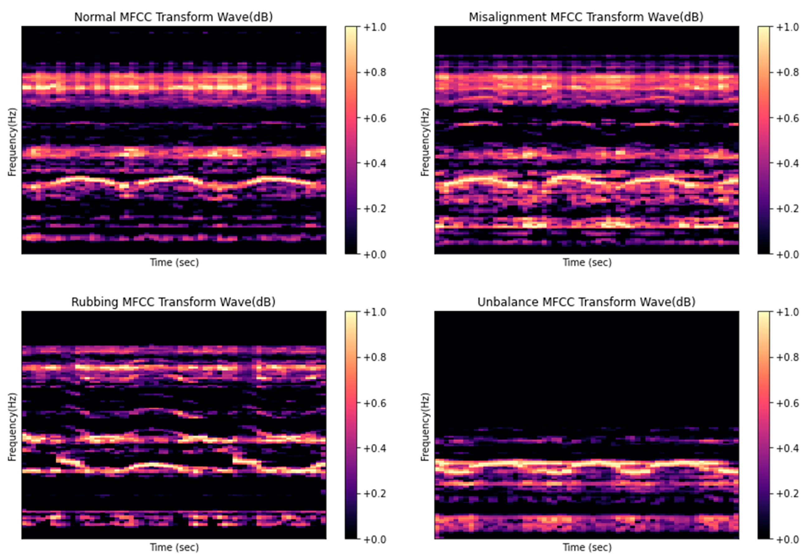
2.2.2. MFCCs (Mel Frequency Cepstral Coefficients)

MFCC is a conversion algorithm used mainly in speech recognition. This is one of the methods for extracting the features from sound signals, and the procedure for feature extraction consists of the following six steps [38,39], as shown in Figure 7:

• Frame the signal into short frames.
• For each frame, calculate the periodogram estimate of the power spectrum.
• Apply the mel filterbank to the power spectra, and sum the energy in each filter.
• Take the logarithm of all filterbank energies.
• Take the Discrete Cosine Transform (DCT) of the log filterbank energies.
• Keep DCT coefficients 2–13, and discard the rest.

2.3. Deep Learning Network

The deep learning neural network architecture proposed in this study was based on VGG19 [6]. VGG19 is a model that is widely used as a basic deep learning method because it is relatively easy to implement and modify because it uses only 3 × 3 convolutional layers. In this study, the number of parameters was reduced using Global Average Pooling (GAP) to eliminate the Fully Connected Layer (FCL), which is one of the parts of VGG19 that requires a large number of computations, and to match with the output layer. The deep learning architecture was constructed, as shown in Figure 4 (Down).

The size of the spectrogram images in Figure 6 and Figure 7 used as training data was changed by converting a rectangular shape (432, 288) to a square shape (298, 298) before using it in the experiment. For convergence of the learning errors, an attempt was made to find the global minimum error using the learning scheduler [5], which changes the learning rate each epoch. The other hyperparameters were set, as shown in

Table 2. Hyperparameters used in model training.

Hyper Parameter	Value
Learning Rate	0.001
Batch Size	4
Warm-up Train phase	10
Weight Decay	0.0001
Optimizer	SGD (Stochastic Gradient Descent)
Epoch	200
Early Stopping patience	10

.

An initial learning rate of 0.001 was set for faster training speeds. A batch size of four was used to set the maximum batch size in the environment to speed up learning. The early 10 epochs were used to warm-up [46] the training phase and adjust the learning rate according to the complexity of the training data. The first 200 epochs were used for a more robust model. Lastly, to avoid overfitting, an early stopping [47] technique was introduced based on the verification data, and the patience was set to 10.

2.4. Fault Score

In this paper, the Global Average Pooling (GAP) layer was applied later to calculate and visualize the fault score using CAM. In general, the Fully Connected Layer (FCL) has the disadvantage of losing feature map location information through CNN. This was applied as GAP, and using CAM, it is possible to check the characteristics of which part of the image the deep learning model looked at and determined the class. The equation process for deriving the CAM to be used in this paper can be derived by Equation (2):

$$\begin{array}{c}{S}_c={\displaystyle {\displaystyle \sum }_k}{w}_k^c{F}_k\\ ={\displaystyle {\displaystyle \sum }_k}{w}_c^k{\displaystyle {\displaystyle \sum }_{x,y}}{f}_k\left(x,y\right)\\ ={\displaystyle {\displaystyle \sum }_{x,y}}{\displaystyle {\displaystyle \sum }_k}{w}_k^c{f}_k\left(x,y\right)\end{array}$$

(2)

As seen in Equation (2), given an image, let $f_k\left(x,y\right)$ be a feature map located at $\left(x,y\right)$ through the last $k$ convolution layers. When we obtain the value for all the features, it becomes $F_k$, and the sum of the probability $w$ obtained for a specific class $c$ is called Class Score $S_c$. In other words, the larger $w_c^k$ is, the greater the influence of $F_k$ in class $c$.

$$FaultScore={\displaystyle \sum }_{x,y}\left|{\displaystyle \sum }_i^N\frac{S\left(X_i\right)}{N}-S\left(\widehat{X}\right)\right|$$

(3)

Equation (3) is the failure score proposed in this paper. For the $N$ training normal images $X$, the CAM was calculated using the absolute value of the difference with the CAM result of $\widehat{X}$. Each image has the same number of $x,y$ pixels.

2.5. Deep Learning Environment

In this study, the deep learning environment for training and testing a deep learning model was built with a PC with the following configuration: 32 GB Random Access Memory (RAM), i5-8500 3.0 GHz Central Processing Unit (CPU), and RTX 2080 Ti Graphics Processing Unit (GPU). The experimental software environment was developed in a Python 3.7.6 environment, and the main packages used to set up the environment were Pytorch 1.5 [43], librosa 0.6.3 [48], and sklearn 0.22 [49].

3. Experiment Result

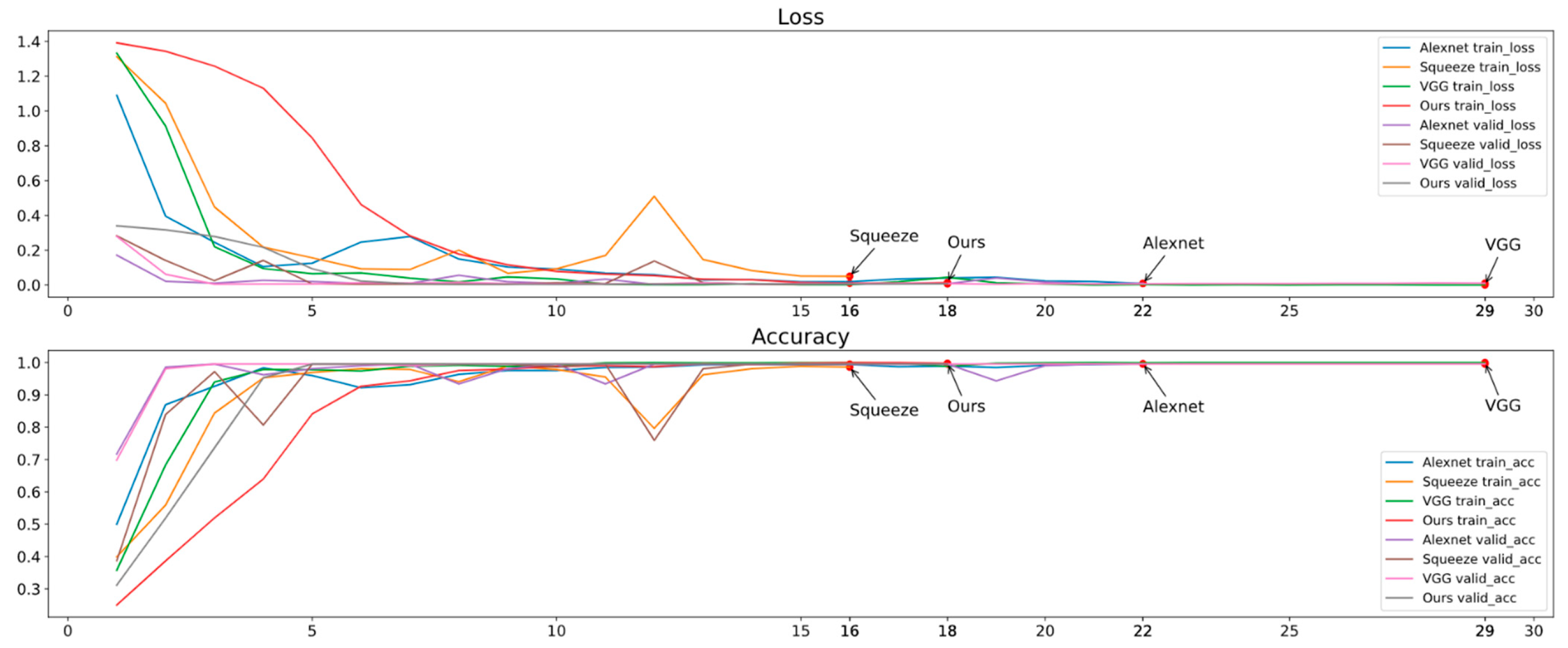
3.1. Performance Evaluation

In the experiments of this study, the accuracy, precision, recall, and F1-Score were measured using True Positive (TP), True Negative (TN), False Positive (FP), and False Negative (FN). The accuracy, precision, recall, and F1 Score can be expressed using Equations (4)–(7), respectively.

$$Accuracy=\frac{TP+TN}{TP+TN+FP+FN}$$

(4)

$$Precision=\frac{TP}{TP+FP}$$

(5)

$$Recall=\frac{TP}{TP+FN}$$

(6)

$$F_{1}Score=2\times \frac{\mathit{Precision}\times \mathit{Recall}}{\mathit{Precision}+\mathit{Recall}}$$

(7)

At this time, to demonstrate the superiority of the methods used in this experiment, they were compared with one of the most commonly used methods, the method of applying SVM (Support Vector Machine), after feature selection based on the GA (genetic algorithm) after extracting the hand-crafted features from a raw signal and [3]. The [3] method is a method of applying SVM by mixing a GA and PCA (Principal Component Analysis) from a list of hand-crafted feature values through feature engineering. The proposed methods were also compared with the MLP (Multi-Layer Perceptron) method [5] from the same feature engineering [3] to determine if it shows better performance in training after data visualization.

Table 3. Experimental Results.

Class	Model	Accuracy	Precision	Recall	F1
Normal	STFT based + our model	0.98	1.0	0.98	0.99
	MFCC based + our model	0.98	1.0	0.98	0.99
Rubbing	STFT based + our model	1.0	1.0	1.0	1.0
	MFCC based + our model	1.0	1.0	1.0	1.0
Unbalance	STFT based + our model	1.0	0.98	1.0	0.99
	MFCC based + our model	1.0	0.98	1.0	0.99
Misalignment	STFT based + our model	1.0	1.0	1.0	1.0
	MFCC based + our model	1.0	1.0	1.0	1.0

lists the experimental results. Under Normal, Rubbing, Unbalance, and Misalignment conditions, the proposed methods showed better performance than the existing methods [3,5]. In this study, an attempt was made to improve performance through k-fold cross-validation, but the following problems were encountered. First, the accuracy was low compared to the results not applied because the number of datasets was not large. Second, the experimental results of the current dataset were not applied because they were unnecessary owing to the very high accuracy.

The performance of the deep learning methods was superior to that of a method based on MLP or SVM, as listed in Table 3. This can be attributed to a large amount of information that cannot be expressed as features that are lost when selecting the features of input data in the preprocessing stage. Although all hand-crafted features were selected and learned using the MLP algorithm, a performance equal to or better than that of deep learning could not be achieved. As shown in the results in Table 3, the results of our DNN models using two methods transforming raw data into images through STFT and MFCC were almost identical. Any preprocessing method such as STFT or MFCC doesn’t impact to extracting semantic information from CNN filters and output metric of the DNN model.

Table 4. Train noise-added data to compare test results with existing deep learning models.

Method	Algorithm	Parameters	Accuracy	Precision	Recall	F1
Machine Learning	MLP [5]	74,500	0.95	0.9525	0.955	0.9525
	GA-SVM [3]	-	0.51	0.507	0.505	0.5025
	PCA-SVM [3]	-	0.96	0.9625	0.9675	0.965
Deep Learning	Squeeze Net [8]	737,476	0.995	0.982	0.985	0.985
	Alex Net [7]	57,020,228	0.995	0.995	0.995	0.995
	VGG19 [6]	139,597,636	0.995	0.995	0.995	0.995
	Our	20,037,444	0.995	0.995	0.995	0.995

compares the training results based on the dataset that has undergone an STFT transformation with the existing deep learning model [6,7,8,33]. The training hyperparameters of each model were trained under the same conditions, as listed in Table 2. Table 4 shows that DNN is superior to traditional machine learning models with hand crafted characteristics. In addition, in the case of the proposed model, the number of SqueezeNet parameters was large, but the performance of Equations (4)-(7) was excellent. Also, if we compare our method with two Alex Net and VGG19, the performance of the equations are the same but the parameters are much lower than others. As a result, it was confirmed that the proposed model works well with GAP without the existing FCL.

In Figure 8, the left figure compares Validation Loss and Train Loss, and the right figure compares Train Accuracy and Validation Accuracy. Each model is all finished before the epochs set before running out due to Early Stopping. Experiments have confirmed that the model proposed in this paper shows better accuracy than the comparison model in

Table 5. Results of the models proposed in this paper and existing deep learning models learned based on data with noise.

	Transfer Learning	Epoch	Train Accuracy	Train Loss	Valid Accuracy	Valid Loss
Ours	Yes	23	0.991	0.033	0.995	0.007
	No	22	0.988	0.050	0.995	0.009
Squeeze Net [8]	Yes	22	0.990	0.066	0.995	0.004
	No	114	0.760	0.364	0.707	0.107
AlexNet [7]	Yes	22	0.986	0.053	0.995	0.007
	No	12	0.271	1.385	0.203	0.348
VGG19 [6]	Yes	16	0.982	0.062	0.995	0.008
	No	17	0.985	0.043	0.995	0.004

. Although the VGG19 [6]-based model proposed in this paper ended later than SqueezeNet, it was confirmed that it is superior in terms of loss and acceleration stability. Table 5 is a representation of the results of Figure 8, which is the result of training the proposed deep learning model and the existing deep learning models by adding noise to the data. As shown in Table 5, Transfer Learning was concluded to help produce more robust results. We confirm that the model proposed in this paper has the least learning accuracy and learning loss, and the least validation loss compared to VGG19.

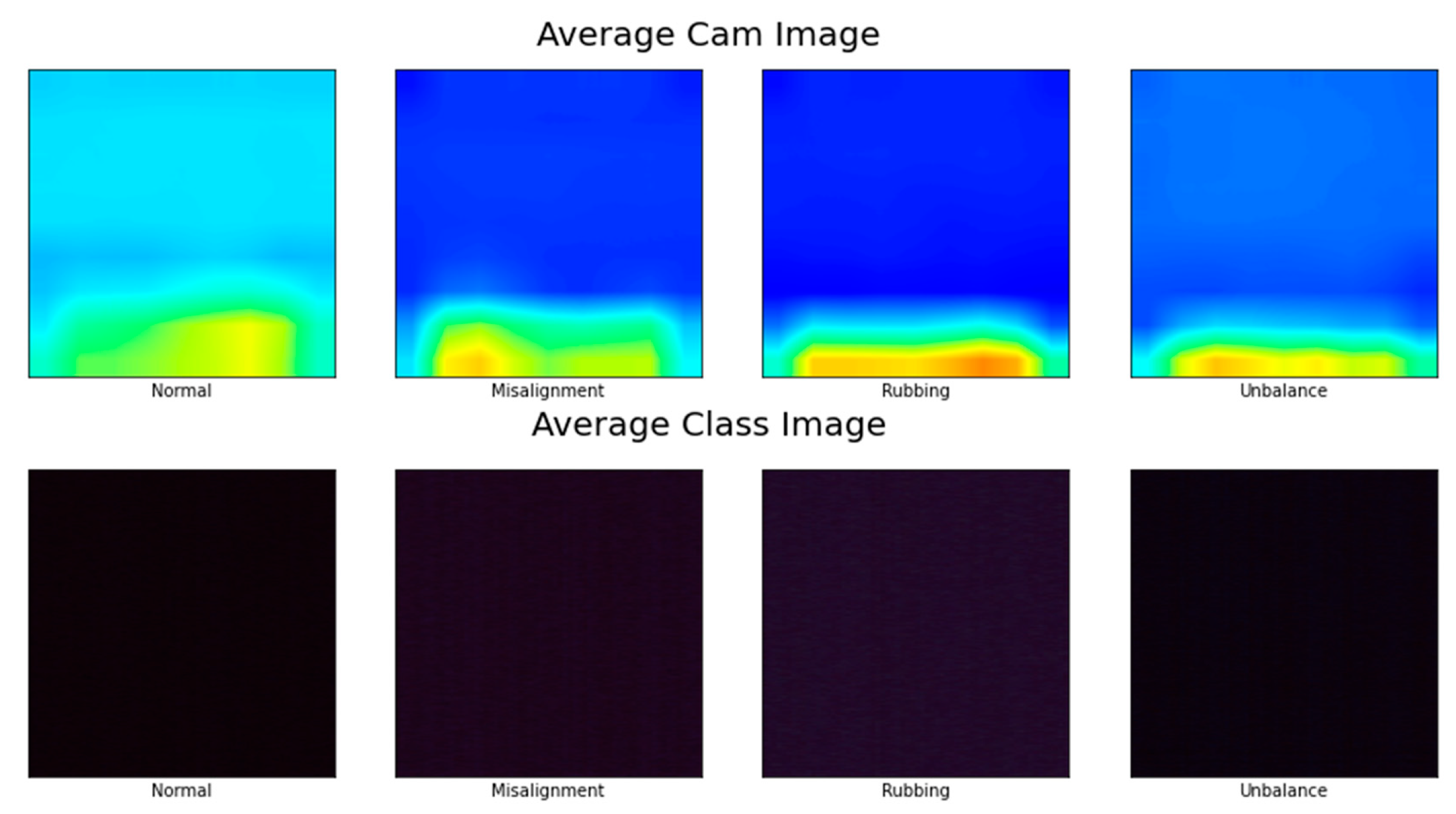
3.2. Visualization of Failure Causes

Figure 9 shows the CAM result (Up) of the test data and the average value (Down) of the input image as the proposed method. It is difficult for a human to identify an abnormal image in the average class image. However, when looking at the result of CAM, the difference between the normal class and other defect classes is clearly visible.

In Figure 10, there is a lot of change compared to Figure 9 because there is noise in the data.

3.3. Fault Score Variation

The Fault Score proposed in this paper has a distribution as shown in Figure 11. Because the Normal class is the standard label, the Failure Score is averagely small, about Normal (0.2), and the highest class is Rubbing (0.8), and it is composed in the order of Misalignment (0.7) and Unbalance (0.5). We can identify the normality and abnormality of the image class depending on the value of the fault score. Each defect class has the same minimum and maximum values as the Normal condition class. The disappearance of locality caused by adding the score shows this result.

4. Conclusions and Future Work

The vibration signals were measured with accelerometers to prevent accidents that can occur in large equipment, such as a gravitational accelerator. In this paper, four signals that can arise when a defect occurs in the rotating part of a gravitational accelerometer were analyzed. The existing vibration data can also be converted into image data, such as spectrograms, which are mainly used in speech recognition, and they can also be applied to an image-based deep learning model. The measured data were used to train and test a deep learning model using the spectrogram visualization based on the MFCC and STFT, and the proposed method was evaluated.

The major methods used in this experiment were to convert vibration signals to images and apply a modified DNN model to a fault model. The proposed deep learning architecture enabled a diagnosis of the four conditions, such as Normal, Rubbing, Misalignment, and Unbalance. Both MFCC and STFT models showed an average accuracy of 99.5%. According to the experiment, there was no difference in performance due to processing between STFT and MFCC in the four classifications of vibration data. In addition, the proposed model was compared with GA-SVM, PCA-SVM, and MLP, which are machine learning models made with hand-crafted features. The experimental results showed that the proposed models have better performance in terms of accuracy, recall, precision, and F1-Score compared to hand-crafted feature-based models. So, performance, accuracy, and learning speed were compared with the existing deep learning method. These results suggest that the proposed method can be used successfully as a fault diagnosis and assessment model if the monitoring environment is constructed by attaching sensors in an assessment of the stability of gravity acceleration equipment in the future. In addition, it was confirmed that VGG19, which replaced FCL with GAP, works well for vibration data learning to be applied in this paper. In comparison with the deep learning model, it was confirmed that the parameter was reduced by about seven times compared to the existing VGG19 because there was no FCL. As the data to be applied in this paper, the performance of the proposed deep learning model was almost similar, which was confirmed by Early Stopping that the complexity of the data is higher than that of the model.

Finally, using CAM, it was possible to measure abnormal areas of data that humans cannot see, and a failure score to quantify this was proposed. The Failure Score proposed in this paper can act as a measure to check how much difference there is compared to the Normal class. The proposed method can show the area of the defect. This is possible because the one-dimensional signal is expanded in two dimensions. Based on the characteristics of signal, which is periodic difference between each class, we applied CAM and proposed a fault score.

The method proposed in this study had the following limitations. The patterns of the fault data need to be prepared in advance. It is believed to bring high accuracy because the data complexity is lower than that of the model. This is believed to be because it is a repetitive signal due to the nature of vibration data. Second, training takes considerable time and requires additional hardware, such as GPUs. Considering these limitations, a method that can reduce the computation cost so that the proposed method can be used in small edge devices will be needed before this method can be commercialized.

References

1. Gurovsky, N.N.; Gazenko, O.G.; Adamovich, B.A.; Ilyin, E.A.; Genin, A.M.; Korolkov, V.I.; Shipov, A.A.; Kotovskaya, A.R.; Kondratyeva, V.A.; Serova, L.V.; et al. Study of physiological effects of weightlessness and artificial gravity in the flight of the biosatellite Cosmos-936. Acta Astronaut. 1980, 7, 113–121. [Google Scholar] [CrossRef]
2. Jang, T.Y.; Kim, K.-S.; Kim, Y.H. Altered Gravity and Immune Response. Korean J. Aerosp. Environ. Med. 2018, 28, 6–8. [Google Scholar]
3. Lee, W.-K.; Cheong, D.-Y.; Park, D.-H.; Choi, B.-K. Performance Improvement of Feature-Based Fault Classification for Rotor System. Int. J. Precis. Eng. Manuf. 2020, 21, 1065–1074. [Google Scholar] [CrossRef]
4. Aydmj, T.; Duin, R.P.W. Pump Failure Determination Using Support Vector Data Description; Lecture Notes in Computer Science; Springer: Berlin/Heidelberg, Germany, 1999; pp. 415–425. [Google Scholar]
5. Zhang, Z.-Y.; Wang, K.-S. Wind turbine fault detection based on SCADA data analysis using ANN. Adv. Manuf. 2014, 2, 70–78. [Google Scholar] [CrossRef] [Green Version]
6. Simonyan, K.; Zisserman, A. Very deep convolutional networks for large-scale image recognition. arXiv 2014, arXiv:1409.1556. [Google Scholar]
7. Krizhevsky, A.; Sutskever, I.; Hinton, G.E. Imagenet classification with deep convolutional neural networks. Adv. Neural Inf. Process. Syst. 2012, 25, 1097–1105. [Google Scholar] [CrossRef]
8. Iandola, F.N.; Han, S.; Moskewicz, M.W.; Ashraf, K.; Dally, W.J.; Keutzer, K. SqueezeNet: AlexNet-level accuracy with 50x fewer parameters and <0.5 MB model size. arXiv 2016, arXiv:1602.07360. [Google Scholar]
9. Riaz, S.; Elahi, H.; Javaid, K.; Shahzad, T. Vibration feature extraction and analysis for fault diagnosis of rotating machinery-a literature survey. Asia Pac. J. Multidiscip. Res. 2017, 5, 103–110. [Google Scholar]
10. Mellit, A.; Tina, G.M.; Kalogirou, S.A. Fault detection and diagnosis methods for photovoltaic systems: A review. Renew. Sustain. Energy Rev. 2018, 91, 1–17. [Google Scholar] [CrossRef]
11. Liu, R.; Yang, B.; Zio, E.; Chen, X. Artificial intelligence for fault diagnosis of rotating machinery: A review. Mech. Syst. Signal Process. 2018, 108, 33–47. [Google Scholar] [CrossRef]
12. Song, L.; Wang, H.; Chen, P. Vibration-based intelligent fault diagnosis for roller bearings in low-speed rotating machinery. IEEE Trans. Instrum. Meas. 2018, 67, 1887–1899. [Google Scholar] [CrossRef]
13. Khlaief, A.; Nguyen, K.; Medjaher, K.; Picot, A.; Maussion, P.; Tobon, D.; Chauchat, B.; Cheron, R. Feature engineering for ball bearing combined-fault detection and diagnostic. In Proceedings of the 2019 IEEE 12th International Symposium on Diagnostics for Electrical Machines, Power Electronics and Drives (SDEMPED), Toulouse, France, 27–30 August 2019; IEEE: Piscataway, NJ, USA, 2019; pp. 384–390. [Google Scholar]
14. Le, V.; Yao, X.; Miller, C.; Tsao, B.-H. Series dc arc fault detection based on ensemble machine learning. IEEE Trans. Power Electron. 2020, 35, 7826–7839. [Google Scholar] [CrossRef]
15. Yang, C.; Liu, J.; Zeng, Y.; Xie, G. Real-time condition monitoring and fault detection of components based on machine-learning reconstruction model. Renew. Energy 2019, 133, 433–441. [Google Scholar] [CrossRef]
16. Abdelgayed, T.S.; Morsi, W.G.; Sidhu, T.S. Fault detection and classification based on co-training of semisupervised machine learning. IEEE Trans. Ind. Electron. 2017, 65, 1595–1605. [Google Scholar] [CrossRef]
17. Wang, Y.; Wang, Z.; He, S.; Wang, Z. A practical chiller fault diagnosis method based on discrete Bayesian network. Int. J. Refrig. 2019, 102, 159–167. [Google Scholar] [CrossRef]
18. Zhang, H.; Chen, H.; Guo, Y.; Wang, J.; Li, G.; Shen, L. Sensor fault detection and diagnosis for a water source heat pump air-conditioning system based on PCA and preprocessed by combined clustering. Appl. Therm. Eng. 2019, 160, 114098. [Google Scholar] [CrossRef]
19. Yoo, Y.-J. Fault Detection Method Using Multi-mode Principal Component Analysis Based on Gaussian Mixture Model for Sewage Source Heat Pump System. Int. J. Control Autom. Syst. 2019, 17, 2125–2134. [Google Scholar] [CrossRef]
20. Kim, I.-S. On-line fault detection algorithm of a photovoltaic system using wavelet transform. Sol. Energy 2016, 126, 137–145. [Google Scholar] [CrossRef]
21. Yi, Z.; Etemadi, A.H. Line-to-line fault detection for photovoltaic arrays based on multiresolution signal decomposition and two-stage support vector machine. IEEE Trans. Ind. Electron. 2017, 64, 8546–8556. [Google Scholar] [CrossRef]
22. Ince, T.; Kiranyaz, S.; Eren, L.; Askar, M.; Gabbouj, M. Real-time motor fault detection by 1-D convolutional neural networks. IEEE Trans. Ind. Electron. 2016, 63, 7067–7075. [Google Scholar] [CrossRef]
23. Eren, L. Bearing fault detection by one-dimensional convolutional neural networks. Math. Probl. Eng. 2017, 2017. [Google Scholar] [CrossRef] [Green Version]
24. Meng, Z.; Zhan, X.; Li, J.; Pan, Z. An enhancement denoising autoencoder for rolling bearing fault diagnosis. Measurement 2018, 130, 448–454. [Google Scholar] [CrossRef] [Green Version]
25. Shao, H.; Jiang, H.; Zhao, H.; Wang, F. A novel deep autoencoder feature learning method for rotating machinery fault diagnosis. Mech. Syst. Signal Process. 2017, 95, 187–204. [Google Scholar] [CrossRef]
26. Shao, H.; Jiang, H.; Wang, F.; Zhao, H. An enhancement deep feature fusion method for rotating machinery fault diagnosis. Knowl. Based Syst. 2017, 119, 200–220. [Google Scholar] [CrossRef]
27. Li, C.; Sánchez, R.-V.; Zurita, G.; Cerrada, M.; Cabrera, D. Fault diagnosis for rotating machinery using vibration measurement deep statistical feature learning. Sensors 2016, 16, 895. [Google Scholar] [CrossRef] [PubMed] [Green Version]
28. Sohaib, M.; Kim, J.-M. Reliable fault diagnosis of rotary machine bearings using a stacked sparse autoencoder-based deep neural network. Shock Vib. 2018, 2018, 2919637. [Google Scholar] [CrossRef] [Green Version]
29. He, X.; Wang, D.; Li, Y.; Zhou, C. A novel bearing fault diagnosis method based on gaussian restricted boltzmann machine. Math. Probl. Eng. 2016, 2016, 2957083. [Google Scholar] [CrossRef]
30. Shao, H.; Jiang, H.; Zhang, H.; Duan, W.; Liang, T.; Wu, S. Rolling bearing fault feature learning using improved convolutional deep belief network with compressed sensing. Mech. Syst. Signal Process. 2018, 100, 743–765. [Google Scholar] [CrossRef]
31. Jiao, J.; Zhao, M.; Lin, J.; Ding, C. Deep coupled dense convolutional network with complementary data for intelligent fault diagnosis. IEEE Trans. Ind. Electron. 2019, 66, 9858–9867. [Google Scholar] [CrossRef]
32. Szegedy, C.; Liu, W.; Jia, Y.; Sermanet, P.; Reed, S.; Anguelov, D.; Erhan, D.; Vanhoucke, V.; Rabinovich, A. Going deeper with convolutions. In Proceedings of the IEEE Conference on Computer Vision and Pattern Recognition, Boston, MA, USA, 7–12 June 2015; pp. 1–9. [Google Scholar]
33. He, K.; Zhang, X.; Ren, S.; Sun, J. Deep residual learning for image recognition. In Proceedings of the IEEE Conference on Computer Vision and Pattern Recognition, Las Vegas, NV, USA, 27–30 June 2016; pp. 770–778. [Google Scholar]
34. Hasan, M.J.; Islam, M.M.; Kim, J.-M. Acoustic spectral imaging and transfer learning for reliable bearing fault diagnosis under variable speed conditions. Measurement 2019, 138, 620–631. [Google Scholar] [CrossRef]
35. Verstraete, D.; Ferrada, A.; Droguett, E.L.; Meruane, V.; Modarres, M. Deep learning enabled fault diagnosis using time-frequency image analysis of rolling element bearings. Shock Vib. 2017, 2017, 5067651. [Google Scholar] [CrossRef]
36. Salamon, J.; Bello, J.P. Deep convolutional neural networks and data augmentation for environmental sound classification. IEEE Signal Process. Lett. 2017, 24, 279–283. [Google Scholar] [CrossRef]
37. Wen, L.; Li, X.; Gao, L.; Zhang, Y. A new convolutional neural network-based data-driven fault diagnosis method. IEEE Trans. Ind. Electron. 2017, 65, 5990–5998. [Google Scholar] [CrossRef]
38. Davis, S.; Mermelstein, P. Comparison of parametric representations for monosyllabic word recognition in continuously spoken sentences. IEEE Trans. Acoust. Speech Signal Process. 1980, 28, 357–366. [Google Scholar] [CrossRef] [Green Version]
39. Huang, X.; Acero, A.; Hon, H.-W.; Reddy, R. Spoken Language Processing: A Guide to Theory, Algorithm, and System Development; Prentice Hall PTR: Upper Saddle River, NJ, USA, 2001; ISBN 0-13-022616-5. [Google Scholar]
40. Zhou, B.; Khosla, A.; Lapedriza, A.; Oliva, A.; Torralba, A. Learning deep features for discriminative localization. In Proceedings of the IEEE Conference on Computer Vision and Pattern Recognition, Las Vegas, NV, USA, 27–30 June 2016; pp. 2921–2929. [Google Scholar]
41. Xu, M.; Marangoni, R.D. Vibration analysis of a motor-flexible coupling-rotor system subject to misalignment and unbalance, part I: Theoretical model and analysis. J. Sound Vib. 1994, 176, 663–679. [Google Scholar] [CrossRef]
42. Muszynska, A.; Goldman, P. Chaotic responses of unbalanced rotor/bearing/stator systems with looseness or rubs. Chaos Solitons Fractals 1995, 5, 1683–1704. [Google Scholar] [CrossRef]
43. Wang, S.; Huang, W.; Zhu, Z.K. Transient modeling and parameter identification based on wavelet and correlation filtering for rotating machine fault diagnosis. Mech. Syst. Signal Process. 2011, 25, 1299–1320. [Google Scholar] [CrossRef]
44. McClellan, J.H.; Schafer, R.W.; Yoder, M.A. Signal Processing First; Pearson Education: Upper Saddle River, NJ, USA, 2003; ISBN 0-13-120265-0. [Google Scholar]
45. Müller, M. Fundamentals of Music Processing: Audio, Analysis, Algorithms, Applications; Springer: Berlin/Heidelberg, Germany, 2015; ISBN 3-319-21945-6. [Google Scholar]
46. Loshchilov, I.; Hutter, F. Sgdr: Stochastic gradient descent with warm restarts. arXiv 2016, arXiv:1608.03983. [Google Scholar]
47. Prechelt, L. Early stopping-but when? In Neural Networks: Tricks of the Trade; Springer: Berlin/Heidelberg, Germany, 1998; pp. 55–69. [Google Scholar]
48. McFee, B.; Raffel, C.; Liang, D.; Ellis, D.P.; McVicar, M.; Battenberg, E.; Nieto, O. Librosa: Audio and music signal analysis in python. In Proceedings of the 14th Python in Science Conference, Austin, TX, USA, 6–12 July 2015; Volume 8, pp. 18–25. [Google Scholar]
49. Buitinck, L.; Louppe, G.; Blondel, M.; Pedregosa, F.; Mueller, A.; Grisel, O.; Niculae, V.; Prettenhofer, P.; Gramfort, A.; Grobler, J. API design for machine learning software: Experiences from the scikit-learn project. arXiv 2013, arXiv:1309.0238. [Google Scholar]
Figure 1. Gravity Simulator for the research on hypergravity [2].
Applsci 11 01564 g001
Figure 2. Measurement of experiment system.
Applsci 11 01564 g002
Figure 3. Measurement of the experiment system.
Applsci 11 01564 g003
Figure 4. Process comparison between the traditional machine learning method (Up) and the proposed deep learning method (Down). The traditional machine learning method consists of a total of 5 steps, and the Deep Neural Network (DNN) method consists of 3 steps: Feature Engineering, Extraction, and Classification at once.
Applsci 11 01564 g004
Figure 5. Original signals of each target class: Normal, Misalignment, Rubbing, and Unbalance (Left); Examples of Short-Time Fourier Transform (STFT) conversion of Normal, Misalignment, Rubbing, and Unbalance raw signals (Right).
Applsci 11 01564 g005
Figure 6. Examples of the changes in STFT spectrograms.
Applsci 11 01564 g006
Figure 7. Example of signal changes in the spectrograms of the Mel Frequency Cepstral Coefficients (MFCC) signals.
Applsci 11 01564 g007
Figure 8. Training loss and Validation loss (Up) and accuracy (Down) rate according to epoch number in the experiment.
Applsci 11 01564 g008
Figure 9. Visualization result of Class Activate Map (CAM) (Up) and image average (Down) for each class derived from the model learned in this paper. There is no noise data, so you can see it comes out cleanly.
Applsci 11 01564 g009
Figure 10. Visualization result of CAM (Up) and image average (Down) for each class derived from the model learned in this paper.
Applsci 11 01564 g010
Figure 11. Violin plot result proposed in this paper using Fault Score CAM.
Applsci 11 01564 g011