Predicting Student Academic Performance by Means of Associative Classification

Abstract

The Learning Analytics community has recently paid particular attention to early predict learners’ performance. An established approach entails training classification models from past learner-related data in order to predict the exam success rate of a student well before the end of the course. Early predictions allow teachers to put in place targeted actions, e.g., supporting at-risk students to avoid exam failures or course dropouts. Although several machine learning and data mining solutions have been proposed to learn accurate predictors from past data, the interpretability and explainability of the best performing models is often limited. Therefore, in most cases, the reasons behind classifiers’ decisions remain unclear. This paper proposes an Explainable Learning Analytics solution to analyze learner-generated data acquired by our technical university, which relies on a blended learning model. It adopts classification techniques to early predict the success rate of about 5000 students who were enrolled in the first year courses of our university. It proposes to apply associative classifiers at different time points and to explore the characteristics of the models that led to assign pass or fail success rates. Thanks to their inherent interpretability, associative models can be manually explored by domain experts with the twofold aim at validating classifier outcomes through local rule-based explanations and identifying at-risk/successful student profiles by interpreting the global rule-based model. The results of an in-depth empirical evaluation demonstrate that associative models (i) perform as good as the best performing classification models, and (ii) give relevant insights into the per-student success rate assignments.

1. Introduction

Predicting student performance is an established Learning Analytics (LA) problem [1]. In the context of university-level courses, the research community has acknowledged the importance of predicting student performance as early as possible, thus enabling timely interventions targeted to at-risk students [2].

To early predict exam failures or course dropout, many research efforts have been devoted to analyzing data about learners and their learning contexts through machine learning techniques (e.g., [3,4,5,6]). A common approach entails predicting the per-student success rate of an exam well before the end of course by means of classification techniques [7]. Classification aims at learning predictive models from a set of labeled data (i.e., student-related data for which the exam success rate is known). A test set is used to know whether models perform accurately enough. Our goal here is to forecast the success rate of a student based on the output of a classification model. Since student-related data and contextual information change over time, model training is repeated multiple times at different time points (e.g., before student enrolment, at the beginning of the course, immediately before the beginning of the exam session). In this way, classification models incorporate all the information about the students and the learning activities available at the current time.

A strong limitation of many state-of-the-art machine learning models is their limited interpretability and explainability. Model interpretability is ensured whenever the classification model can be easily understood and explored, whereas explainability entails understanding the underlying model characteristics that mainly influence its predictions [8]. In the context of student performance prediction, the lack of model interpretability and explainability could be particularly critical, because teachers can neither verify the appropriateness of the success rate prediction nor tailor the subsequent actions to the actual learners’ needs.

Previous attempts to address students’ performance prediction using interpretable classification models such as decision rules and fuzzy rules have already been made (e.g., [9,10,11]). However, as discussed in [12], these models may suffer from the problem of adaptability since they could take decisions based on small samples of data and, therefore, the final classifier could not be representative of the overall trends.

This paper proposes to early predict university-level student performance by means of associative classification. Associative classifiers are intepretable yet accurate classification models consisting of association rules [13]. Associative classifiers are known to be more accurate than traditional decision trees and rule-based algorithms. They overcome the problems of decision tree and fuzzy models by focusing on the features of the given test instance, thus increasing the chance of generating more rules that are useful for classifying the test instance [12].

Associative rules represent strong implications between recurrent combinations of feature values and the predicted success rate. For example, a rule may indicate that if a student is female and she has accessed the majority of the course modules, then she is very likely to pass the upcoming exam. The rules are automatically extracted from a (potentially large) labeled dataset, filtered and sorted by relevance, and then applied to unlabeled data. Thanks to their inherent interpretability, associative models can be manually explored and validated by domain experts. The rules applied in the prediction of the exam success rate of each student are known. Hence, they give an insight into the actual motivation behind rate assignment (i.e., local explanations). Assessing the appropriateness of the generated predictions could help teachers to trust the data-driven model, to decide whether to collect new data or not, and to tailor the subsequent actions to specific student profiles. For example, if at-risk profiles are shown to rarely access the online course materials then teachers could foster the use of online materials in order to prevent exam failures.

Motivated by the aforesaid model characteristics, this paper aims at exploring the potential of associative classification techniques to support early student performance prediction. Specifically, the following research questions will be addressed:

RQ(1)

Are associative models as accurate as the best performing classifiers in predicting the exam success rates of university-level students?

RQ(2)

What are the most discriminating features to forecast the exam success rates at different time points?

RQ(3)

Which combinations of feature values have frequently been used to assign the exam success rates?

To answer question (RQ1), we analyze learner-generated data acquired by our technical university, which adopts a blended learning model, using a variety of classification models with various levels of explainability. Specifically, as a case study, we considered about 5000 students enrolled in B.S. engineering courses, and their personal, admission, and scholastic career data. Besides, the learning platform traces students’ interaction with educational material, where a massive educational video service, which delivers video recordings of the in-class lectures, has a central role [14]. The achieved results show that the performance of $L^3$, a state-of-the-art associative classifier [15] is comparable to that of the best performing (not explainable) models and, on average, superior to than that of decision tree models. To answer questions (RQ2) and (RQ3), we thoroughly analyze the characteristics of the rules applied by the associative classifier to the students under consideration. Furthermore, we monitor profile changes over time. In the considered case study, the performed analyses have allowed us to better understand the career progress of the students enrolled to our university.

The rest of the paper is organized as follows. Section 2 overviews the literature related to early student performance prediction. Section 3 thoroughly describes the proposed methodology. Section 4 presents the main experimental results. Section 5 draws conclusions and discusses the future research directions.

2. Literature Review

In the context of student performance prediction, recent findings [3] have shown the high variability of classifier performance according to the learning context, the analyzed features, and the considered algorithms. The main research works conducted in this field have mainly addressed the following research questions:

(A)

What are the most discriminating features to forecast the exam success rates?

(B)

From which time point can classifier predictions be deemed as reliable?

(C)

What are the most effective classification techniques?

(D)

Can we make Learning Analytics solutions interpretable and transparent to the end-users?

A thorough analysis of each branch of research is given below.

(A) What are the most discriminating features? Learner- and context-related features describe the interactions between students, teachers, and Learning Management Systems under multiple aspects. Based on the type of interaction, in [16] the features are classified as student-student, student-teacher, and student-content categories. The results achieved on the Moodle LMS data and presented in [17,18] show that student-student and student-teacher interactions are relevant to predict the success rate of fully online courses, while student-content interactions are deemed as relevant to in-class lectures. The results reported in [19] confirm that learners’ habits, social activities, and teamwork styles are relevant to identify the key factors influencing students performance. To deepen the analysis of the interactions between students and LMSs, in [20,21] the authors analyze the data acquired from the Moodle LMS to discover which features (e.g., total time online, number of downloads, amount of communications with peers) are significantly correlated with the final grade. The results show that the total time online and the number of files viewed are the most discriminating features. In [22,23], the authors identify a set of key performance factors influencing student performance in both K-12 and higher education environments. The goal of this work is different to those of all the aforesaid approaches. It proposes a methodology, based on associative classification, to accurately perform predictions and to interpret the results. By exploring the mined association rules, the most significant features can be automatically identified. Notice that since the presented methodology is general, it can be applied to an arbitrary feature set.

(B) From which time point can classifier predictions be deemed as reliable? To allow timely interventions, performance predictions should be performed as early as possible. The works presented in [7,24,25] address this specific issue under different viewpoints. As expected, the prediction accuracy increases when the examination session is approaching. However, for a relevant percentage of students the final grade appears to be strongly correlated with the result of the entry test [25]. Therefore, fruitful information about at-risk students is available very soon. The number of clicks to the online materials made in the week immediately before the course turns out to be another significant predictor [7]. Results of ongoing assessments or previous examination sessions are, as expected, strongly correlated with the grade as well [26]. Hence, they should be considered as soon as they become available. Even the presence of unlabeled data could contribute to the improvement of predictors’ reliability [27]. In [3], the authors analyze 17 blended learning courses using the Moodle LMS. The prediction models achieve high recall values (i.e., they identify most of the at-risk students) but low precision values (i.e., the number of false positives is fairly high). The main conclusion drawn by the authors is that it is very hard to find a comprehensive set of variables that can be used to consistently predict student performance across multiple courses. Hence, there is a need for tailoring prediction models to the learning context under analysis and to deepen the analysis of the extracted correlations among data. In this way, this paper explores the potential of associative classification models, which combine accuracy and interpretability.

(C) What are the most effective classification techniques? Various classification techniques have successfully been applied to early predict student performance. Specifically, a significant effort has been devoted to training traditional and Deep Neural Networks (e.g., [28,29]). In parallel, established approaches such as Support Vector Machines [30], distance-based classifiers [31], ensembles of classification methods (i.e., Gradient Boosting and Random Forest) [32], and time series forecasting methods [6] have achieved fairly high accuracy values. This paper is, to the best of our knowledge, the first attempt to use associative models to address early student performance prediction.

(D) Can we make Learning Analytics solutions transparent to the end-users? Explainable Learning Analytics (XLA) focuses on enhancing the transparency of Machine Learning techniques in support of the Learning Analytics domain [33]. Since most of the ML models act as black-boxes, the outcomes are often hardly interpretable. Hence, the XLA community aims at making the ML outcomes explainable by tailoring them to the particular stakeholders and end-users [8]. For instance, in [9] the authors used the Open University Learning Analytics Dataset to predict students’ outcomes. They highlighted the need for using XAI in the educational field. In the context of automated essay scoring, the authors in [34] have studied the impact and trustworthiness of neural networks by means of the SHAP explanation framework [35]). Similar attempts have been made in the domains of computation thinking [36] and knowledge tracing [29]. SHAP produces visual explanations by correlating the input features with the target class. Conversely, the associative classifiers adopted in the present work are not aimed at studying the impact value of a specific feature, but rather focuses on identifying the specific combinations of feature values that are likely to be relevant to predict a given class label.

A parallel effort has been devoted to explaining the early predictions of student performance using tree-based models (e.g., [10,11]). The associative classifiers used in the present work are known to be more accurate than traditional decision trees and rule-based algorithms because they rely on global, co-occurrence-based models [12].

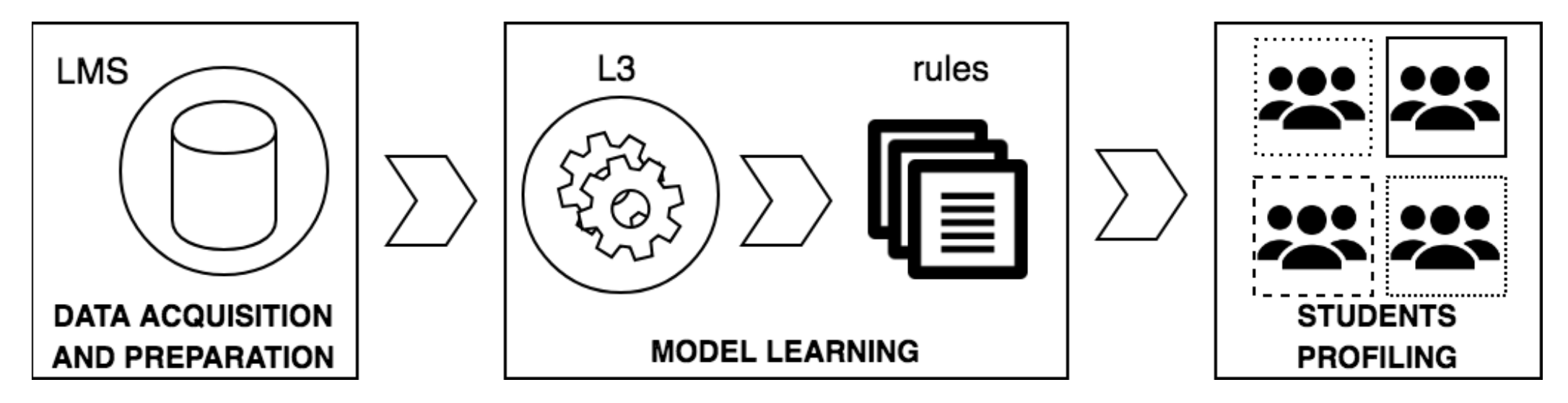
3. Materials and Methods

Associative classifiers are used to generate per-student predictions of the exam success rates. The architectural schema of the proposed methodology is depicted in Figure 1. The main steps can be summarized as follows.

• Data acquisition and preparation: Student-related data are acquired over the whole academic year by the Learning Management Systems (LMS) adopted by the university, collected into a unified repository, and prepared for the classification process.
• Associative model learning: Multiple associative classifiers, consisting of a selection of association rules [37], are trained from the prepared data at different time points (e.g., before student enrollment, before the beginning of the course, before the beginning of the examination session). Each classifier describes the most significant correlations between a combination of data features and the success rate of the upcoming exam.
• Model interpretation: The associative model is manually explored to identify at-risk/successful student profiles based on the extracted rules and to validate the per-student rate predictions based on the associated profile.

A more thorough description of each step is given in the following sections.

3.1. Data Acquisition and Preparation

Learning Management Systems are nowadays able to acquire, collect, and store data related to a variety of different student-related data. According to the classification given in [6], we may categorize the collected data features into the following categories:

• Student-specific characteristics, e.g., gender, age, ethnicity, high school type, standardized scores, current credit load.
• Student’s engagement indicators customized to the course under analysis, e.g., course satisfaction, frequency of logins to online portals, frequency of course materials’ accesses and downloads, frequency of video lectures’ accesses and downloads, number of discussions posted.
• Assessment scores: result of the entry test, grade earned in the previous exams.

In the proposed methodology the values of all the potentially relevant data features are acquired, collected in a unique repository (independently of their corresponding category), and stored into a relational dataset.

A relational dataset consists of a set of records, where each record is a set of items. In our context, items are pairs (feature, value). feature is a textual description of the student-related characteristics, while value is the corresponding value taken by the feature. More formal definitions of item and relational dataset follow.

Definition 1. Item.

Let $f_i$ be a label, called feature, which describes a peculiar student-related characteristics. Let ${\Omega }_i$ be the discrete domain of feature $f_i$. Each pair $(f_i,valu{e}_i)$, where $valu{e}_i\in {\Omega }_i$, is an item.

To deal with continuous attributes, the domain is discretized into intervals, where intervals are mapped into consecutive positive integers. For example, (Entry test result, From 70 to 85) is an item, which indicates that the grade earned by the student at the entry test is between 70 and 85.

Definition 2. Relational dataset.

Let $\mathcal{F}$ = $\{f_1,f_2,\dots ,f_n\}$ be a set of features and Ω = $\{{\Omega }_1,{\Omega }_2,\dots ,{\Omega }_n\}$ the corresponding domains. A relational dataset D is a set of records, where each record r is a set of items and contains at most one item for each feature in $\mathcal{F}$.

For classification purposes, a feature (hereafter denoted as class) is selected as prediction target. Hereafter, we will consider as class the success rate of the upcoming exam.

Definition 3. Labeled relational dataset.

Let D be a relational dataset and $\mathcal{F}$ = $\{f_1,f_2,\dots ,f_n\}$ its corresponding feature set. Let $f_n\in \mathcal{F}$ be the class and let ${\Omega }_n=C$ be the class domain. For each dataset record $r_i$ such that $r_i\in D$, let $c_i\in C$ be its class value. D is a labeled relational dataset.

A record r ∈ D for which the class value is known is called training (labeled) record. Conversely, a record $r_t\in D$ for which the value is unknown is called test (unlabeled) record.

Table 1. Running example.

Student	Entry Test	Accessed Video	Success Rate
Id	Grade	Lectures (%)	(Class)
101010	[60, 70]	<5	fail
202020	[80, 95]	[10, 20]	pass
303030	[60, 70]	<5	fail
404040	[70, 85]	[30, 40]	pass
505050	[60, 70]	[30, 40]	fail
606060	[70, 85]	[80, 90]	pass

reports an example of labeled training dataset whose records are related to different students of the Mathematical Analysis course at the same time point. Notice that the dataset contains both time-invariant features, e.g., the grade of the entry test (e.g., 65 over 100), and time-dependent ones, e.g., the number of accessed video-lectures). To predict the students’ success rates at a given time point, we can train the classifier on the running example dataset (excluding student ids) by setting as class the Success rate feature.

3.2. Associative Model Learning

Classification of relational data entails first generating a model from a set of (labeled) training records and then applying it to a set of (unlabeled) test records. Many different classification approaches have been proposed in literature (e.g., Bayesian classifiers, decision trees, Support Vector Machines (SVMs), Neural Networks, and associative classifiers). A relevant drawback of many classification techniques (e.g., Bayesian classifiers, SVMs, Neural Networks) is the limited explainability of the generated models. Predicting student academic performance by using non-explainable models entails fully trusting the prediction outcome, because the patterns used to assign the student’s success rate for a given course are unknown [38].

Decision trees and associative classifiers are the two main classes of explainable classification models. Users could explore these models in order to gain insights into classifiers’ decisions. Decision trees are popular classification techniques based on tree-based structures built on the training dataset [39]. Decision trees perform a greedy search for rules by heuristically selecting the most promising features. Such greedy (local) search may discard important rules. Associative classifiers, on the other hand, perform a global search for rules satisfying some quality constraints (i.e., minimum support) [40]. More specifically, as discussed in [41], decision trees suffer from the problem of adaptability since they could take decisions based on small samples of data and, therefore, the final classifier could not be representative of the overall trends. Associative classification overcomes the aforesaid problem by focusing on the features of the given test instance, thus increasing the chance of generating more rules that are useful for classifying the test instance. Association rules represent strong associations between sets of feature values and the class. Rules are extracted, filtered, and ordered prior to be included in the classification model. In this work we apply the rule extraction and selection methodologies adopted by the $L^3$ state-of-the-art algorithm [15]. A more detailed description of the rule extraction and evaluation steps is reported below.

Association rules. Let $\mathcal{D}$ be a relational dataset (see Definition 1) and let X be an arbitrary set of items in $\mathcal{D}$. An itemset is a set of items, i.e., a combination of feature values occurring in a dataset. In the context of relational data, X is an itemset if all of its items belong to distinct features.

Recalling the running example in Table 1, {(Fraction of video-lectures accessed, <5%), (Success rate, fail)} is an itemset representing the co-occurrence of two items (related to different features) in the source dataset. It indicates that the students who accessed less than 5% of the video-lectures of the course failed the exam.

Itemsets are characterized by their support value [37]. It indicates the fraction of records in the source dataset in which all the items in the itemset co-occur. For example, {(Entry test, [60, 70]), (Success rate, fail)} has support equal to 33% in the running example dataset, because the two items co-occur in two records out of six.

An association rule is an implication $X\to Y$, where X and Y are disjoint itemsets. A more formal definition follows.

Definition 4. Association rule.

Let X and Y be two itemsets in $\mathcal{D}$ such that $X\cap Y$=Ø. An association rule is represented in the form $R:X\to Y$, where X and Y are the body and the head of the rule respectively.

X and Y are also denoted as antecedent and consequent of rule $X\to Y$.

For example, {(Entry test, [60, 70]), (Video-lectures accessed, <5%)} → (Success rate, fail) is an association rule. It indicates that the co-occurrence of two specific conditions, i.e., passing the entry test with a grade between 60 and 70 and accessing less than 5% of the video-lectures, is correlated with an exam fail.

Association rule extraction is commonly driven by support (sup), confidence (conf), and correlation (corr) quality indexes [37]. The support of the rule indicates the frequency of occurrence of the implication in the source dataset, while the confidence index represents the rule strength.

Definition 5. Support of an association rule.

Let $\mathcal{D}$ be a relational dataset. The support (sup) of an association rule $R:X\to Y$ is defined as the support of $X\cup Y$ in $\mathcal{D}$.

Definition 6. Confidence of an association rule.

Let $\mathcal{D}$ be a relational dataset. The confidence (conf) of an association rule $R:X\to Y$ is the conditional probability of occurrence in $\mathcal{D}$ of itemset Y given itemset X, i.e., $conf\left(R\right)=\frac{sup(X\cup Y)}{sup\left(X\right)}$.

For example, the association rule {(Entry test, [60, 70]), (Video-lectures accessed, <5%)} → (Success rate, fail) has support equal to 33% and confidence equal to 100%, because in all the records in which the antecedent occurs the consequent occurs as well. In our context, the confidence index indicates that in all the cases in which the entry test grade is between 60 and 70 and the number of video-lectures accessed is very low the success rate is fail.

In some cases, measuring the strength of a rule in terms of support and confidence may be misleading [42]. When the rule consequent is characterized by relatively high support value, the corresponding rule may be characterized by a high confidence even if its actual strength is relatively low. To overcome this issue, the correlation (or lift) index [42] may be used to measure the (symmetric) correlation between body and head of the extracted rules.

Definition 7. Correlation of an association rule.

Let $X\to Y$ be an association rule. Its correlation index (corr) is given by $\mathrm{corr}(\mathrm{X},\mathrm{Y})=\frac{\mathrm{conf}(X\to Y)}{\sup \left(\mathrm{Y}\right)}=\frac{\sup (X\to Y)}{\sup \left(\mathrm{X}\right)\sup \left(\mathrm{Y}\right)}$, where $\sup (X\to Y)$ and $\mathrm{conf}(X\to Y)$ are, respectively, the rule support and confidence, and $\sup \left(X\right)$ and $\sup \left(Y\right)$ are the support counts of the rule antecedent and consequent.

If corr(X,Y) is equal to or close to 1, itemsets X and Y are not correlated with each other. Correlation values significantly below 1 show negative correlation, whereas values significantly above 1 indicate a positive correlation between itemsets X and Y, i.e., X and Y co-occur more than expected.

For example, the correlation of rule {(Entry test, [60, 70]), (Fraction of video-lectures accessed, <5%)} → {(Success rate, fail)} is $\frac{\frac{2}{6}}{\frac{2}{6}*\frac{3}{6}}=2$. Hence, the rule correlation is positive.

Classification rules. The $L^3$ classifier consists of a subset of high-quality association rules, hereafter denoted as strong classification rules. A classification rule [13] is an association rule whose consequent is a class item.

For example, rule {(Entry test, [60, 70]), (Fraction of video-lectures accessed, <5%)} → {(Success rate, fail)} is a classification rule.

Classification rules are selected because they can be directly applied to label test records whose non-class feature values match those appearing in the rule antecedent.

A classification rule is strong if its support, confidence, and correlation values are above (analyst-provided) thresholds.

High-Quality Rules

In [15], the strong classification rules are further partitioned into (i) high-quality rules, i.e., rules used in the classification of training data, and (ii) unchecked rules, that is, rules unused during the training phase, but potentially useful to classify test data. In the next step, we will exclusively consider high-quality rules.

3.3. Profile Extraction and Ranking

The associative models generated by the $L^3$ classifier at different time points are collected and analyzed to gain knowledge about classifiers’ decisions.

Classification rules related to rate fail describe at-risk student profiles. For example, rule {(Entry test, [60, 70]), (Fraction of video-lectures accessed, <5%)} → {(Success rate, fail)} describes a profile of students who have achieved fairly good test outcomes and who have not downloaded the video-recordings of the in-class lectures. Conversely, classification rules related to rate pass describe successful student profiles.

Profiles can be classified as (i) at-risk profiles, if they are peculiar to the success rate fail, or (ii) successful profiles, if they are peculiar to success rate pass. Note that profiles are peculiar to a given course and period of time. Hence, they may change while considering different courses and periods. Further profile categorizations can be based on the number and type of features involved. Specifically,

• Single-feature profiles are profiles characterized by a single feature category. According to the feature categorization reported in Section 3.1, they can be further classified as profiles on student-specific characteristics (SSC profiles, in short), profiles on student’s engagement indicators (SEI profiles), or profiles on assessment scores (AS profiles) depending on the category of the reference feature.
• Mixed-feature profiles are profiles that are modeled on multiple data feature categories. They extend single-feature profiles by combining features of different categories.

While single-feature profiles could be identified also using decision tree models, mixed-feature ones are peculiar to associative models, which encompass rules including items belonging to multiple features in the rule antecedent. For the sake of simplicity, mixed-feature profile categories will be denoted by combining the same abbreviations indicated above of single-feature profiles. For example, SSC+AS profiles are those characterized by features belonging to both student-specific characteristics and assessment scores.

For example, rule {(Entry test, [60, 70]), (Fraction of video-lectures accessed, <5%)} → {(Success rate, fail)} can be considered to build an at-risk SEI+AS profile, because the assigned success rate is fail, while the non-class features in the rule antecedent belong to classes Student’s engagement indicators and Assessment scores, respectively.

Teachers could be interested either in looking at the profile associated with a specific student or in identifying the most recurrent student profiles. In the latter case, once an associative model has already been applied to a significant number of students, the corresponding profiles can be filtered based on their actual usage. Specifically, identifying which classification rules have actually been applied by the classifier to each student allows teachers to associate students with recurrent risk profiles. For example, if rule {(Entry test, [60, 70]), (Fraction of video-lectures accessed, <5%)} → {(Success rate, fail)} has been used to classify 5% of students, then the corresponding at-risk profile could be deemed as particularly relevant to understand the career progress of the students.

At-risk and successful profiles are first ranked by decreasing number of classified students. Then, the top ranked profiles are manually explored in order to gain insight into the analyzed students. When the students described by a profile have attended the course exam, exam outcomes are used to discriminate between reliable profiles and not. For example, if the majority of the students who were classified using rule {(Entry test, [60, 70]), (Fraction of video-lectures accessed, <5%)} → {(Success rate, fail)} actually failed the exam, then the corresponding profile could be deemed as reliable.

Analyzing reliable students profiles well before the end of the course allows teachers to perform timely interventions. For each profile, one or more targeted actions can be recommended. Actions targeted to reliable at-risk profiles are preventive, because their aim is to prevent failures. Conversely, actions targeted to reliable successful profiles are aimed at reinforcing good practices.

For example, let us suppose that, based on the exploration of the mined rules, a mixed-feature at-risk profile, consisting of all students whose entry test grade is below average and whose percentage of accessed video lectures is very low (<5%), is identified. A strong correlation between entry test grades and accessed video lectures and exams’ outcome could prompt university managers to plan (i) additional courses on basic concepts tailored to at-risk students or (ii) reinforcement actions triggered by the discovered profile (e.g., send reminders throughout the course notifying the publication of new materials) Similarly, a profile may represent foreign students who have neither downloaded nor accessed using streaming the video lectures of the course. Periodic recommendations targeted to inactive students can be exploited to foster students’ engagement.

4. Results

We empirically analyzed the applicability of the proposed methodology on student-related data acquired by our technical university.

To perform quantitative and qualitative evaluation on the analyzed data, we run experiments on an Intel(R) Core(TM) i7-8550U CPU with 16 GB of RAM running Ubuntu 18.04 server.

4.1. Learning Context and Related Data

The university provides B.S. and M.S. engineering courses and adopts a blended learning model. The blended model relies on a massive educational video service, which delivers video recordings of the in-class lectures. The access to the video lectures of a course is allowed to all the enrolled students. Hence, students can exploit video lectures as complementary materials in addition to in-class lectures [43]. Since 2010 the university has video-recorded in the classroom all the courses of the first year of the B.S. in Engineering, that is common to all B.S. engineering curricula. The number of students enrolled to the 1st-year courses is approximately 5000 per academic year.

The learning platform of the university traces the students’ interactions with the provided educational materials. Specifically, through the platform students can (i) access and download educational materials (e.g., slides, lecture notes, exam simulations), and (ii) watch (streamed from the educational Web service or downloaded) the video-records of the in-class lectures.

As a case study, we applied the proposed methodology on data acquired in the academic year 2018–2019. Specifically, we focused on predicting the exam success rate for all the students enrolled to the 1st-year B.S. courses. The 1st-year curricula encompasses the following courses: Mathematical Analysis (MA), Chemistry (CH), Computer Science (CS), Linear Algebra (LA), and Physics (PH), plus an elective course which is not considered in the present analysis because data are not comparable. In the considered academic year, courses MA, CH, and CS were held in the first semester (i.e., from 1 October 2018 to 15 January 2019), while courses LA and PH were held in the second semester (from 1 March 2019 to 15 June 2019).

Three examination sessions were scheduled within an academic year: (i) the 1st semester (winter) session, which is held at the end of the first semester (i.e., from 22 January 2019 to 28 February 2019), (ii) the 2nd semester (summer) session, which is held at the end of the second semester (i.e., from 16 June 2019 to 22 July 2019), (iii) the autumn session, which is held after the summer break (i.e., from 1 September 2019 to 30 September 2019). Students are free to attend any and all examination sessions, provided that they have already attended the course.

To early identify at-risk students, for each student and exam we predicted the success rate in the upcoming examination session. Specifically, we trained separate classifiers at the twelve different time points reported in

Table 2. Time points of prediction.

Id	Time Point	Description
$t_0$	31 August 2018	Before entry test
$t_1$	7 September 2018	After entry test
$t_2$	30 October 2018	Early 1st semester
$t_3$	31 November 2018	Mid-way 1st semester
$t_4$	15 January 2019	Close to 1st semester exams
$t_5$	22 January 2019	Start of 1st semester exam session
$t_6$	28 February 2019	End of 1st semester exam session
$t_7$	31 March 2019	Early 2nd semester
$t_8$	30 April 019	Mid-way 2nd semester
$t_9$	15 June 2019	Start of 2nd semester exam session
$t_{10}$	22 July 2019	End of 2nd semester exam session
$t_{11}$	31 August 2019	After summer break

. For the sake of brevity, each time point will be hereafter denoted by the corresponding identifier. At each time point we predicted the outcome of the considered student in the upcoming exam (independently of the actual exam attendance). More specifically, for the 1st-semester courses (MA, CH, CS) at time points from $t_0$ to $t_5$ we predicted the success rate of the winter session exam, from points $t_6$ to $t_9$ we predicted the success rate of the exam held in the summer session, while at points $t_{10}$ and $t_{11}$ we predicted the rate of the autumn session. For the 2nd semester courses, from $t_0$ to $t_9$ we predicted the success rate of the exam in the summer session (because the winter session is not eligible for students at first enrolment), while at points $t_{10}$ and $t_{11}$ we predicted the rate of the autumn session.

For the courses held in the first semester (MA, CH, and CS), the first exam after course attendance is scheduled in the winter session, while for the other courses (LA, PH) the first exam is scheduled in the summer session. However, for all the 1st-year courses students may undergo the corresponding exam in any of the aforesaid sessions (e.g., they can undergo the MA exam the first time during the summer session).

Details on the Source Data

The considered data source consists of two main tables: table Students collects general information about the students, whereas table Courses-Activities collects information about course attendance. The schema of each table is detailed in

Table 3. Schema of the Students table.

Attribute	Description	Data Type	Domain
Student Id	student identifier	categorical	{1,2......}
Gender	gender	categorical	{M = male, F = female}
Age	student’s age—average students’ age	ordinal	{−1,1,2,3}
BH-loc	country of birth identifier	categorical	{AF, AL,...}
HM-loc	home country identifier	categorical	{AF, AL,...}
HS-loc	high school country identifier	categorical	{AF, AL,...,}
HS-gr	high school grade band	ordinal	{1 = low, 2 = low average, 3 = average, 4 = average high, 5 = high}
GRE-gr	entry test grade	ordinal	{1 = low, 2 = low average, 3 = average, 4 = average high, 5 = high}
BS course	bachelor’s degree track	categorical	{mechanical engineering, computer enginnering...}

and

Table 4. Schema of the Courses-Activities table.

Attribute	Description	Data Type	Domain
Student Id	student identifier	categorical	{1,2......}
Course Id	course identifier	categorical	{1,2......}
Time point	time point identifier	ordinal	{0,1,...,12}
MA-mat	discretized frequency of video lectures’ downloads normalized to the maximum number of downloads made up to that point in time	categorical	{H = high, F = average, L = little, N = no use}
MA-str	discretized frequency of video lectures’ accesses normalized to the maximum number of accesses up to that point in time	categorical	{H = high, F = average, L = little, N = no use}

. The analyzed tables do not contain any missing value. We generated a training dataset from the original tables, where each dataset record corresponds to a distinct pair of Time Id and Course Id values.

Table 5. Data samples per time point.

	${\mathit{t}}_0-{\mathit{t}}_5$		${\mathit{t}}_6-{\mathit{t}}_9$		${\mathit{t}}_{10}-{\mathit{t}}_{11}$
	Pass	Fail	Pass	Fail	Pass	Fail
MA	1515	2577	1183	332	1035	148
CS	1786	2307	1427	359	1127	300
CH	2697	1394	2397	300	2135	262
PH	2823	1270	2823	1270	2431	392
LA	1245	2848	1245	2848	1018	227

reports the number of records per time point and course as well as the percentage of records per class. It indicates for each course the number of students considered in the training data at different time points. For example, for the MA course at time points from $t_0$ to $t_5$ (i.e., before the first examination) training data consist of 4092 students, among which 1515 students who will pass the upcoming exam and 2577 students who will fail it.

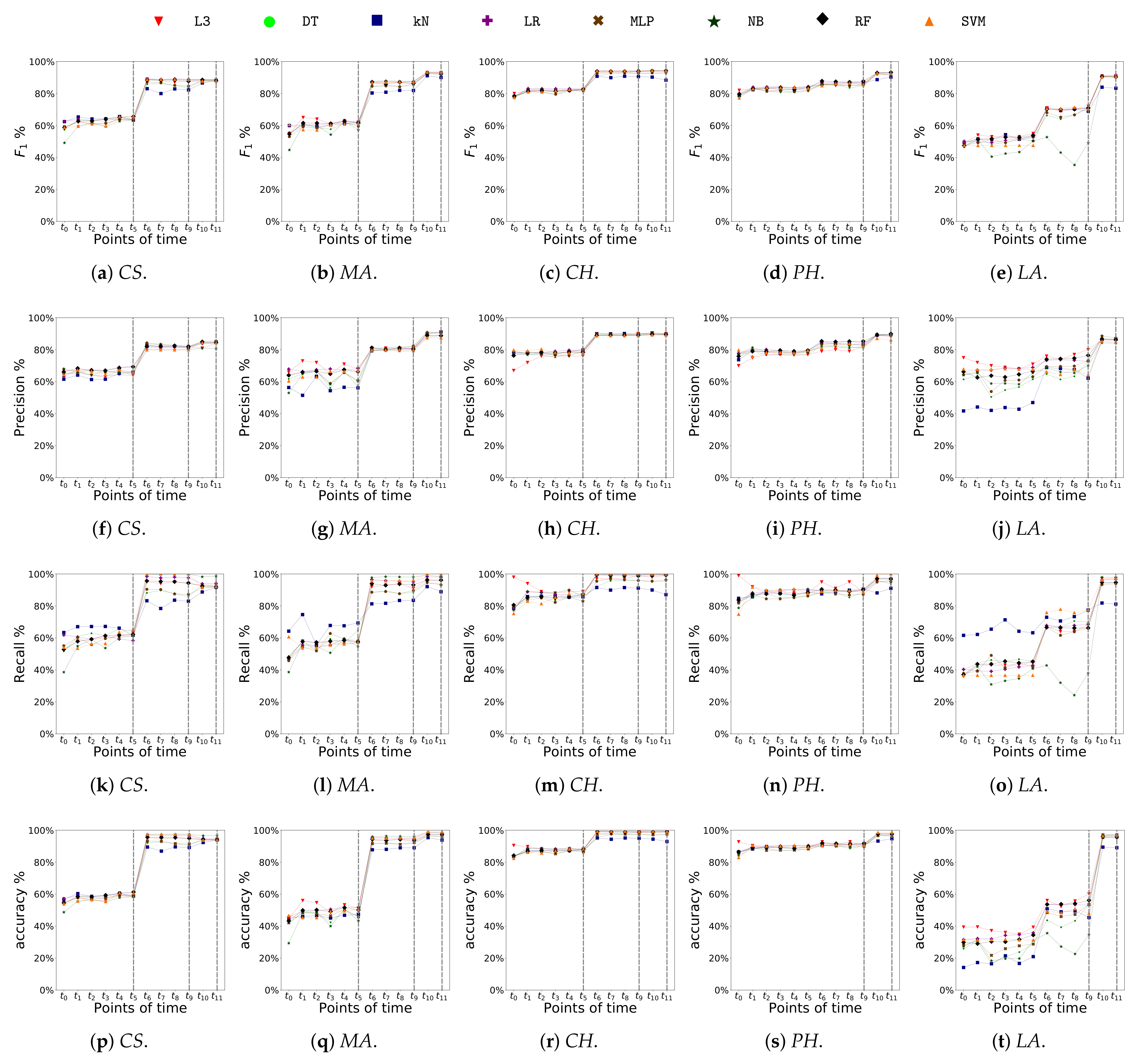
4.2. Performance Comparison between Different Algorithms

We conducted an empirical evaluation of the performance of various classification algorithms on the analyzed dataset. The goal of the experimental analysis is to answer to the following research question (RQ1): Are associative classifiers as accurate as the best performing ones in predicting student academic performance?

To address the above issue, we compared the performance of the $L^3$ classifier with that of a variety of other classifiers. Notice that despite similar experimental comparisons have already been conducted in previous studies (e.g., [3]), to the best of our knowledge associative models have not been considered yet.

Classification models

We considered the following classifiers [39]:

• The Live and Let Live ($L^3$) classifier [15]: a state-of-the-art associative classifier.
• C4.5 (DT): popular decision tree-based classifiers.
• Multi-Layer Perceptron (MLP): a popular single-layer Neural Networks model.
• LIBSVM (SVM): an established Support Vector Machines model.
• Multinomial naive Bayes (NB): an established multiclass Bayesian classifier.
• k-Nearest Neighbor (kNN): a lazy distance-based classifier (lazy classifiers do not create models, but on-the-fly compute the distances between a test record and each of the training records).
• Random Forest (RF): ensemble method.

For the $L^3$ classifier we used the C++ implementation provided by the authors, while for all the other algorithms we used the Python implementations available in the Scikit-Learn library [44]. To tune classifier performance at each considered time point, we performed a grid search by varying the values of the most significant parameters. Hereafter, for the sake of brevity, we will report the results achieved by the best configuration separately for each algorithm.

Time complexity

The time complexity for training and testing the classification models ranged between few seconds on simpler datasets (e.g., 7 s for MLP, 31 s for $L^3$) to approximately one hour in the worst cases. However, most prediction models were generated in less than 60 s.

Performance metrics

To quantitatively evaluate classifier performance at each time point, we applied a stratified 5-fold cross-validation strategy and computed the following performance metrics:

• Precision of class fail: It is the ratio between number of students who have been correctly labeled as belonging to class fail ($TN$) divided by the total number of students assigned to class fail ($TN+FN$).
• Recall of class fail: It is the ratio between number of students who have been correctly labeled as belonging to class fail ($TN$) divided by the total number of students who actually belong to class fail ($TN+FP$).
• F1-score of class fail: It is the harmonic mean of precision and recall of class fail.
• Balanced Accuracy: It is the average of the recall computed over the two classes and is given by $\frac{1}{2}(\frac{TP}{TP+FP}+\frac{TN}{TN+FN})$ [45]. It evaluates the ability of the classifier to correctly assign both class labels. It is especially useful when the classes are imbalanced in the test sample since it rewards the correct predictions on the minority class. When the test samples are balanced over the two classes, it corresponds to the conventional accuracy measure (i.e., percentage of correct predictions).

While the accuracy measure is independent of the class, the other metrics are specific to class fail. Since the main goal of student performance prediction is to early detect at-risk students, we specifically analyzed the ability of the classifiers to correctly classify this particular category of students.

Figure 2a–f plot for each course the accuracy scores achieved by the classifiers at different time points. The vertical dashed lines indicate the examination sessions scheduled during the academic year. The accuracy values achieved by most of the algorithms before the beginning of the first semester is around 60%. For the 1st semester courses (MA, CH, CS) the performance decreases after the first examination session, because predicting students’ outcomes at the next sessions (i.e., at the second trial) is significantly more challenging. For the 2nd semester courses (PH, LA) similar results were achieved after the first examination, which is scheduled after time $t_9$. $L^3$ performed as good as the best performing classifiers (K-NN, MLP) while decision tree classifiers (DT and RF) performed worse. Slight fluctuations in the series of accuracy values have shown in the last time points ($t_9$–$t_{11}$). The reason is that since the number of students under evaluation decreases (because the majority of them have already passed the exams), the models are less robust and more sensitive to noise.

Figure 2f–t, respectively, plot for each course the F1-score, precision, and recall of class fail achieved by the classifiers at different time points. They describe the ability of the classifiers to accurately predict exam failures. Precision and recall values increase as time goes by (e.g., for MA the $L^3$ precision ranges from 65% at $t_0$ to 90% $t_{10}$). The recall values significantly increase after the first examination session (at $t_5$ for the 1st semester courses, at $t_9$ for the 2st semester ones) because students who failed once are more likely to fail again. $L^3$ performed as good as the best performing classifiers for all the courses and for most of the considered time points.

In order to assess the statistical significance of the performance variations (computed in terms of accuracy, F1-score, precision, and recall of the class fail), we applied the Wilcoxon signed rank t-tests [46] using a significance level equal to 0.5%. The results show that $L^3$ performed significantly better than DT and RF at specific time points for the majority of the analyzed courses, while it performed as good as the best performing approaches (K-NN, MLP). Hence, the $L^3$ associative model could be deemed as a reliable model for early predicting student performance.

4.3. Model Exploration

To explore the high-quality rules generated by the $L^3$ classifier we focused the attention on the most reliable student profiles. Specifically, we first counted, for each high-quality rule, the number of classified students as well as the percentages of correctly and incorrectly classified ones. Next, we analyzed the subset of high-quality rules that (i) have been applied to at least 1% of the students, and (ii) have exclusively produced correct predictions. All the other rules were discarded, as they potentially generated unreliable predictions. Rule exploration aims at answering the research questions RQ2 and RQ3 posed in Section 1. It entails exploring model interpretability since the extracted rules can be easily understood by non-expert end-users.

Research question (RQ2): What are the most discriminating features to forecast the exam success rates at different time points?

To answer to this question, we analyzed the frequency of occurrence of the single features and of the pairs of features in the selected student profiles.

Figure 3 shows the percentage of rules including specific features in their antecedent at three representative time points: $t_0$ (before the entry test), $t_1$ (after the entry test and the BS course choice, but before the start of the semester) and $t_5$ (at the end of the first semester). The plot highlights the features that mostly influence student performance separately for each course and time point. At $t_0$ only the student-specific features are considered and, unsurprisingly, the most important one is the high school grade (HS-gr). Age turned to be strongly correlated with the success rate as well, because students who are older than average often achieved bad results during high school. At $t_1$ the entry test grade (GRE-gr) plays a significant role in rate prediction, in combination with HS-gr. The BS course choice (e.g., mechanical engineering vs computer science engineering) is also an important feature, because the attitude of the students towards the different disciplines depends on the perceived importance in their future. At $t_5$ the effect of the download of educational material (e.g., MA-mat) and of the streaming activity (e.g., MA-str) for the different courses are visible. The high school degree remains very relevant, while in general age decreases its importance. The activities carried out in one course may influence other courses. For example, since MA provides students with the basic concepts for both LA and PH, the exam grade (whenever available) is particularly discriminating.

The radar plots in Figure 4 deepen the feature analysis for the 2nd-semester LA course. Features are grouped in different categories (personal data and scholastic history, entry test and BS course choice, activity in two sample courses, MA and CS, educational material download and exam success) and their importance is compared at all the time points (from 0 to 9). For example, graph (a) confirms that the high school grade (HS-gr) has an important impact on student performance during the whole academic year. On the contrary, gender is relevant only at the beginning, because the student activity during the semester becomes more and more important to foresee exam success rate. Graph (b) shows that the test grade (GRE-gr) and the BS course choice have an impact only in the first semester, and during the second semester (when the LA course is on) other features become much more important. Graph (c), about students’ activity in the MA course, shows that studying MA is strongly related to passing the LA exam. It also evidences that the streaming activity (MA-str) is mainly relevant at the end of the semester and during the exam break: students use educational materials from the beginning of the semester, but concentrate the streaming activity closer to exam sessions. Graph (e) shows that passing the 1st-semester exams (MA-gr, CH-gr, CS-gr) has a strong influence on passing LA in the second semester (the influence is higher in case of MA than CS, coherently with the topic focus). The performance in the first semester of the first year is probably the most discriminating factor in classifying students as active or inactive.

Extracting association rules allows us to explore the most relevant item co-occurrences relative to different feature combinations [40]. Figure 5 shows the importance of a subset of relevant combinations of feature for LA at different time points. For example, the scholar history (HS-loc, HS-gr) is relevant to predict success rate before any university activity (i.e., before $t_1$), including entry test and BS course choice. After that, and until almost the end of the semester ($t_4$), the high school grade and the entry test grade coupled with the BS course choice (HS-gr, BS course), (GRE-gr, BS course) became the most relevant feature combination. During the first semester (from $t_2$ to $t_5$) educational material download of two courses has the strongest effect (MA-mat, CS-mat), showing student active participation. Finally, during the second semester (when LA is given), the most relevant feature combination is the number of downloads of educational material combined with the grade achieved for the MA course (LA-mat, MA-gr).

Research question (RQ3): which combinations of feature values have been frequently used to assign the exam success rates?

Table 6. High-quality single-feature rules mined from the MA datasets including only SSC features. minsup = 1%, minconf = 50%, mincorr = 2. Support and confidence values of each of the selected rules are averaged over the 5 cross-validation folds (average and standard deviation are specified).

Num	Time ID	Body	Head	Support (%)	Confidence (%)	Lift	Description
Pre-test
1	$t_0$	HS-loc = Italy, HS-gr = 5, gender = F	pass	10.0 ± 0.3	86.5 ± 0.7	7	Very good high school grade, high school in Italy, female (independently of age)
2	$t_0$	HS-loc = Italy, HS-gr = 4, age = 0	pass	30.4 ± 0.2	79.2 ± 1.3	8	Good high school grade, high school in Italy, average age
3	$t_0$	HS-gr = 5, gender = M, age = −1	pass	14.1 ± 0.2	87.9 ± 1.0	4	Good high school grade, male, younger than average (independently of the high school country)
4	$t_0$	HS-gr = 1, gender = M, age = 3	fail	3.0 ± 0.1	90.7 ± 1.2	3	Very low high school grade, male, much older than average
5	$t_0$	HS-gr = 2, age = 1	fail	3.9 ± 0.1	89.7 ± 1.3	8	Low grade, older than average (independently of gender and high school country)

,

Table 7. High-quality single-feature rules mined from the MA datasets including only T-MAT features. minsup = 1%, minconf = 50%, mincorr = 2. Support and confidence values of each of the selected rules are averaged over the 5 cross-validation folds (average and standard deviation are specified).

Num	Time ID	Body	Head	Support (%)	Confidence (%)	Lift	Description	Similar Rules
Early 1st semester
6	$t_2$	MA-mat = L	pass	31.8 ± 0.2	68 ± 0.6	7	Little use of MA material, but already at the beginning of the semester	CH (with fail)
7	$t_2$	MA-mat = F	pass	14.9 ± 0.3	75.2 ± 0.7	8	Average use of MA material	CH
8	$t_2$	CS-mat = L, CH-mat = L	pass	14.9 ± 0.1	68.3 ± 0.7	9	Little use of other courses material	CS
9	$t_2$	MA-mat = N, CS-mat = N, CH-mat = N	fail	65.4 ± 0.1	65.5 ± 0.7	6	No use of material (inactive)	CH, CS
Mid-way 1st semester
10	$t_3$	MA-mat = H	pass	7.5 ± 0.3	78.9 ± 1.3	7	High use of MA material	CH
11	$t_3$	MA-mat = F	pass	21.1 ± 0.2	76.1 ± 0.8	7	Average use of MA materials, confirms $t_2$
12	$t_3$	MA-mat = L	fail	25.2 ± 0.2	64.4 ± 0.5	7	Little use of MA material is not enough now (cfr $t_2$)	CH, CS
13	$t_3$	MA-mat = N, CS-mat = N, CH-mat = N	fail	17.2 ± 0.2	87.4 ± 1.3	8	No use of material (inactive), confirms $t_2$	CH, CS
Close to 1st semester exams
14	$t_4$	MA-mat = F	pass	25.9 ± 0.1	78.2 ± 1.1	7	Average use of MA material, confirms $t_2$ and $t_3$	CH, CS
15	$t_4$	MA-mat = L	fail	25.2 ± 0.1	73.9 ± 0.8	8	Little use of MA material, confirms $t_3$	CH, CS
16	$t_4$	MA-mat = N, CS-mat = N, CH-mat = N	fail	13.2 ± 0.1	95.7 ± 0.6	7	No use of material (inactive), confirms $t_2$ and $t_3$	CH, CS
17	$t_4$	CH-mat = H	fail	3.9 ± 0.1	78.8 ± 0.8	8	High use of another course material	CS (with pass)

,

Table 8. High-quality rules mined from the MA datasets including only STREAM-VL features. minsup = 1%, minconf = 50%, mincorr = 2. Support and confidence values of each of the selected rules are averaged over the 5 cross-validation folds (average and standard deviation are specified).

Num	Time ID	Body	Head	Support (%)	Confidence (%)	Lift	Description	Similar Rules
Early 1st semester
18	$t_2$	MA-str=L	pass	24.2 ± 0.2	70.0 ± 0.7	6	Little use of MA videos, but soon (october), coherent with MA material	CH (with fail), CS (with fail)
19	$t_2$	CH-str = L	pass	20.1 ± 0.2	71.7 ± 1.2	4	Streaming of other courses has positive impact even if no MA videos (shows students’ engagement)	CS, CH (with fail)
		CS-str = L		12.4 ± 0.1	69.1 ± 0.7	6
		MA-str = N, CH-str = L		7.6 ± 0.3	72.5 ± 0.3	5
		MA-str = N, CS-str = L		5.5 ± 0.2	70.9 ± 0.9	8
Mid-way 1st semester
20	$t_3$	MA-str = L	pass	29.1	69	6	Little of MA videos is enough, with or without other courses. Different from MA material: just-enough approach for video streaming	not CS (fail)
		MA-str = L, CH-str = L		15.2 ± 0.1	70.6 ± 0.9	7
		MA-str = L, CS-str = L, CH-str = N		10.4 ± 0.1	70.2 ± 0.2	7
21	$t_3$	CH-str = L	pass	24.9 ± 0.3	70.6 ± 1.3	4	Streaming of other courses has positive impact, confirms $t_2$	CS, CH (with fail)
		CS-str = L, MA-str = N, CH-str = N		18.4 ± 0.2	68.2 ± 0.7	6
Close to 1st semester exams
22	$t_4$	MA-str = L, CH-str = L	pass	18.6 ± 0.2	69.9 ± 0.7	7	Little of MA videos is enough, confirms $t_3$	CS (with fail)
23	$t_4$	MA-str = F, CH-str = F	pass	28.9 ± 0.2	70.2 ± 0.7	4	Streaming of other courses has positive impact, confirms $t_2$ and $t_3$	CS, CH (with fail)
		MA-str = F, CS-str = F		10.7 ± 0.2	69.6 ± 0.9	7

and

Table 9. High-quality mixed-feature rules mined from the MA datasets. minsup = 1%, minconf = 50%, mincorr = 2. Support and confidence values of each of the selected rules are averaged over the 5 cross-validation folds (average and standard deviation are specified).

Num	Time ID	Body	Head	Support (%)	Confidence (%)	Lift	Description
Early 1st semester
24	$t_2$	MA-mat = N, MA-str = L	pass	7.5 ± 0.1	90.2 ± 0.9	45	Streaming is effective even without access to material
25	$t_2$	MA-mat = N, MA-down = L	fail	4.0 ± 0.1	65.2 ± 1.2	41	Download is not effective without access to material
Mid-way 1st semester—same rules
Close to 1st semester exams—same rules

report a selection of high-quality rules of different types extracted from the datasets of a representative course (MA). Specifically, Table 6, Table 7 and Table 8, respectively, report the selected single-feature rules extracted from each feature set (SSC, T-MAT, STREAM-VL), while Table 9 reports a selection of mixed-feature rules. For each rule we report the average support and confidence values computed over all the five cross-validation folds as well as their corresponding standard deviations.

The table content is organized as follows. Each rule has a progressive number. For each rule we report the time point at which the rule was extracted (from $t_0$ to $t_{11}$, according to the notation introduced in Table 2) and its content (in the form body → head) as well as its main quality indices. For the sake of brevity, the discretized feature values within each rule are abbreviated as None (N), Low (L), Fair (F), or High (H). Since similar rules may be extracted for the other courses, for each rule we indicated which courses have similar rules in column Similar rules. Finally, a short comment on the rule is given in Column Description.

The rules give interesting insights into the career progress of the enrolled students. For example, rule 4 in Table 6 indicates that the students who received fairly low admission grades and who are older than average are more likely to fail the MA exam. To prevent exam failures, the university could organize recovery courses for the students who have not achieved a sufficient grade in the part of the admission tests related to mathematics.

Rule 10 in Table 7 indicates that the students who have downloaded a large part of the educational materials by the first half of the MA course are likely to pass the exam. The extraction of such a profile prompts specific reinforcement action, i.e., stressing the importance of using educational material and encourage students to keep going like they are doing.

Rule 25 in Table 9 indicates that the students who have just downloaded the video-recording of the MA course without accessing the rest of the teaching materials are less likely to pass the exam in the upcoming session, because the number of downloads is positively correlated with the success rate only in conjunction with other indicators (e.g., a high number of accesses to the teaching materials). Conversely, the number of streaming accesses to the video-lectures is correlated with the success rate independently of the other features (see rule 24).

4.4. Takeaways

In light of the outcomes of the feature analysis and of the rule exploration in Section 4.3, the following conclusions can be drawn:

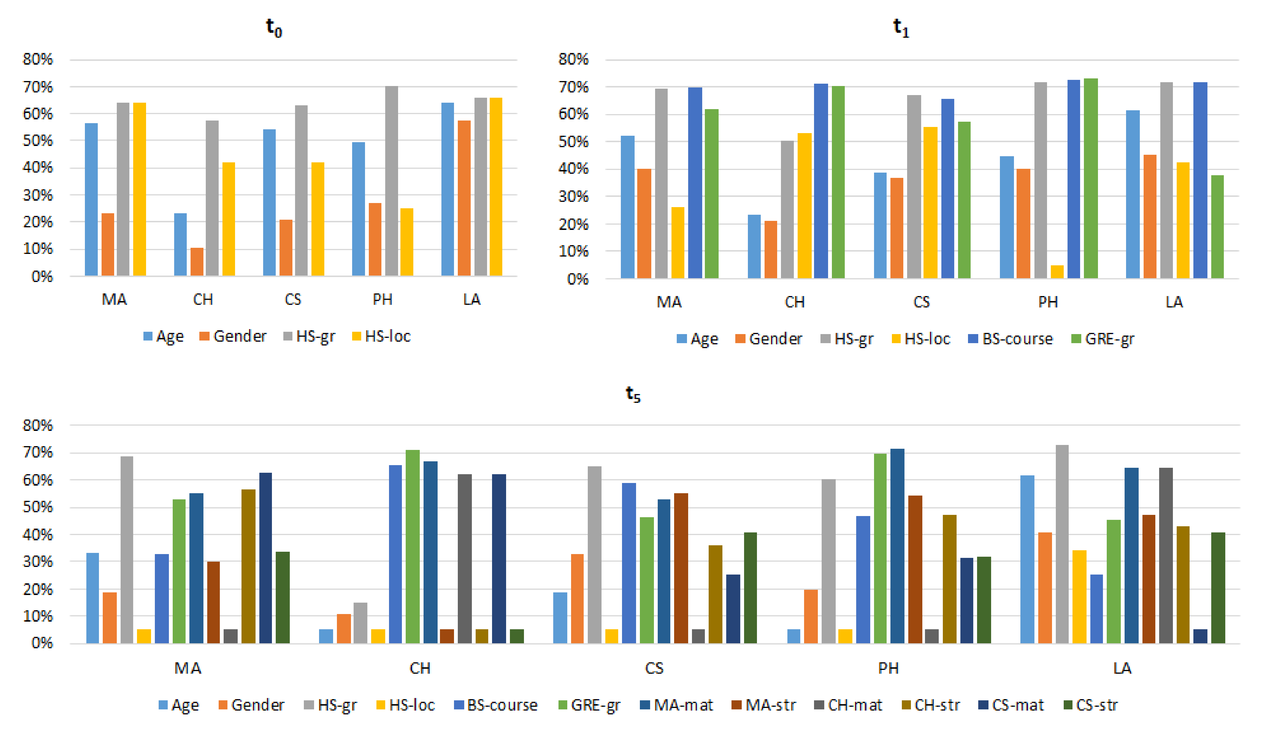
• The high school degree heavily influence students’ performance. In the example rules, this is already evident at $t_0$ (see Table 6) for the MA course, but the feature is very relevant during the whole academic year (see (a) in Figure 4) and the result is valid for all the courses (see Figure 3). Planning ad hoc remedial courses for students with low high school grade is therefore a suitable action to prevent student drop-out.
• Age has also a significant impact. This is not surprising because students that are older than the average likely had below average results during high school or are part-time workers. Rules 3, 4 and 5 in Table 6 confirm this statement for the MA course, but the feature is always relevant, especially in the first part of the academic year (see (a) in Figure 4) and the result is valid for the majority of the courses (see Figure 3). The fact that the influence of this feature decreases during the semester shows that motivated students learn to react putting extra effort in the study. Awareness actions toward this category of student can have a positive effect.
• Inactivity as regards educational material download is strongly related to failure. Rules 9, 13, and 16 reported in Table 7 for the MA course show that this holds during the whole semester. A proactive, reiterated invitation to use available educational materials could help students.
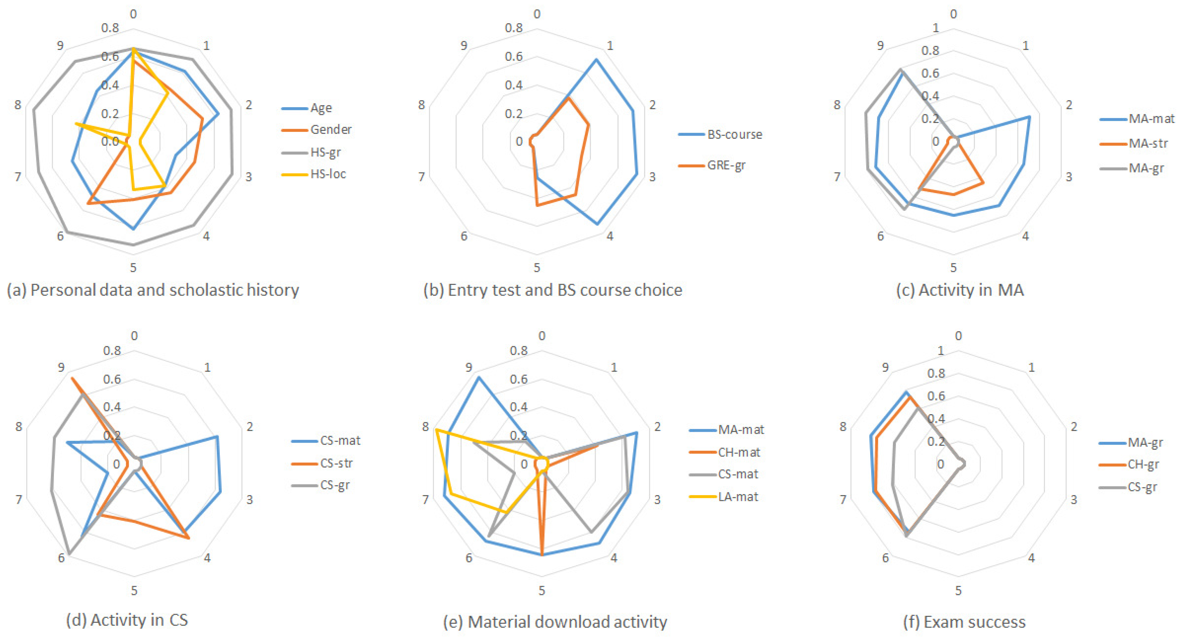
• It is very important to start the study activity very soon.Table 7 shows that a limited number of downloads of the MA educational materials is enough at the beginning of the semester (rule 6), but it is not later on (rules 12 and 15). This result is coherent with graph (e) in Figure 4: the educational material download activity has a strong influence on student performance already at the beginning of the semester. This is a useful recommendation for the students who want to improve their academic performance.
• Putting effort on many courses at the same time is a strategy that pays at the beginning of the semester but not close to the exam session. Rules 8 in Table 7 show that working on more that one course at $t_2$ increases the chance to pass the MA course, while rule 17 shows that the same kind of behaviour at $t_4$ yields opposite effects. Students should therefore be invited to work hard since the beginning of the semester, but they should also be warned that they should focus on a specific course when they are close to the exam.
• The use of the video-lecture streaming service is always positive.Table 8 shows that video-lecture streaming activity, even if limited, has a positive impact on passing the MA exam. This is valid for the use of MA video-lectures (rules 18, 20 and 22), but also for the use other course video-lectures (rules 19, 21 and 23), because this activity likely identifies active and motivated students. Rule 24 in Table 9 adds that streaming is positive even without downloading educational material. This outcome is very positive for our institution, since it proves that the video-lecture service is valuable, besides being appreciated by the students. Encouraging students to actively use the service is another fruitful action to prevent failure and drop-out.
• Downloading video-lectures is not enough. Rule 25 in Table 9 shows that video-lectures download without use of educational material is not enough to pass the MA exam. This rule identifies the students that simply download all the video-lectures for a later use, but that very likely (since they do not download the accompanying educational material) do not actually watch them. This result is supported by what is evident in graphs (c) and (d) of Figure 4. Video-lecture streaming activity and educational material download activity are shown to be indicators for exam success, while this is not the case for the video-lectures download activity.

5. Conclusions

The paper proposes to exploit associative classification to early predict student academic performance. Associative models are shown to be as accurate as the best performing classifiers on real student-related data acquired by our university. Thanks to the interpretability of associative models, domain experts can identify relevant at-risk and successful student profiles. Thanks to their explainability, they can also validate the assignments of the exam success rates by exploring the rules applied during the classification phase.

In the reported case study, the analysis of the rule-based models has allowed us to classify as at-risk students the ones with any combination of the characteristics enumerated below: (i) low high-school or entry test grades; (ii) older than the average; (iii) limited use of educational material, in general, or simply download video-lectures (no streaming); (iv) do not start to work from the beginning of the semester; (v) do not concentrate their effort on one course at a time close to the exam session. The achieved results confirm the applicability of the proposed methodology and open the following research questions, which we plan to address as future work.

• Is the associative model effective in predictive exams’ outcomes in other learning contexts (e.g., higher level courses, university-level M.S. courses)?
• Could associative models be integrated into an automated decision support systems that triggers personalized alerts based on the outcomes of the early prediction process?
• How can student profiles be effectively processed and visualized in order to continuously monitor the advances in the students’ learning process?

References

1. Siemens, G.; Baker, R.S.J.d. Learning Analytics and Educational Data Mining: Towards Communication and Collaboration. In Proceedings of the 2nd International Conference on Learning Analytics and Knowledge; ACM: New York, NY, USA, 2012; LAK ’12; pp. 252–254. [Google Scholar] [CrossRef]
2. Romero, C.; Ventura, S. Guest Editorial: Special Issue on Early Prediction and Supporting of Learning Performance. IEEE Trans. Learn. Technol. 2019, 12, 145–147. [Google Scholar] [CrossRef]
3. Conijn, R.; Snijders, C.; Kleingeld, A.; Matzat, U. Predicting Student Performance from LMS Data: A Comparison of 17 Blended Courses Using Moodle LMS. IEEE Trans. Learn. Technol. 2017, 10, 17–29. [Google Scholar] [CrossRef]
4. Adejo, O.W.; Connolly, T. Predicting student academic performance using multi-model heterogeneous ensemble approach. J. Appl. Res. High. Educ. 2018, 10, 61–75. [Google Scholar] [CrossRef]
5. Yang, T.Y.; Brinton, C.G.; Joe-Wong, C.; Chiang, M. Behavior-Based Grade Prediction for MOOCs Via Time Series Neural Networks. IEEE J. Sel. Top. Signal Process. 2017, 11, 716–728. [Google Scholar] [CrossRef]
6. Hung, J.; Wang, M.C.; Wang, S.; Abdelrasoul, M.; Li, Y.; He, W. Identifying At-Risk Students for Early Interventions—A Time-Series Clustering Approach. IEEE Trans. Emerg. Top. Comput. 2017, 5, 45–55. [Google Scholar] [CrossRef]
7. Tempelaar, D.T.; Rienties, B.; Giesbers, B. In search for the most informative data for feedback generation: Learning analytics in a data-rich context. Comput. Hum. Behav. 2015, 47, 157–167. [Google Scholar] [CrossRef] [Green Version]
8. Došilović, F.K.; Brčić, M.; Hlupić, N. Explainable artificial intelligence: A survey. In Proceedings of the 2018 41st International Convention on Information and Communication Technology, Electronics and Microelectronics (MIPRO), Opatija, Croatia, 21–25 May 2018; pp. 0210–0215. [Google Scholar] [CrossRef]
9. Alonso, J.M.; Casalino, G. Explainable Artificial Intelligence for Human-Centric Data Analysis in Virtual Learning Environments. In Higher Education Learning Methodologies and Technologies Online; Burgos, D., Cimitile, M., Ducange, P., Pecori, R., Picerno, P., Raviolo, P., Stracke, C.M., Eds.; Springer International Publishing: Cham, Switzerland, 2019; pp. 125–138. [Google Scholar]
10. Guerrero-Higueras, Á.M.; DeCastro-García, N.; Rodriguez-Lera, F.J.; Matellán, V.; Ángel Conde, M. Predicting academic success through students’ interaction with Version Control Systems. Open Comput. Sci. 2019, 9, 243–251. [Google Scholar] [CrossRef]
11. Hellas, A.; Ihantola, P.; Petersen, A.; Ajanovski, V.V.; Gutica, M.; Hynninen, T.; Knutas, A.; Leinonen, J.; Messom, C.; Liao, S.N. Predicting Academic Performance: A Systematic Literature Review. In Proceedings of the 23rd Annual ACM Conference on Innovation and Technology in Computer Science Education; ACM: New York, NY, USA, 2018; ITiCSE 2018 Companion; pp. 175–199. [Google Scholar] [CrossRef] [Green Version]
12. Liu, B. Classification by Association Rule Analysis. In Encyclopedia of Database Systems; Liu, L., Özsu, M.T., Eds.; Springer: Boston, MA, USA, 2009; pp. 335–340. [Google Scholar] [CrossRef]
13. Liu, B.; Hsu, W.; Ma, Y. Integrating Classification and Association Rule Mining. In Proceedings of the Fourth International Conference on Knowledge Discovery and Data Mining, New York, NY, USA, 27–31 August 1998; KDD’98. pp. 80–86. [Google Scholar]
14. Baralis, E.; Cagliero, L.; Farinetti, L.; Mezzalama, M.; Venuto, E. Experimental Validation of a Massive Educational Service in a Blended Learning Environment. In Proceedings of the 41st IEEE Annual Computer Software and Applications Conference, COMPSAC 2017, Turin, Italy, 4–8 July 2017; Volume 1, pp. 381–390. [Google Scholar] [CrossRef] [Green Version]
15. Baralis, E.; Chiusano, S.; Garza, P. A Lazy Approach to Associative Classification. IEEE Trans. Knowl. Data Eng. 2008, 20, 156–171. [Google Scholar] [CrossRef]
16. Moore, M.G. Editorial: Three types of interaction. Am. J. Distance Educ. 1989, 3, 1–7. [Google Scholar] [CrossRef]
17. Joksimović, S.; Gašević, D.; Loughin, T.M.; Kovanović, V.; Hatala, M. Learning at distance: Effects of interaction traces on academic achievement. Comput. Educ. 2015, 87, 204–217. [Google Scholar] [CrossRef] [Green Version]
18. Agudo-Peregrina, A.F.; Iglesias-Pradas, S.; Conde-Gonzalez, M.A.; Hernandez-García, A. Can we predict success from log data in VLEs? Classification of interactions for learning analytics and their relation with performance in VLE-supported F2F and online learning. Comput. Hum. Behav. 2014, 31, 542–550. [Google Scholar] [CrossRef]
19. Gitinabard, N.; Xu, Y.; Heckman, S.; Barnes, T.; Lynch, C.F. How Widely Can Prediction Models Be Generalized? Performance Prediction in Blended Courses. IEEE Trans. Learn. Technol. 2019, 12, 184–197. [Google Scholar] [CrossRef] [Green Version]
20. Zacharis, N.Z. A multivariate approach to predicting student outcomes in web-enabled blended learning courses. Internet High. Educ. 2015, 27, 44–53. [Google Scholar] [CrossRef]
21. Macfadyen, L.P.; Dawson, S. Mining LMS data to develop an “early warning system” for educators: A proof of concept. Comput. Educ. 2010, 54, 588–599. [Google Scholar] [CrossRef]
22. Hung, J.; Shelton, B.E.; Yang, J.; Du, X. Improving Predictive Modeling for At-Risk Student Identification: A Multistage Approach. IEEE Trans. Learn. Technol. 2019, 12, 148–157. [Google Scholar] [CrossRef]
23. Carson, A. Predicting student success from the LASSI for learning online (LLO). J. Educ. Comput. Res. 2011, 45, 399–414. [Google Scholar] [CrossRef]
24. Hu, Y.H.; Lo, C.L.; Shih, S.P. Developing early warning systems to predict students’ online learning performance. Comput. Hum. Behav. 2014, 36, 469–478. [Google Scholar] [CrossRef]
25. Jokhan, A.; Sharma, B.; Singh, S. Early warning system as a predictor for student performance in higher education blended courses. Stud. High. Educ. 2018, 1–12. [Google Scholar] [CrossRef]
26. Polyzou, A.; Karypis, G. Feature Extraction for Next-Term Prediction of Poor Student Performance. IEEE Trans. Learn. Technol. 2019, 12, 237–248. [Google Scholar] [CrossRef]
27. Livieris, I.; Drakopoulou, K.; Tampakas, V.; Mikropoulos, T.; Pintelas, P. Predicting Secondary School Students’ Performance Utilizing a Semi-supervised Learning Approach. J. Educ. Comput. Res. 2017, 57. [Google Scholar] [CrossRef]
28. Al-Sudani, S.; Palaniappan, R. Predicting students’ final degree classification using an extended profile. Educ. Inf. Technol. 2019, 24, 2357–2369. [Google Scholar] [CrossRef] [Green Version]
29. Zhang, L.; Xiong, X.; Zhao, S.; Botelho, A.; Heffernan, N.T. Incorporating Rich Features into Deep Knowledge Tracing. In Proceedings of the Fourth (2017) ACM Conference on Learning @ Scale; ACM: New York, NY, USA, 2017; L@S ’17; pp. 169–172. [Google Scholar] [CrossRef] [Green Version]
30. Asogbon, M.; Samuel, O.; Omisore, M.; Ojokoh, B. A Multi-class Support Vector Machine Approach for Students Academic Performance Prediction. Int. J. Multidiscip. Curr. Res. 2016, 4, 210–215. [Google Scholar]
31. Al-Shehri, H.; Al-Qarni, A.; Al-Saati, L.; Batoaq, A.; Badukhen, H.; Alrashed, S.; Alhiyafi, J.; Olatunji, S.O. Student performance prediction using Support Vector Machine and K-Nearest Neighbor. In Proceedings of the 2017 IEEE 30th Canadian Conference on Electrical and Computer Engineering (CCECE), Windsor, ON, Canada, 30 April–3 May 2017; pp. 1–4. [Google Scholar]
32. Amrieh, E.; Hamtini, T.; Aljarah, I. Mining Educational Data to Predict Student’s academic Performance using Ensemble Methods. Int. J. Database Theory Appl. 2016, 9, 119–136. [Google Scholar] [CrossRef]
33. Cukurova, M.; Zhou, Q.; Spikol, D.; Landolfi, L. Modelling Collaborative Problem-Solving Competence with Transparent Learning Analytics: Is Video Data Enough? In Proceedings of the Tenth International Conference on Learning Analytics & Knowledge; Association for Computing Machinery: New York, NY, USA, 2020; LAK ’20; pp. 270–275. [Google Scholar] [CrossRef] [Green Version]
34. Kumar, V.; Boulanger, D. Explainable Automated Essay Scoring: Deep Learning Really Has Pedagogical Value. Front. Educ. 2020, 5. [Google Scholar] [CrossRef]
35. Lundberg, S.; Erion, G.; Chen, H.; DeGrave, A.; Prutkin, J.; Nair, B.; Katz, R.; Himmelfarb, J.; Bansal, N.; Lee, S.I. From Local Explanations to Global Understanding with Explainable AI for Trees. Nat. Mach. Intell. 2020, 2. [Google Scholar] [CrossRef] [PubMed]
36. Guggemos, J. On the predictors of computational thinking and its growth at the high-school level. Comput. Educ. 2021, 161, 104060. [Google Scholar] [CrossRef]
37. Agrawal, R.; Imielinski, T.; Swami. Mining Association Rules between Sets of Items in Large Databases; ACM SIGMOD: Washington, DC, USA, 1993; pp. 207–216. [Google Scholar]
38. Ribeiro, M.T.; Singh, S.; Guestrin, C. “Why Should I Trust You?”: Explaining the Predictions of Any Classifier. In Proceedings of the 22nd ACM SIGKDD International Conference on Knowledge Discovery and Data Mining; ACM: New York, NY, USA, 2016; KDD ’16; pp. 1135–1144. [Google Scholar] [CrossRef]
39. Aggarwal, C.C. An Introduction to Data Classification. In Data Classification: Algorithms and Applications; CRC Press: Boca Raton, FL, USA, 2014; pp. 1–36. [Google Scholar]
40. Veloso, A.; Meira, W., Jr.; Zaki, M.J. Lazy Associative Classification. In Proceedings of the Sixth International Conference on Data Mining; IEEE Computer Society: New York, NY, USA, 2006; ICDM ’06; pp. 645–654. [Google Scholar] [CrossRef]
41. Padillo, F.; Luna, J.M.; Ventura, S. Evaluating associative classification algorithms for Big Data. Big Data Anal. 2019, 4, 2. [Google Scholar] [CrossRef]
42. Tan, P.N.; Kumar, V. Interestingness Measures for Association Patterns: A Perspective. In KDD 2000 Workshop on Postprocessing in Machine Learning and Data Mining. 2000. Available online: https://www.kdd.org/exploration_files/KDD2000PostWkshp.pdf (accessed on 27 January 2021).
43. Cagliero, L.; Farinetti, L.; Mezzalama, M.; Venuto, E.; Baralis, E. Educational video services in universities: A systematic effectiveness analysis. In Proceedings of the 2017 IEEE Frontiers in Education Conference, FIE 2017, Indianapolis, IN, USA, 18–21 October 2017; pp. 1–9. [Google Scholar] [CrossRef] [Green Version]
44. Pedregosa, F.; Varoquaux, G.; Gramfort, A.; Michel, V.; Thirion, B.; Grisel, O.; Blondel, M.; Prettenhofer, P.; Weiss, R.; Dubourg, V.; et al. Scikit-learn: Machine Learning in Python. J. Mach. Learn. Res. 2011, 12, 2825–2830. [Google Scholar]
45. Brodersen, K.; Ong, C.S.; Stephan, K.; Buhmann, J. The Balanced Accuracy and Its Posterior Distribution. In Proceedings of the 2010 20th International Conference on Pattern Recognition, Istanbul, Turkey, 23–26 August 2010; pp. 3121–3124. [Google Scholar]
46. Guo, S.; Bocklitz, T.; Neugebauer, U.; Popp, J. Common mistakes in cross-validating classification models. Anal. Methods 2017, 9, 4410–4417. [Google Scholar] [CrossRef]
Figure 1. The proposed methodology.
Applsci 11 01420 g001
Figure 2. Algorithms’ comparison in terms of F1-score, precision, recall and balanced accuracy of class fail.
Applsci 11 01420 g002
Figure 3. Frequency of occurrence (in percentage) of the features appearing in the rule antecedents at different time points.
Applsci 11 01420 g003
Figure 4. LA: Analysis of the relevance of single features.
Applsci 11 01420 g004
Figure 5. LA: Analysis of the relevance of pairs of features.
Applsci 11 01420 g005