
Applications of Machine Learning in Process Monitoring and Controls of L-PBF Additive Manufacturing: A Review

 ,
, 
Abstract
:1. Introduction
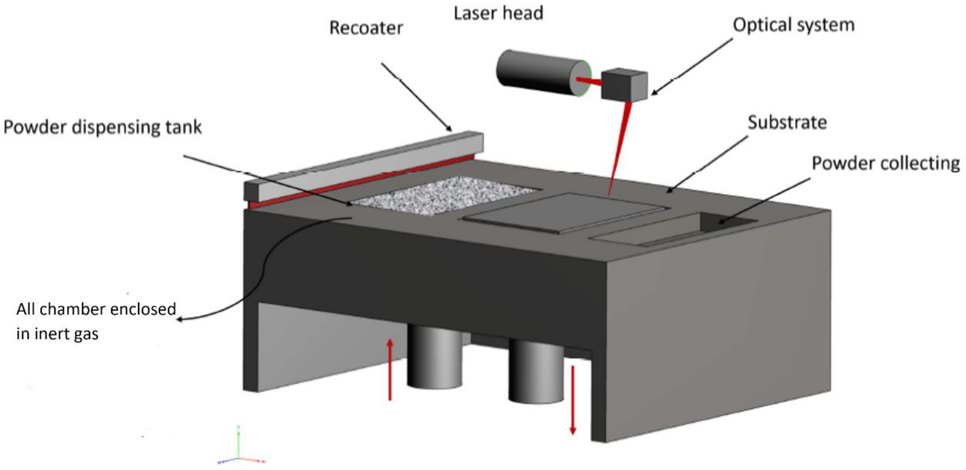
2. Overview of the L-PBF Process
2.1. Process Parameters
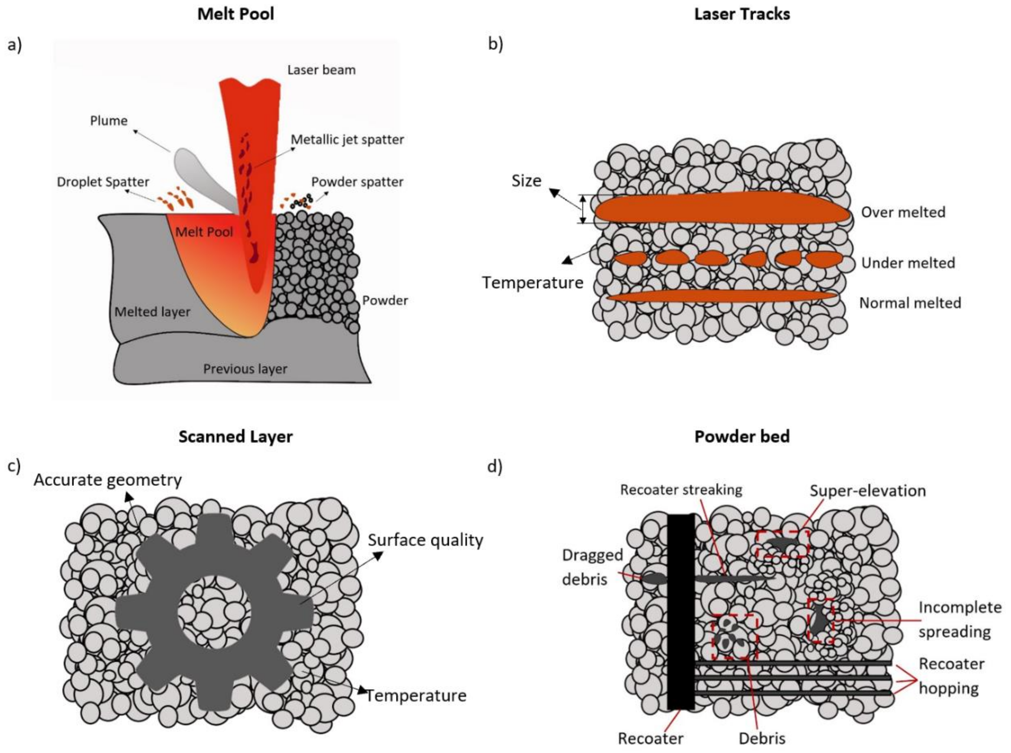
2.2. Process Signatures
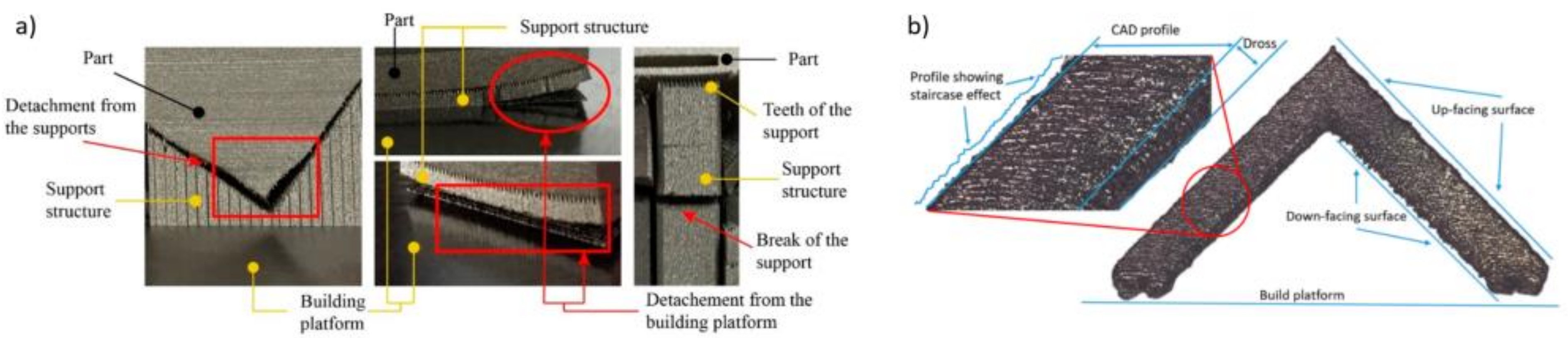
2.3. Defects
2.3.1. Dimensional Accuracy and Surface Quality
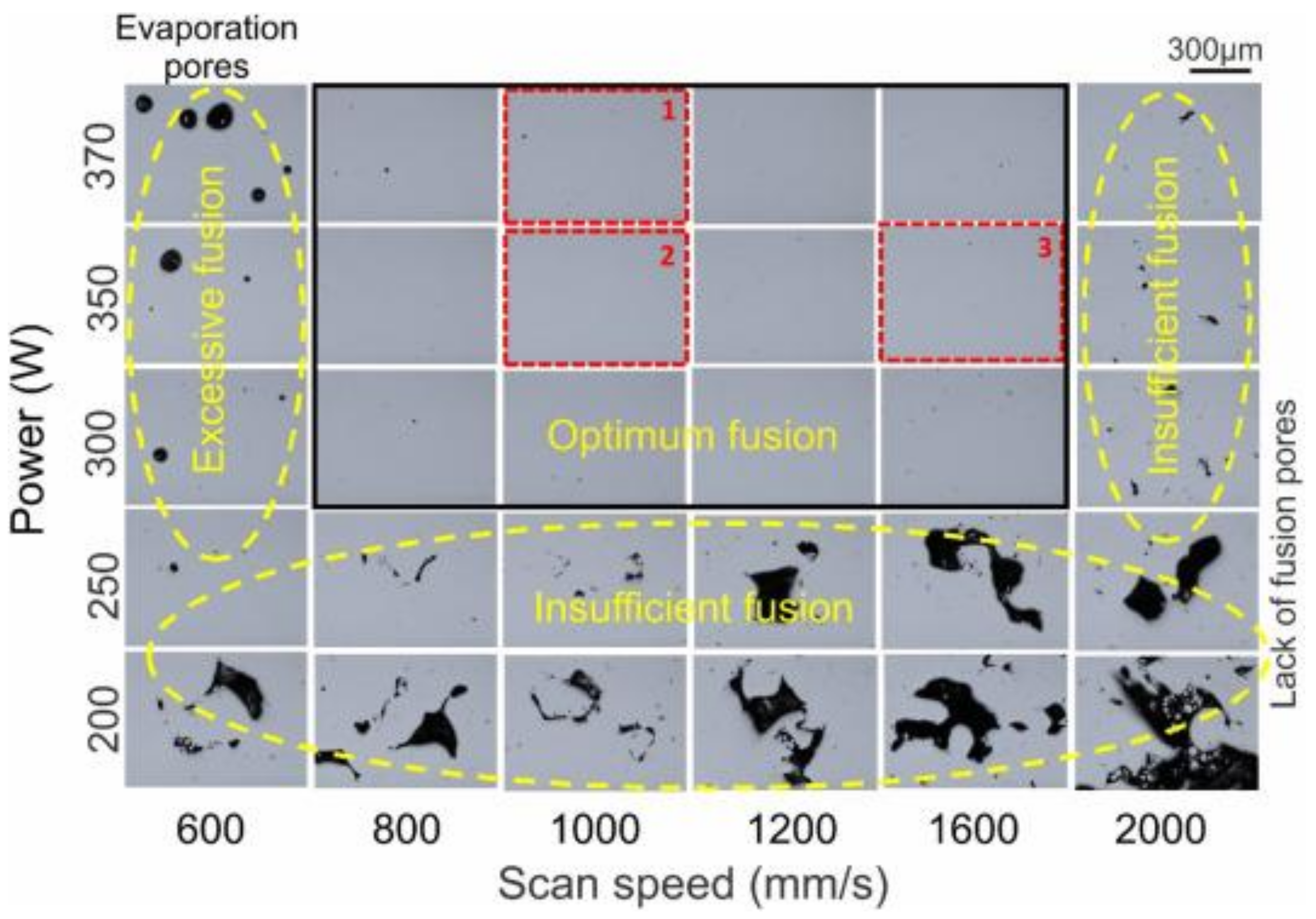
2.3.2. Porosity
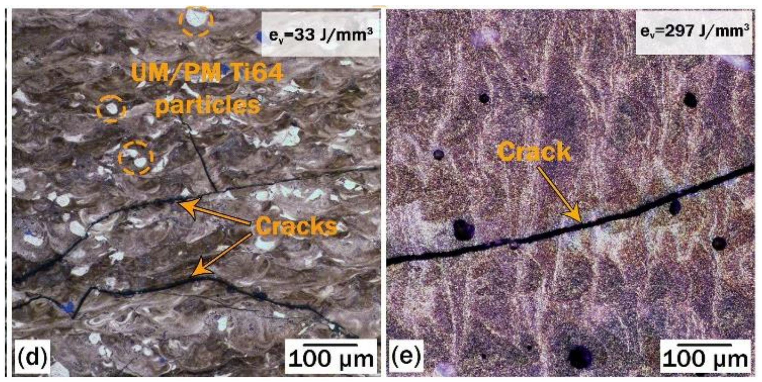
2.3.3. Thermally Induced Cracks
3. In Situ Sensors Used in the L-PBF Processes
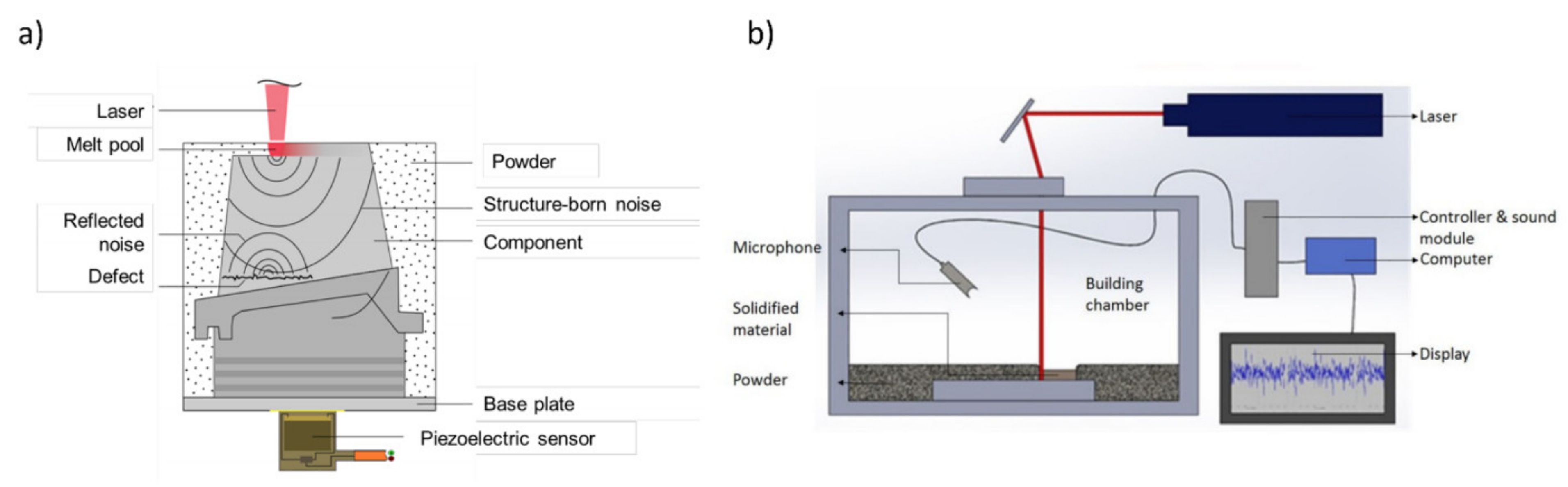
3.1. Acoustic Sensors
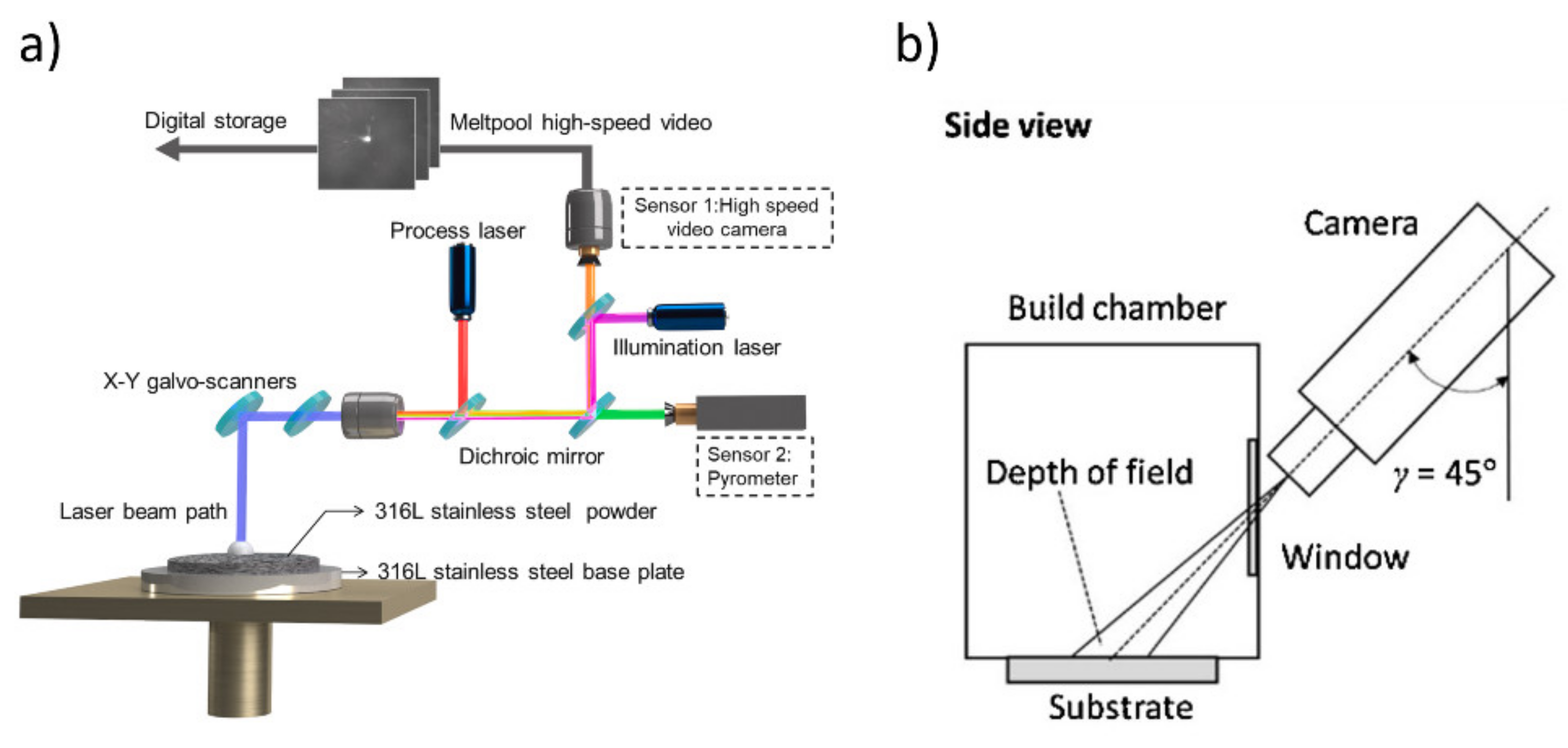
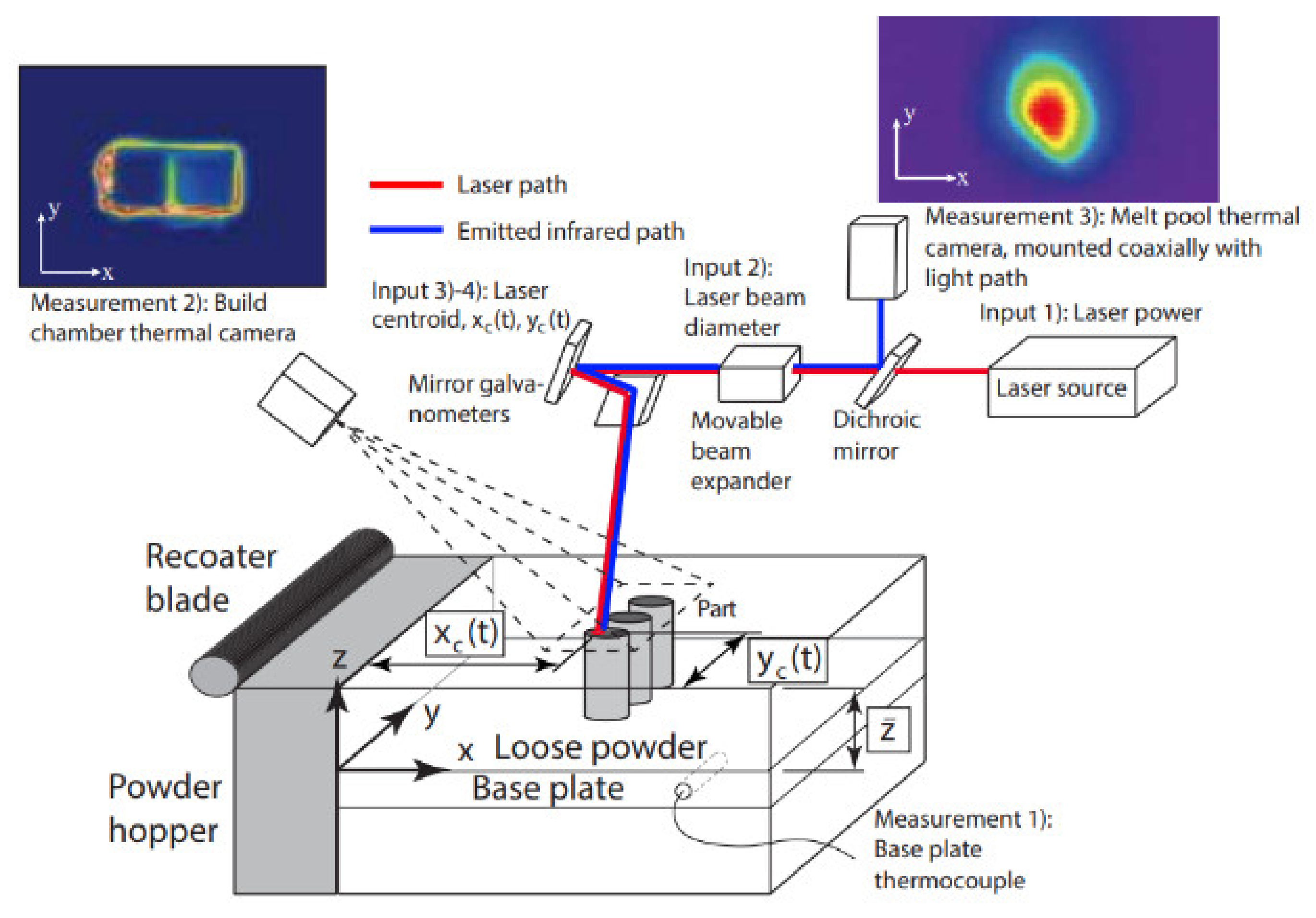
3.2. Vision Sensors
3.3. Temperature Sensors
4. ML Techniques
4.1. Data Preprocessing
4.2. Learning Approach
4.2.1. Supervised Learning
4.2.2. Unsupervised Learning
4.2.3. Semi-supervised Learning
4.2.4. Reinforcement Learning
4.3. Classification Performance Assessment
5. Defect Detection Using ML Techniques and Sensors
5.1. Acoustic Emission
5.2. Vision Sensor
5.3. Temperature Sensors
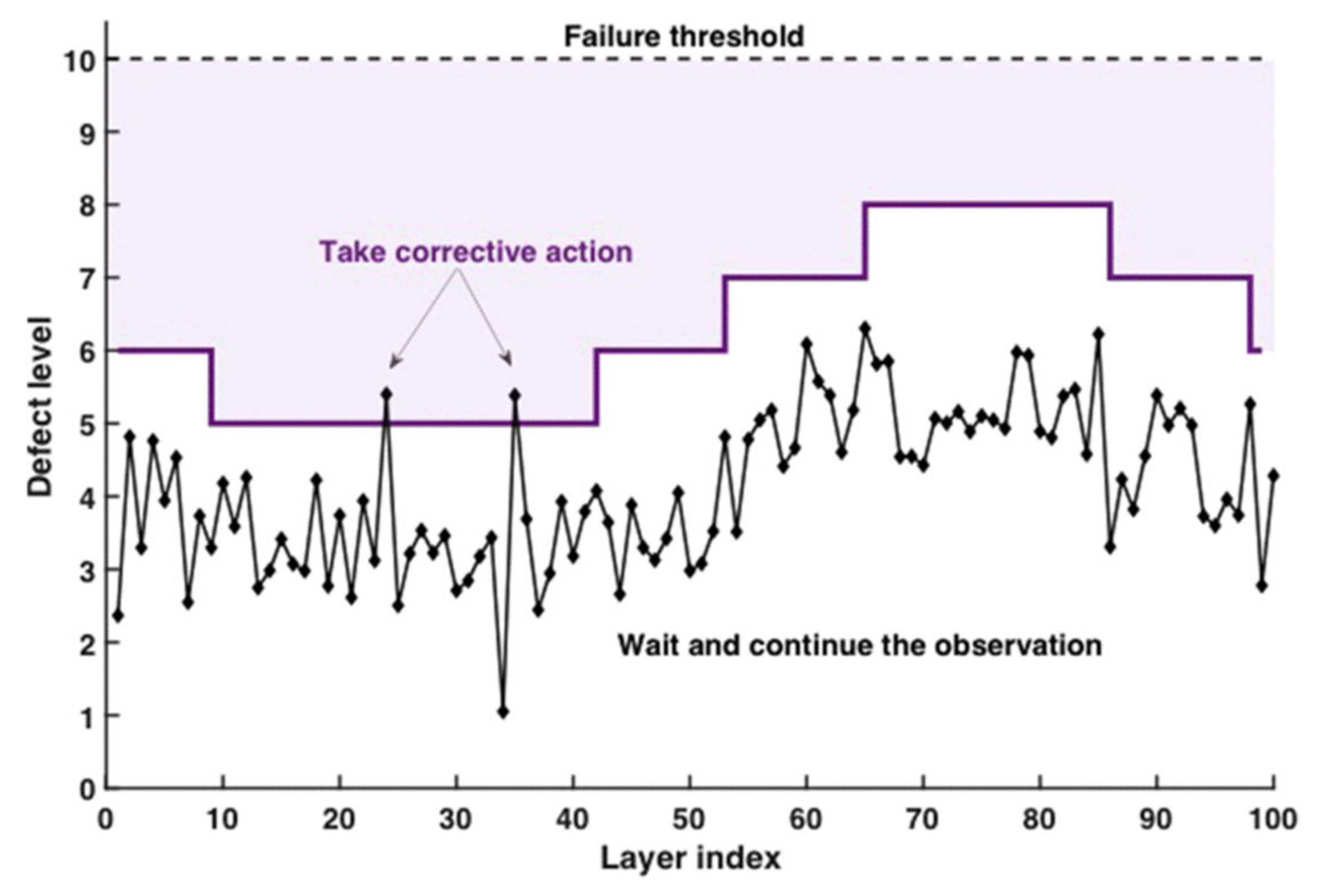
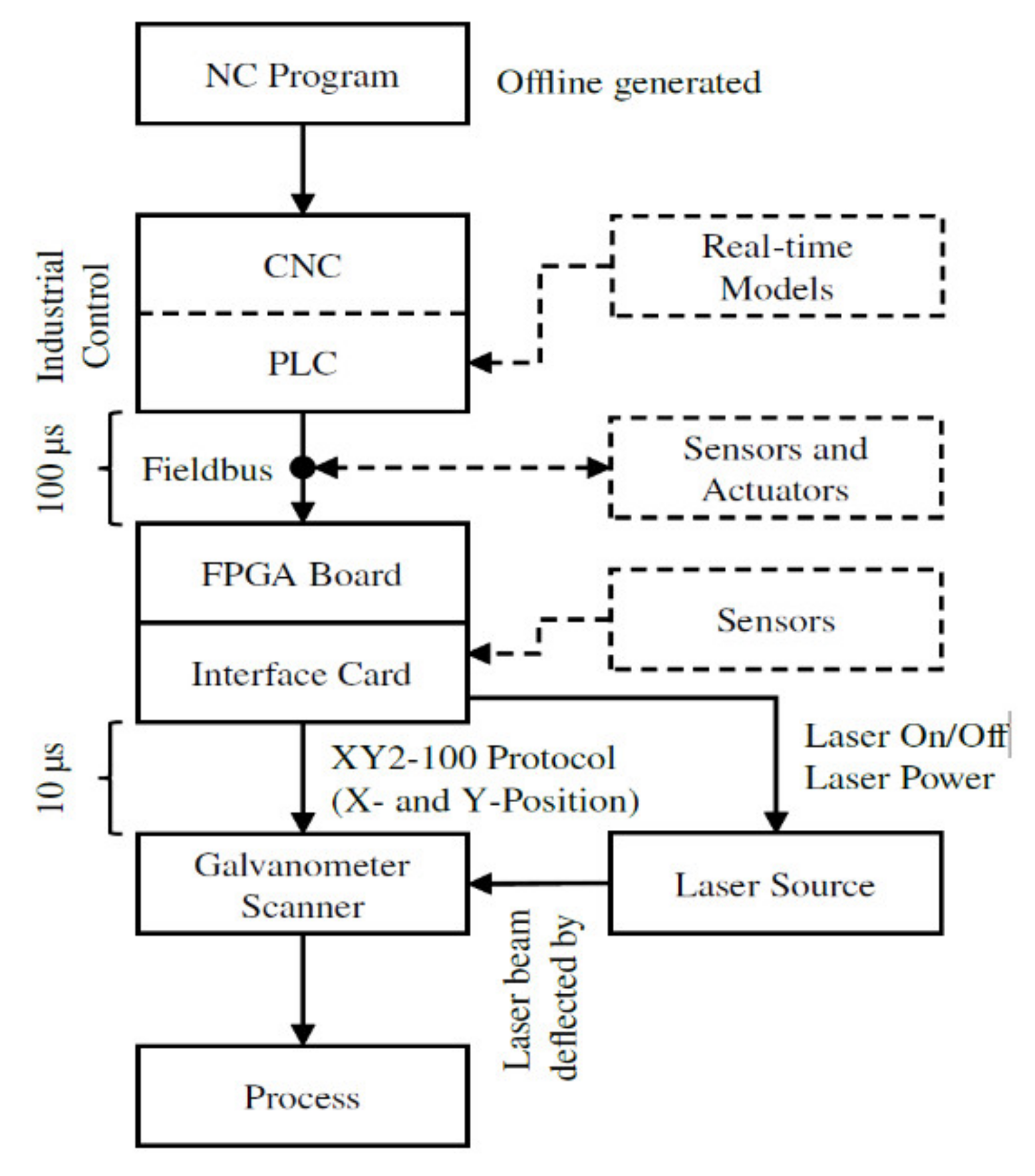
6. In-Process Control
7. Summary and Perspective
7.1. Data Volume, Velocity, and Variety
7.2. Generalization Issues
7.3. Sensor Fusion and Development
7.4. AM Framework Development
Author Contributions
Funding
Conflicts of Interest
References
- Dev Singh, D.; Mahender, T.; Raji Reddy, A. Powder bed fusion process: A brief review. Mater. Today Proc. 2021, 46, 350–355. [Google Scholar] [CrossRef]
- Khorasani, A.; Gibson, I.; Veetil, J.K.; Ghasemi, A.H. A review of technological improvements in laser-based powder bed fusion of metal printers. Int. J. Adv. Manuf. Technol. 2020, 108, 191–209. [Google Scholar] [CrossRef]
- Grasso, M.; Colosimo, B.M. Process defects and in situ monitoring methods in metal powder bed fusion: A review. Meas. Sci. Technol. 2017, 28, 044005. [Google Scholar] [CrossRef] [Green Version]
- Nazir, A.; Abate, K.M.; Kumar, A.; Jeng, J.-Y. A state-of-the-art review on types, design, optimization, and additive manufacturing of cellular structures. Int. J. Adv. Manuf. Technol. 2019, 104, 3489–3510. [Google Scholar] [CrossRef]
- Achillas, C.; Tzetzis, D.; Raimondo, M.O. Alternative production strategies based on the comparison of additive and traditional manufacturing technologies. Int. J. Prod. Res. 2017, 55, 3497–3509. [Google Scholar] [CrossRef]
- Thompson, M.K.; Moroni, G.; Vaneker, T.; Fadel, G.; Campbell, R.I.; Gibson, I.; Bernard, A.; Schulz, J.; Graf, P.; Ahuja, B.; et al. Design for Additive Manufacturing: Trends, opportunities, considerations, and constraints. CIRP Ann. 2016, 65, 737–760. [Google Scholar] [CrossRef] [Green Version]
- Mahmoud, D.; Elbestawi, M.A. Lattice Structures and Functionally Graded Materials Applications in Additive Manufacturing of Orthopedic Implants: A Review. J. Manuf. Mater. Process. 2017, 1, 13. [Google Scholar] [CrossRef]
- Jahan, S.A.; El-Mounayri, H. Optimal conformal cooling channels in 3D printed dies for plastic injection molding. Procedia Manuf. 2016, 5, 888–900. [Google Scholar] [CrossRef] [Green Version]
- Dowling, L.; Kennedy, J.; O’Shaughnessy, S.; Trimble, D. A review of critical repeatability and reproducibility issues in powder bed fusion. Mater. Des. 2020, 186, 108346. [Google Scholar] [CrossRef]
- Malekipour, E.; El-Mounayri, H. Common defects and contributing parameters in powder bed fusion AM process and their classification for online monitoring and control: A review. Int. J. Adv. Manuf. Technol. 2018, 95, 527–550. [Google Scholar] [CrossRef]
- DebRoy, T.; Wei, H.L.; Zuback, J.S.; Mukherjee, T.; Elmer, J.W.; Milewski, J.O.; Beese, A.M.; Wilson-Heid, A.; De, A.; Zhang, W. Additive manufacturing of metallic components—Process, structure and properties. Prog. Mater. Sci. 2018, 92, 112–224. [Google Scholar] [CrossRef]
- Zhang, J.; Song, B.; Wei, Q.; Bourell, D.; Shi, Y. A review of selective laser melting of aluminum alloys: Processing, microstructure, property and developing trends. J. Mater. Sci. Technol. 2019, 35, 270–284. [Google Scholar] [CrossRef]
- Shipley, H.; McDonnell, D.; Culleton, M.; Coull, R.; Lupoi, R.; O’Donnell, G.; Trimble, D. Optimisation of process parameters to address fundamental challenges during selective laser melting of Ti-6Al-4V: A review. Int. J. Mach. Tools Manuf. 2018, 128, 1–20. [Google Scholar] [CrossRef]
- Frazier, W.E. Metal Additive Manufacturing: A Review. J. Mater. Eng. Perform. 2014, 23, 1917–1928. [Google Scholar] [CrossRef]
- Sames, W.J.; List, F.A.; Pannala, S.; Dehoff, R.R.; Babu, S.S. The metallurgy and processing science of metal additive manufacturing. Int. Mater. Rev. 2016, 61, 315–360. [Google Scholar] [CrossRef]
- King, W.; Anderson, A.T.; Ferencz, R.M.; Hodge, N.E.; Kamath, C.; Khairallah, S.A. Overview of modelling and simulation of metal powder bed fusion process at Lawrence Livermore National Laboratory. Mater. Sci. Technol. 2015, 31, 957–968. [Google Scholar] [CrossRef]
- Zeng, K.; Pal, D.; Stucker, B. A review of thermal analysis methods in Laser Sintering and Selective Laser Melting. In Proceedings of the 2012 International Solid Freeform Fabrication Symposium, Austin, TX, USA, 6–8 August 2012; p. 19. [Google Scholar]
- Francois, M.M.; Sun, A.; King, W.E.; Henson, N.J.; Tourret, D.; Bronkhorst, C.A.; Carlson, N.N.; Newman, C.K.; Haut, T.; Bakosi, J.; et al. Modeling of additive manufacturing processes for metals: Challenges and opportunities. Curr. Opin. Solid State Mater. Sci. 2017, 21, 198–206. [Google Scholar] [CrossRef]
- Meng, L.; McWilliams, B.; Jarosinski, W.; Park, H.-Y.; Jung, Y.-G.; Lee, J.; Zhang, J. Machine Learning in Additive Manufacturing: A Review. JOM 2020, 72, 2363–2377. [Google Scholar] [CrossRef]
- Everton, S.K.; Hirsch, M.; Stravroulakis, P.; Leach, R.K.; Clare, A.T. Review of in-situ process monitoring and in-situ metrology for metal additive manufacturing. Mater. Des. 2016, 95, 431–445. [Google Scholar] [CrossRef]
- Reiff, C.; Bubeck, W.; Krawczyk, D.; Steeb, M.; Lechler, A.; Verl, A. Learning Feedforward Control for Laser Powder Bed Fusion. Procedia CIRP 2021, 96, 127–132. [Google Scholar] [CrossRef]
- Razvi, S.S.; Feng, S.; Narayanan, A.; Lee, Y.-T.T.; Witherell, P. A Review of Machine Learning Applications in Additive Manufacturing. In Proceedings of the Volume 1: 39th Computers and Information in Engineering Conference, Anaheim, CA, USA, 18–21 August 2019; American Society of Mechanical Engineers: New York, NY, USA, 2019; p. V001T02A040. [Google Scholar]
- Wuest, T.; Weimer, D.; Irgens, C.; Thoben, K.-D. Machine learning in manufacturing: Advantages, challenges, and applications. Prod. Manuf. Res. 2016, 4, 23–45. [Google Scholar] [CrossRef] [Green Version]
- Syafrudin, M.; Alfian, G.; Fitriyani, N.L.; Rhee, J. Performance Analysis of IoT-Based Sensor, Big Data Processing, and Machine Learning Model for Real-Time Monitoring System in Automotive Manufacturing. Sensors 2018, 18, 2946. [Google Scholar] [CrossRef] [Green Version]
- Dogan, A.; Birant, D. Machine learning and data mining in manufacturing. Expert Syst. Appl. 2021, 166, 114060. [Google Scholar] [CrossRef]
- Yadav, P.; Rigo, O.; Arvieu, C.; Le Guen, E.; Lacoste, E. In Situ Monitoring Systems of The SLM Process: On the Need to Develop Machine Learning Models for Data Processing. Crystals 2020, 10, 524. [Google Scholar] [CrossRef]
- Wang, C.; Tan, X.P.; Tor, S.B.; Lim, C.S. Machine learning in additive manufacturing: State-of-the-art and perspectives. Addit. Manuf. 2020, 36, 101538. [Google Scholar] [CrossRef]
- Huang, D.J.; Li, H. A machine learning guided investigation of quality repeatability in metal laser powder bed fusion additive manufacturing. Mater. Des. 2021, 203, 109606. [Google Scholar] [CrossRef]
- Yap, C.Y.; Chua, C.K.; Dong, Z.L.; Liu, Z.H.; Zhang, D.Q.; Loh, L.E.; Sing, S.L. Review of selective laser melting: Materials and applications. Appl. Phys. Rev. 2015, 2, 041101. [Google Scholar] [CrossRef]
- Beitz, S.; Uerlich, R.; Bokelmann, T.; Diener, A.; Vietor, T.; Kwade, A. Influence of Powder Deposition on Powder Bed and Specimen Properties. Materials 2019, 12, 297. [Google Scholar] [CrossRef] [Green Version]
- Daňa, M.; Zetková, I.; Hanzl, P. The Influence of a Ceramic Recoater Blade on 3D Printing using Direct Metal Laser Sintering. Manuf. Technol. 2019, 19, 23–28. [Google Scholar] [CrossRef]
- Sola, A.; Nouri, A. Microstructural porosity in additive manufacturing: The formation and detection of pores in metal parts fabricated by powder bed fusion. J. Adv. Manuf. Process. 2019, 1, e10021. [Google Scholar] [CrossRef]
- Mani, M.; Lane, B.; Donmez, A.; Feng, S.; Moylan, S.; Fesperman, R. Measurement Science Needs for Real-Time Control of Additive Manufacturing Powder Bed Fusion Processes; NIST IR 8036; National Institute of Standards and Technology: Gaithersburg, MD, USA, 2015. [Google Scholar]
- Spears, T.G.; Gold, S.A. In-process sensing in selective laser melting (SLM) additive manufacturing. Integr. Mater. Manuf. Innov. 2016, 5, 16–40. [Google Scholar] [CrossRef] [Green Version]
- Grasso, M.; Colosimo, B.M. A statistical learning method for image-based monitoring of the plume signature in laser powder bed fusion. Robot. Comput.-Integr. Manuf. 2019, 57, 103–115. [Google Scholar] [CrossRef]
- Tenbrock, C.; Kelliger, T.; Praetzsch, N.; Ronge, M.; Jauer, L.; Schleifenbaum, J.H. Effect of laser-plume interaction on part quality in multi-scanner Laser Powder Bed Fusion. Addit. Manuf. 2021, 38, 101810. [Google Scholar] [CrossRef]
- Wang, D.; Wu, S.; Fu, F.; Mai, S.; Yang, Y.; Liu, Y.; Song, C. Mechanisms and characteristics of spatter generation in SLM processing and its effect on the properties. Mater. Des. 2017, 117, 121–130. [Google Scholar] [CrossRef]
- Yadroitsev, I.; Gusarov, A.; Yadroitsava, I.; Smurov, I. Single track formation in selective laser melting of metal powders. J. Mater. Process. Technol. 2010, 210, 1624–1631. [Google Scholar] [CrossRef]
- Abdelrahman, M.; Reutzel, E.W.; Nassar, A.R.; Starr, T.L. Flaw detection in powder bed fusion using optical imaging. Addit. Manuf. 2017, 15, 1–11. [Google Scholar] [CrossRef]
- Calignano, F.; Lorusso, M.; Pakkanen, J.; Trevisan, F.; Ambrosio, E.P.; Manfredi, D.; Fino, P. Investigation of accuracy and dimensional limits of part produced in aluminum alloy by selective laser melting. Int. J. Adv. Manuf. Technol. 2017, 88, 451–458. [Google Scholar] [CrossRef]
- Shamsaei, N.; Yadollahi, A.; Bian, L.; Thompson, S.M. An overview of Direct Laser Deposition for additive manufacturing; Part II: Mechanical behavior, process parameter optimization and control. Addit. Manuf. 2015, 8, 12–35. [Google Scholar] [CrossRef]
- Hiren, M.; Gajera, M.E.; Dave, K.G.; Jani, V.P. Experimental investigation and analysis of dimensional accuracy of laser-based powder bed fusion made specimen by application of response surface methodology. Prog. Addit. Manuf. 2019, 4, 371–382. [Google Scholar] [CrossRef]
- Zhang, L.; Zhang, S.; Zhu, H. Effect of scanning strategy on geometric accuracy of the circle structure fabricated by selective laser melting. J. Manuf. Process. 2021, 64, 907–915. [Google Scholar] [CrossRef]
- Almabrouk Mousa, A. Experimental investigations of curling phenomenon in selective laser sintering process. Rapid Prototyp. J. 2016, 22, 405–415. [Google Scholar] [CrossRef]
- Calignano, F.; Minetola, P. Influence of Process Parameters on the Porosity, Accuracy, Roughness, and Support Structures of Hastelloy X Produced by Laser Powder Bed Fusion. Materials 2019, 12, 3178. [Google Scholar] [CrossRef] [Green Version]
- Kleszczynski, S.; zur Jacobsmühlen, J.; Sehrt, J.; Witt, G. Error detection in laser beam melting systems by high resolution imaging. In Proceedings of the Twenty Third Annual International Solid Freeform Fabrication Symposium, Austin, TX, USA, 6–8 August 2012; p. 987. [Google Scholar]
- Li, R.; Liu, J.; Shi, Y.; Wang, L.; Jiang, W. Balling behavior of stainless steel and nickel powder during selective laser melting process. Int. J. Adv. Manuf. Technol. 2012, 59, 1025–1035. [Google Scholar] [CrossRef]
- Kruth, J.P.; Froyen, L.; Van Vaerenbergh, J.; Mercelis, P.; Rombouts, M.; Lauwers, B. Selective laser melting of iron-based powder. J. Mater. Process. Technol. 2004, 149, 616–622. [Google Scholar] [CrossRef]
- Tang, C.; Le, K.Q.; Wong, C.H. Physics of humping formation in laser powder bed fusion. Int. J. Heat Mass Transf. 2020, 149, 119172. [Google Scholar] [CrossRef]
- Charles, A.; Elkaseer, A.; Thijs, L.; Hagenmeyer, V.; Scholz, S. Effect of Process Parameters on the Generated Surface Roughness of Down-Facing Surfaces in Selective Laser Melting. Appl. Sci. 2019, 9, 1256. [Google Scholar] [CrossRef] [Green Version]
- Charles, A.; Elkaseer, A.; Thijs, L.; Scholz, S.G. Dimensional Errors Due to Overhanging Features in Laser Powder Bed Fusion Parts Made of Ti-6Al-4V. Appl. Sci. 2020, 10, 2416. [Google Scholar] [CrossRef]
- Salmi, A.; Calignano, F.; Galati, M.; Atzeni, E. An integrated design methodology for components produced by laser powder bed fusion (L-PBF) process. Virtual Phys. Prototyp. 2018, 13, 191–202. [Google Scholar] [CrossRef]
- Kruth, J.-P.; Duflou, J.; Mercelis, P.; Van Vaerenbergh, J.; Craeghs, T.; De Keuster, J. On-line monitoring and process control in selective laser melting and laser cutting. In Proceedings of the 5th Lane Conference, Laser Assisted Net Shape Engineering, Erlangen, Germany, 25–28 September 2007; Volume 1, pp. 23–37. [Google Scholar]
- Hooper, P.A. Melt pool temperature and cooling rates in laser powder bed fusion. Addit. Manuf. 2018, 22, 548–559. [Google Scholar] [CrossRef]
- Bayat, M.; Thanki, A.; Mohanty, S.; Witvrouw, A.; Yang, S.; Thorborg, J.; Tiedje, N.S.; Hattel, J.H. Keyhole-induced porosities in Laser-based Powder Bed Fusion (L-PBF) of Ti6Al4V: High-fidelity modelling and experimental validation. Addit. Manuf. 2019, 30, 100835. [Google Scholar] [CrossRef]
- Sabzi, H.E.; Maeng, S.; Liang, X.; Simonelli, M.; Aboulkhair, N.T.; Rivera-Díaz-del-Castillo, P.E.J. Controlling crack formation and porosity in laser powder bed fusion: Alloy design and process optimisation. Addit. Manuf. 2020, 34, 101360. [Google Scholar] [CrossRef]
- Gordon, J.V.; Narra, S.P.; Cunningham, R.W.; Liu, H.; Chen, H.; Suter, R.M.; Beuth, J.L.; Rollett, A.D. Defect structure process maps for laser powder bed fusion additive manufacturing. Addit. Manuf. 2020, 36, 101552. [Google Scholar] [CrossRef]
- Tang, M.; Pistorius, P.C. Oxides, porosity and fatigue performance of AlSi10Mg parts produced by selective laser melting. Int. J. Fatigue 2017, 94, 192–201. [Google Scholar] [CrossRef]
- Bayoumy, D.; Schliephake, D.; Dietrich, S.; Wu, X.H.; Zhu, Y.M.; Huang, A.J. Intensive processing optimization for achieving strong and ductile Al-Mn-Mg-Sc-Zr alloy produced by selective laser melting. Mater. Des. 2021, 198, 109317. [Google Scholar] [CrossRef]
- Ng, G.K.L.; Jarfors, A.E.W.; Bi, G.; Zheng, H.Y. Porosity formation and gas bubble retention in laser metal deposition. Appl. Phys. A 2009, 97, 641–649. [Google Scholar] [CrossRef]
- Gong, H.; Rafi, K.; Gu, H.; Starr, T.; Stucker, B. Analysis of defect generation in Ti–6Al–4V parts made using powder bed fusion additive manufacturing processes. Addit. Manuf. 2014, 1–4, 87–98. [Google Scholar] [CrossRef]
- Zhang, B.; Li, Y.; Bai, Q. Defect Formation Mechanisms in Selective Laser Melting: A Review. Chin. J. Mech. Eng. 2017, 30, 515–527. [Google Scholar] [CrossRef] [Green Version]
- Promoppatum, P.; Yao, S.-C. Analytical evaluation of defect generation for selective laser melting of metals. Int. J. Adv. Manuf. Technol. 2019, 103, 1185–1198. [Google Scholar] [CrossRef]
- Wang, W.; Ning, J.; Liang, S.Y. Prediction of lack-of-fusion porosity in laser powder-bed fusion considering boundary conditions and sensitivity to laser power absorption. Int. J. Adv. Manuf. Technol. 2021, 112, 61–70. [Google Scholar] [CrossRef]
- Tang, M.; Pistorius, P.C.; Beuth, J.L. Prediction of lack-of-fusion porosity for powder bed fusion. Addit. Manuf. 2017, 14, 39–48. [Google Scholar] [CrossRef]
- King, W.E.; Barth, H.D.; Castillo, V.M.; Gallegos, G.F.; Gibbs, J.W.; Hahn, D.E.; Kamath, C.; Rubenchik, A.M. Observation of keyhole-mode laser melting in laser powder-bed fusion additive manufacturing. J. Mater. Process. Technol. 2014, 214, 2915–2925. [Google Scholar] [CrossRef]
- Paulson, N.H.; Gould, B.; Wolff, S.J.; Stan, M.; Greco, A.C. Correlations between thermal history and keyhole porosity in laser powder bed fusion. Addit. Manuf. 2020, 34, 101213. [Google Scholar] [CrossRef]
- Mercelis, P.; Kruth, J.-P. Residual stresses in selective laser sintering and selective laser melting. Rapid Prototyp. J. 2006, 12, 254–265. [Google Scholar] [CrossRef]
- Vrancken, B. Study of Residual Stresses in Selective Laser Melting. 2016. Available online: https://lirias.kuleuven.be/1942277 (accessed on 20 April 2021).
- Fereiduni, E.; Ghasemi, A.; Elbestawi, M.; Dinkar Jadhav, S.; Vanmeensel, K. Laser Powder Bed Fabrication of Nickel-base Superalloys: Influence of Parameters; Characterisation, Quantification and Mitigation of Cracking. Superalloys 2012, 2012, 2826–2834. [Google Scholar]
- Alimardani, M.; Toyserkani, E.; Huissoon, J.P.; Paul, C.P. On the delamination and crack formation in a thin wall fabricated using laser solid freeform fabrication process: An experimental–numerical investigation. Opt. Lasers Eng. 2009, 47, 1160–1168. [Google Scholar] [CrossRef]
- Yakout, M.; Phillips, I.; Elbestawi, M.A.; Fang, Q. In-situ monitoring and detection of spatter agglomeration and delamination during laser-based powder bed fusion of Invar 36. Opt. Laser Technol. 2020, 136, 106741. [Google Scholar] [CrossRef]
- Mohammadi, M.G.; Mahmoud, D.; Elbestawi, M. On the application of machine learning for defect detection in L-PBF additive manufacturing. Opt. Laser Technol. 2021, 143, 107338. [Google Scholar] [CrossRef]
- Fereiduni, E.; Ghasemi, A.; Elbestawi, M.; Jadhav, S.D.; Vanmeensel, K. Laser powder bed fusion processability of Ti-6Al-4V powder decorated by B4C particles. Mater. Lett. 2021, 296, 129923. [Google Scholar] [CrossRef]
- Ohtsu, M. Acoustic Emission and Related Non-Destructive Evaluation Techniques in the Fracture Mechanics of Concrete: Fundamentals and Applications; Woodhead Publishing: Sawston, UK, 2020; ISBN 978-0-12-823514-0. [Google Scholar]
- Sharma, A.; Junaidh, M.; Purushothaman, K.; Kotwal, C.; Paul, J.; Tripathi, S.; Pant, B.; Sankaranarayanan, A. Online Monitoring of Electron Beam Welding of TI6AL4V Alloy Through Acoustic Emission. In Proceedings of the National Seminar on Non-Destructive Evaluation, Hyderabad, India, 7–9 December 2006. [Google Scholar]
- Beattie, A. Acoustic Emission Non-Destructive Testing of Structures Using Source Location Techniques; SAND2013-7779; Sandia National Lab. (SNL-NM): Albuquerque, NM, USA, 2013; p. 1096442. [Google Scholar]
- Eschner, N.; Weiser, L.; Häfner, B.; Lanza, G. Classification of specimen density in Laser Powder Bed Fusion (L-PBF) using in-process structure-borne acoustic process emissions. Addit. Manuf. 2020, 34, 101324. [Google Scholar] [CrossRef]
- Kageyama, K.; Murayama, H.; Ohsawa, I.; Kanai, M.; Nagata, K.; Machijima, Y.; Matsumura, F. Acoustic emission monitoring of a reinforced concrete structure by applying new fiber-optic sensors. Smart Mater. Struct. 2005, 14, S52–S59. [Google Scholar] [CrossRef]
- Eschner, N.; Weiser, L.; Häfner, B.; Lanza, G. Development of an acoustic process monitoring system for selective laser melting (SLM). In Proceedings of the 29th Annual International Solid Freeform Fabrication Symposium, Austin, TX, USA, 13–15 August 2018; pp. 13–15. [Google Scholar]
- Kouprianoff, D.; Luwes, N.; Yadroitsava, I.; Yadroitsev, I. Acoustic Emission Technique for Online Detection of Fusion Defects for Single Tracks during Metal Laser Powder Bed Fusion. In Proceedings of the 2018 International Solid Freeform Fabrication Symposium, Austin, TX, USA, 13–15 August 2018; p. 10. [Google Scholar]
- Kwon, O.; Kim, H.G.; Ham, M.J.; Kim, W.; Kim, G.-H.; Cho, J.-H.; Kim, N.I.; Kim, K. A deep neural network for classification of melt-pool images in metal additive manufacturing. J. Intell. Manuf. 2020, 31, 375–386. [Google Scholar] [CrossRef]
- Ye, D.; Hsi Fuh, J.Y.; Zhang, Y.; Hong, G.S.; Zhu, K. In situ monitoring of selective laser melting using plume and spatter signatures by deep belief networks. ISA Trans. 2018, 81, 96–104. [Google Scholar] [CrossRef]
- Nakamura, J. Image Sensors and Signal Processing for Digital Still Cameras; CRC Press: Boca Raton, FL, USA, 2017; ISBN 978-1-4200-2685-6. [Google Scholar]
- Gobert, C.; Reutzel, E.W.; Petrich, J.; Nassar, A.R.; Phoha, S. Application of supervised machine learning for defect detection during metallic powder bed fusion additive manufacturing using high resolution imaging. Addit. Manuf. 2018, 21, 517–528. [Google Scholar] [CrossRef]
- Repossini, G.; Laguzza, V.; Grasso, M.; Colosimo, B.M. On the use of spatter signature for in-situ monitoring of Laser Powder Bed Fusion. Addit. Manuf. 2017, 16, 35–48. [Google Scholar] [CrossRef]
- Caltanissetta, F.; Grasso, M.; Petrò, S.; Colosimo, B.M. Characterization of in-situ measurements based on layerwise imaging in laser powder bed fusion. Addit. Manuf. 2018, 24, 183–199. [Google Scholar] [CrossRef]
- Masoomi, M.; Thompson, S.M.; Shamsaei, N. Laser powder bed fusion of Ti-6Al-4V parts: Thermal modeling and mechanical implications. Int. J. Mach. Tools Manuf. 2017, 118–119, 73–90. [Google Scholar] [CrossRef] [Green Version]
- Khan, K.; Mohr, G.; Hilgenberg, K.; De, A. Probing a novel heat source model and adaptive remeshing technique to simulate laser powder bed fusion with experimental validation. Comput. Mater. Sci. 2020, 181, 109752. [Google Scholar] [CrossRef]
- Craeghs, T.; Clijsters, S.; Kruth, J.-P.; Bechmann, F.; Ebert, M.-C. Detection of Process Failures in Layerwise Laser Melting with Optical Process Monitoring. Phys. Procedia 2012, 39, 753–759. [Google Scholar] [CrossRef] [Green Version]
- Lane, B.; Whitenton, E.; Moylan, S. Multiple sensor detection of process phenomena in laser powder bed fusion. In Proceedings of the Thermosense: Thermal Infrared Applications XXXVIII, Baltimore, MD, USA, 18–24 April 2016; International Society for Optics and Photonics: Bellingham, WA, USA, 2016; Volume 9861, p. 986104. [Google Scholar]
- Lough, C.S.; Escano, L.I.; Qu, M.; Smith, C.C.; Landers, R.G.; Bristow, D.A.; Chen, L.; Kinzel, E.C. In-situ optical emission spectroscopy of selective laser melting. J. Manuf. Process. 2020, 53, 336–341. [Google Scholar] [CrossRef]
- Dunbar, A.J.; Nassar, A.R. Assessment of optical emission analysis for in-process monitoring of powder bed fusion additive manufacturing. Virtual Phys. Prototyp. 2018, 13, 14–19. [Google Scholar] [CrossRef]
- Piili, H.; Lehti, A.; Taimisto, L.; Salminen, A.; Nyrhilä, O. Evaluation of Different Monitoring Methods of Laser Assisted Additive Manufacturing of Stainless Steel. In Proceedings of the 12th Conference of the European Ceramic Society, Stockholm, Sweden, 19–23 June 2011. [Google Scholar]
- Wood, N.; Hoelzle, D. Temperature states in Powder Bed Fusion additive manufacturing are structurally controllable and observable. arXiv 2020, arXiv:2001.02519. [Google Scholar]
- Dhall, D.; Kaur, R.; Juneja, M. Machine Learning: A Review of the Algorithms and Its Applications. In Proceedings of the ICRIC 2019; Singh, P.K., Kar, A.K., Singh, Y., Kolekar, M.H., Tanwar, S., Eds.; Springer International Publishing: Cham, Switzerland, 2020; pp. 47–63. [Google Scholar]
- Paturi, U.M.R.; Cheruku, S. Application and performance of machine learning techniques in manufacturing sector from the past two decades: A review. Mater. Today Proc. 2020, 38, 2392–2401. [Google Scholar] [CrossRef]
- Kotsiantis, S.B.; Kanellopoulos, D.; Pintelas, P.E. Data Preprocessing for Supervised Leaning Abstract. Int. J. Comput. Sci. 2006, 1, 111–117. [Google Scholar]
- Karpuschewski, B.; Wehmeier, M.; Inasaki, I. Grinding Monitoring System Based on Power and Acoustic Emission Sensors. CIRP Ann. 2000, 49, 235–240. [Google Scholar] [CrossRef]
- Mahato, V.; Obeidi, M.A.; Brabazon, D.; Cunningham, P. Detecting voids in 3D printing using melt pool time series data. J. Intell. Manuf. 2020, 1–8. [Google Scholar] [CrossRef]
- Scime, L.; Beuth, J. Using machine learning to identify in-situ melt pool signatures indicative of flaw formation in a laser powder bed fusion additive manufacturing process. Addit. Manuf. 2019, 25, 151–165. [Google Scholar] [CrossRef]
- Qi, X.; Chen, G.; Li, Y.; Cheng, X.; Li, C. Applying Neural-Network-Based Machine Learning to Additive Manufacturing: Current Applications, Challenges, and Future Perspectives. Engineering 2019, 5, 721–729. [Google Scholar] [CrossRef]
- Mohammed, M.; Khan, M.B.; Bashier, E.B.M. Machine Learning: Algorithms and Applications; CRC Press: Boca Raton, FL, USA, 2016; ISBN 978-1-4987-0539-4. [Google Scholar]
- Sarker, I.H.; Kayes, A.S.M.; Badsha, S.; Alqahtani, H.; Watters, P.; Ng, A. Cybersecurity data science: An overview from machine learning perspective. J. Big Data 2020, 7, 41. [Google Scholar] [CrossRef]
- Baumgartl, H.; Tomas, J.; Buettner, R.; Merkel, M. A deep learning-based model for defect detection in laser-powder bed fusion using in-situ thermographic monitoring. Prog. Addit. Manuf. 2020, 5, 277–285. [Google Scholar] [CrossRef] [Green Version]
- Hansson, K.; Yella, S.; Dougherty, M.; Fleyeh, H. Machine Learning Algorithms in Heavy Process Manufacturing. Am. J. Intell. Syst. 2016, 6, 1–13. [Google Scholar]
- Quality Prediction in Interlinked Manufacturing Processes based on Supervised & Unsupervised Machine Learning. Procedia CIRP 2013, 7, 193–198.
- Pandiyan, V.; Drissi-Daoudi, R.; Shevchik, S.; Masinelli, G.; Logé, R.; Wasmer, K. Analysis of time, frequency and time-frequency domain features from acoustic emissions during Laser Powder-Bed fusion process. Procedia CIRP 2020, 94, 392–397. [Google Scholar] [CrossRef]
- Kingma, D.P.; Rezende, D.J.; Mohamed, S.; Welling, M. Semi-Supervised Learning with Deep Generative Models. arXiv 2014, arXiv:1406.5298. [Google Scholar]
- Okaro, I.A.; Jayasinghe, S.; Sutcliffe, C.; Black, K.; Paoletti, P.; Green, P.L. Automatic fault detection for laser powder-bed fusion using semi-supervised machine learning. Addit. Manuf. 2019, 27, 42–53. [Google Scholar] [CrossRef]
- Sutton, R.S. Introduction: The Challenge of Reinforcement Learning. In Reinforcement Learning; Sutton, R.S., Ed.; The Springer International Series in Engineering and Computer Science; Springer: Boston, MA, USA, 1992; pp. 1–3. ISBN 978-1-4615-3618-5. [Google Scholar]
- Arulkumaran, K.; Deisenroth, M.P.; Brundage, M.; Bharath, A.A. Deep Reinforcement Learning: A Brief Survey. IEEE Signal Process. Mag. 2017, 34, 26–38. [Google Scholar] [CrossRef] [Green Version]
- Sarker, I.H. Machine Learning: Algorithms, Real-World Applications and Research Directions. SN Comput. Sci. 2021, 2, 160. [Google Scholar] [CrossRef]
- Wasmer, K.; Le-Quang, T.; Meylan, B.; Shevchik, S.A. In situ quality monitoring in AM using acoustic emission: A reinforcement learning approach. J. Mater. Eng. Perform. 2019, 28, 666–672. [Google Scholar] [CrossRef]
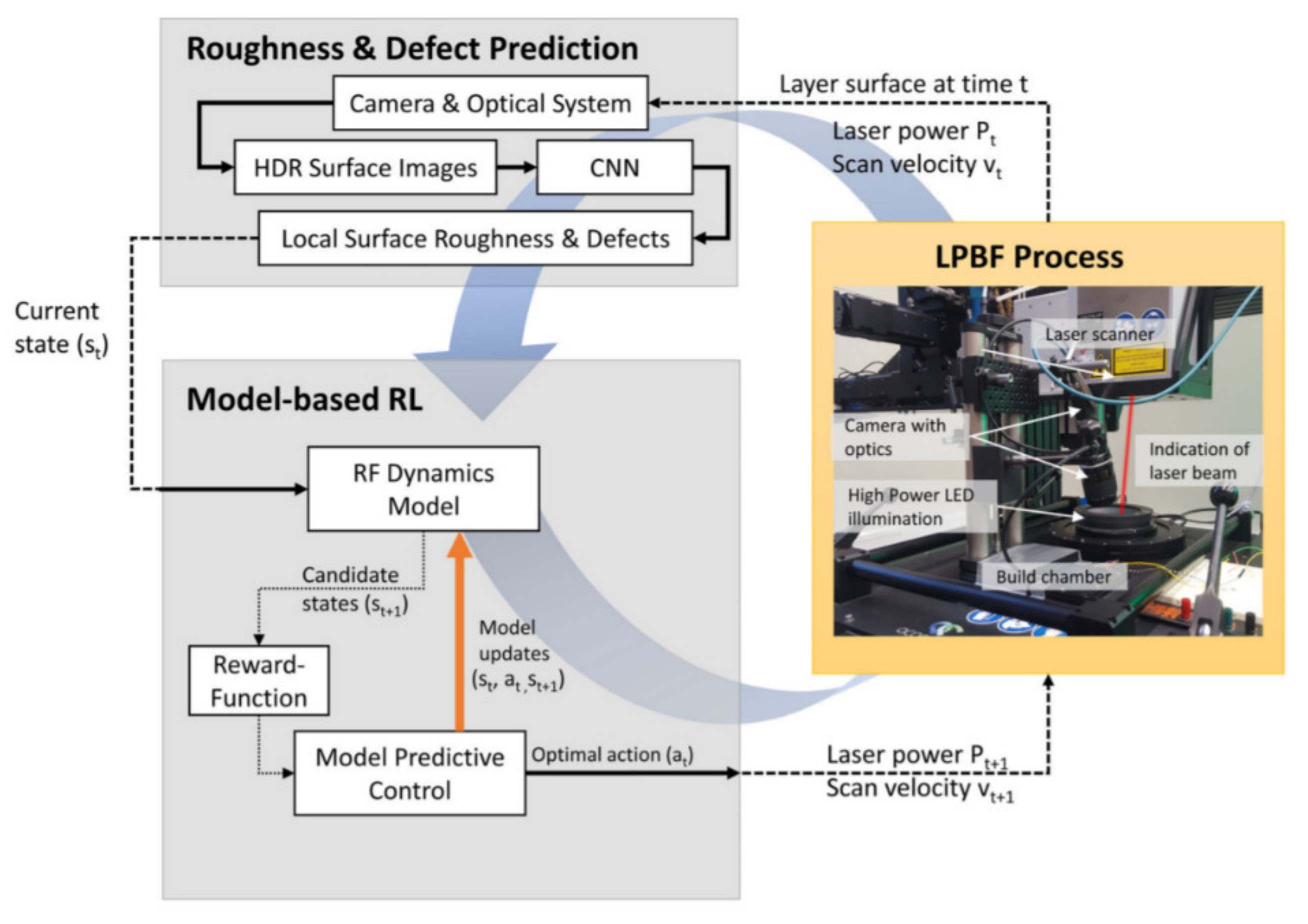
- Knaak, C.; Masseling, L.; Duong, E.; Abels, P.; Gillner, A. Improving Build Quality in Laser Powder Bed Fusion Using High Dynamic Range Imaging and Model-Based Reinforcement Learning. IEEE Access 2021, 9, 55214–55231. [Google Scholar] [CrossRef]
- García, V.; Mollineda, R.A.; Sánchez, J.S. A bias correction function for classification performance assessment in two-class imbalanced problems. Knowl.-Based Syst. 2014, 59, 66–74. [Google Scholar] [CrossRef]
- Saad, E.; Wang, H.; Kovacevic, R. Classification of molten pool modes in variable polarity plasma arc welding based on acoustic signature. J. Mater. Process. Technol. 2006, 174, 127–136. [Google Scholar] [CrossRef]
- Ye, D.; Hong, G.S.; Zhang, Y.; Zhu, K.; Fuh, J.Y.H. Defect detection in selective laser melting technology by acoustic signals with deep belief networks. Int. J. Adv. Manuf. Technol. 2018, 96, 2791–2801. [Google Scholar] [CrossRef]
- Wasmer, K.; Kenel, C.; Leinenbach, C.; Shevchik, S.A. In Situ and Real-Time Monitoring of Powder-Bed AM by Combining Acoustic Emission and Artificial Intelligence. In Industrializing Additive Manufacturing—Proceedings of Additive Manufacturing in Products and Applications—AMPA2017; Meboldt, M., Klahn, C., Eds.; Springer International Publishing: Cham, Switzerland, 2018; pp. 200–209. [Google Scholar]
- Shevchik, S.A.; Kenel, C.; Leinenbach, C.; Wasmer, K. Acoustic emission for in situ quality monitoring in additive manufacturing using spectral convolutional neural networks. Addit. Manuf. 2018, 21, 598–604. [Google Scholar] [CrossRef]
- Mohammadi, M.G.; Elbestawi, M. Real Time Monitoring in L-PBF Using a Machine Learning Approach. Procedia Manuf. 2020, 51, 725–731. [Google Scholar] [CrossRef]
- Shevchik, S.A.; Masinelli, G.; Kenel, C.; Leinenbach, C.; Wasmer, K. Deep Learning for In Situ and Real-Time Quality Monitoring in Additive Manufacturing Using Acoustic Emission. IEEE Trans. Ind. Inform. 2019, 15, 5194–5203. [Google Scholar] [CrossRef]
- Scime, L.; Beuth, J. Anomaly detection and classification in a laser powder bed additive manufacturing process using a trained computer vision algorithm. Addit. Manuf. 2018, 19, 114–126. [Google Scholar] [CrossRef]
- Imani, F.; Gaikwad, A.; Montazeri, M.; Rao, P.; Yang, H.; Reutzel, E. Process Mapping and In-Process Monitoring of Porosity in Laser Powder Bed Fusion Using Layerwise Optical Imaging. J. Manuf. Sci. Eng. 2018, 140, 101009. [Google Scholar] [CrossRef]
- Snow, Z.; Diehl, B.; Reutzel, E.W.; Nassar, A. Toward in-situ flaw detection in laser powder bed fusion additive manufacturing through layerwise imagery and machine learning. J. Manuf. Syst. 2021, 59, 12–26. [Google Scholar] [CrossRef]
- Aminzadeh, M.; Kurfess, T.R. Online quality inspection using Bayesian classification in powder-bed additive manufacturing from high-resolution visual camera images. J. Intell. Manuf. 2019, 30, 2505–2523. [Google Scholar] [CrossRef]
- Imani, F.; Chen, R.; Diewald, E.; Reutzel, E.; Yang, H. Deep learning of variant geometry in layerwise imaging profiles for additive manufacturing quality control. J. Manuf. Sci. Eng. 2019, 141, 111001. [Google Scholar] [CrossRef]
- Gaikwad, A.; Imani, F.; Yang, H.; Reutzel, E.; Rao, P. In Situ Monitoring of Thin-Wall Build Quality in Laser Powder Bed Fusion Using Deep Learning. Smart Sustain. Manuf. Syst. 2019, 3, 20190027. [Google Scholar] [CrossRef]
- Caggiano, A.; Zhang, J.; Alfieri, V.; Caiazzo, F.; Gao, R.; Teti, R. Machine learning-based image processing for on-line defect recognition in additive manufacturing. CIRP Ann. 2019, 68, 451–454. [Google Scholar] [CrossRef]
- Zhang, Y.; Hong, G.S.; Ye, D.; Zhu, K.; Fuh, J.Y.H. Extraction and evaluation of melt pool, plume and spatter information for powder-bed fusion AM process monitoring. Mater. Des. 2018, 156, 458–469. [Google Scholar] [CrossRef]
- Yuan, B.; Guss, G.M.; Wilson, A.C.; Hau-Riege, S.P.; DePond, P.J.; McMains, S.; Matthews, M.J.; Giera, B. Machine-Learning-Based Monitoring of Laser Powder Bed Fusion. Adv. Mater. Technol. 2018, 3, 1800136. [Google Scholar] [CrossRef]
- Fathizadan, S.; Ju, F.; Lu, Y. Deep Representation Learning for Process Variation Management in Laser Powder Bed Fusion. Addit. Manuf. 2021, 42, 101961. [Google Scholar] [CrossRef]
- Jayasinghe, S.; Paoletti, P.; Sutcliffe, C.; Dardis, J.; Jones, N.; Green, P. Automatic quality assessments of laser powder bed fusion builds from photodiode sensor measurements. Prog. Addit. Manuf. 2021. [Google Scholar] [CrossRef]
- Zouhri, W.; Dantan, J.Y.; Häfner, B.; Eschner, N.; Homri, L.; Lanza, G.; Theile, O.; Schäfer, M. Optical process monitoring for Laser-Powder Bed Fusion (L-PBF). CIRP J. Manuf. Sci. Technol. 2020, 31, 607–617. [Google Scholar] [CrossRef]
- Li, D.; Zhao, X.; Liu, R. Overview of In-Situ Temperature Measurement for Metallic Additive Manufacturing: How and then What. In Proceedings of the 30th Annual International Solid Freeform Fabrication Symposium, Austin, TX, USA, 12–14 August 2019; pp. 1596–1610. [Google Scholar]
- Herman, I.P. CHAPTER 13—Pyrometry. In Optical Diagnostics for Thin Film Processing; Herman, I.P., Ed.; Academic Press: San Diego, CA, USA, 1996; pp. 591–617. ISBN 978-0-12-342070-1. [Google Scholar]
- Mahmoudi, M.; Ezzat, A.A.; Elwany, A. Layerwise Anomaly Detection in Laser Powder-Bed Fusion Metal Additive Manufacturing. J. Manuf. Sci. Eng. 2019, 141, 031002. [Google Scholar] [CrossRef]
- Mitchell, J.A.; Ivanoff, T.A.; Dagel, D.; Madison, J.D.; Jared, B. Linking pyrometry to porosity in additively manufactured metals. Addit. Manuf. 2020, 31, 100946. [Google Scholar] [CrossRef]
- Elwarfalli, H.; Papazoglou, D.; Erdahl, D.; Doll, A.; Speltz, J. In Situ Process Monitoring for Laser-Powder Bed Fusion using Convolutional Neural Networks and Infrared Tomography. In Proceedings of the 2019 IEEE National Aerospace and Electronics Conference (NAECON), Dayton, OH, USA, 15–19 July 2019; pp. 323–327. [Google Scholar]
- Amini, M.; Chang, S.I.; Rao, P. A cybermanufacturing and AI framework for laser powder bed fusion (LPBF) additive manufacturing process. Manuf. Lett. 2019, 21, 41–44. [Google Scholar] [CrossRef]
- Kruth, J.-P.; Mercelis, P.; Van Vaerenbergh, J.; Craeghs, T. Feedback control of selective laser melting. In Proceedings of the 3rd International Conference on Advanced Research in Virtual and Rapid Prototyping, Leiria, Portugal, 24–29 September 2007; Taylor & Francis Ltd.: Abingdon, UK, 2007; pp. 521–527. Available online: https://lirias.kuleuven.be/66104 (accessed on 13 June 2021).
- Kruth, J.-P.; Mercelis, P. Procedure and Apparatus for In-Situ Monitoring and Feedback Control of Selective Laser Powder Processing. U.S. Patent US20090206065A1, 20 August 2009. [Google Scholar]
- Berumen, S.; Bechmann, F.; Lindner, S.; Kruth, J.-P.; Craeghs, T. Quality control of laser-and powder bed-based Additive Manufacturing (AM) technologies. Phys. Procedia 2010, 5, 617–622. [Google Scholar] [CrossRef] [Green Version]
- Clijsters, S.; Craeghs, T.; Buls, S.; Kempen, K.; Kruth, J.-P. In situ quality control of the selective laser melting process using a high-speed, real-time melt pool monitoring system. Int. J. Adv. Manuf. Technol. 2014, 75, 1089–1101. [Google Scholar] [CrossRef]
- Wang, Q.; Michaleris, P.; Nassar, A.R.; Irwin, J.E.; Ren, Y.; Stutzman, C.B. Model-based feedforward control of laser powder bed fusion additive manufacturing. Addit. Manuf. 2020, 31, 100985. [Google Scholar] [CrossRef]
- Renken, V.; Lübbert, L.; Blom, H.; von Freyberg, A.; Fischer, A. Model assisted closed-loop control strategy for selective laser melting. Procedia CIRP 2018, 74, 659–663. [Google Scholar] [CrossRef]
- Yeung, H.; Lane, B.M.; Donmez, M.A.; Fox, J.C.; Neira, J. Implementation of advanced laser control strategies for powder bed fusion systems. Procedia Manuf. 2018, 26, 871–879. [Google Scholar] [CrossRef]
- Tapia, G.; Elwany, A. A Review on Process Monitoring and Control in Metal-Based Additive Manufacturing. J. Manuf. Sci. Eng. 2014, 136, 060801. [Google Scholar] [CrossRef]
- Boddu, M.R.; Landers, R.G.; Liou, F.W. Control of laser cladding for rapid prototyping–A review. In Proceedings of the 2001 International Solid Freeform Fabrication Symposium, Austin, TX, USA, 6–8 August 2001. [Google Scholar]
- Agarwal, M. Combining neural and conventional paradigms for modelling, prediction and control. Int. J. Syst. Sci. 1997, 28, 65–81. [Google Scholar] [CrossRef]
- Thompson, M.L.; Kramer, M.A. Modeling chemical processes using prior knowledge and neural networks. AIChE J. 1994, 40, 1328–1340. [Google Scholar] [CrossRef]
- Nagaraja, G. Applications of A.I. in control systems. In Proceedings of the ACE ’90. Proceedings of [XVI Annual Convention and Exhibition of the IEEE In India], Bangalore, India, 22–25 January 1990; pp. 111–114. [Google Scholar]
- Yao, B.; Imani, F.; Yang, H. Markov Decision Process for Image-Guided Additive Manufacturing. IEEE Robot. Autom. Lett. 2018, 3, 2792–2798. [Google Scholar] [CrossRef]
- Jin, Z.; Zhang, Z.; Gu, G.X. Autonomous in-situ correction of fused deposition modeling printers using computer vision and deep learning. Manuf. Lett. 2019, 22, 11–15. [Google Scholar] [CrossRef]
- Mukherjee, T.; DebRoy, T. A digital twin for rapid qualification of 3D printed metallic components. Appl. Mater. Today 2019, 14, 59–65. [Google Scholar] [CrossRef]
- Knapp, G.L.; Mukherjee, T.; Zuback, J.S.; Wei, H.L.; Palmer, T.A.; De, A.; DebRoy, T. Building blocks for a digital twin of additive manufacturing. Acta Mater. 2017, 135, 390–399. [Google Scholar] [CrossRef]
- Liu, C.; Roberson, D.; Kong, Z. Textural analysis-based online closed-loop quality control for additive manufacturing processes. In Proceedings of the IIE Annual Conference. Proceedings, Pittsburgh, PA, USA, 20–23 May 2017; pp. 1127–1132. [Google Scholar]
- Masinelli, G.; Shevchik, S.A.; Pandiyan, V.; Quang-Le, T.; Wasmer, K. Artificial Intelligence for Monitoring and Control of Metal Additive Manufacturing. In Industrializing Additive Manufacturing; Meboldt, M., Klahn, C., Eds.; Springer International Publishing: Cham, Switzerland, 2021; pp. 205–220. ISBN 978-3-030-54333-4. [Google Scholar]
- Goh, G.D.; Sing, S.L.; Yeong, W.Y. A review on machine learning in 3D printing: Applications, potential, and challenges. Artif. Intell. Rev. 2021, 54, 63–94. [Google Scholar] [CrossRef]
- Zhou, L.; Pan, S.; Wang, J.; Vasilakos, A.V. Machine learning on big data: Opportunities and challenges. Neurocomputing 2017, 237, 350–361. [Google Scholar] [CrossRef] [Green Version]
- Nagarajan, H.P.N.; Mokhtarian, H.; Jafarian, H.; Dimassi, S.; Bakrani-Balani, S.; Hamedi, A.; Coatanéa, E.; Gary Wang, G.; Haapala, K.R. Knowledge-Based Design of Artificial Neural Network Topology for Additive Manufacturing Process Modeling: A New Approach and Case Study for Fused Deposition Modeling. J. Mech. Des. 2018, 141, 021705. [Google Scholar] [CrossRef]
- Ren, K.; Chew, Y.; Zhang, Y.F.; Fuh, J.Y.H.; Bi, G.J. Thermal field prediction for laser scanning paths in laser aided additive manufacturing by physics-based machine learning. Comput. Methods Appl. Mech. Eng. 2020, 362, 112734. [Google Scholar] [CrossRef]
- Liu, S.; Stebner, A.P.; Kappes, B.B.; Zhang, X. Machine learning for knowledge transfer across multiple metals additive manufacturing printers. Addit. Manuf. 2021, 39, 101877. [Google Scholar] [CrossRef]
- Montazeri, M.; Rao, P. Sensor-Based Build Condition Monitoring in Laser Powder Bed Fusion Additive Manufacturing Process Using a Spectral Graph Theoretic Approach. J. Manuf. Sci. Eng. 2018, 140, 091002. [Google Scholar] [CrossRef]
- Ballard, Z.; Brown, C.; Madni, A.M.; Ozcan, A. Machine learning and computation-enabled intelligent sensor design. Nat. Mach. Intell. 2021, 3, 556–565. [Google Scholar] [CrossRef]
- Majeed, A.; Zhang, Y.; Ren, S.; Lv, J.; Peng, T.; Waqar, S.; Yin, E. A big data-driven framework for sustainable and smart additive manufacturing. Robot. Comput.-Integr. Manuf. 2021, 67, 102026. [Google Scholar] [CrossRef]
- Ko, H.; Witherell, P.; Lu, Y.; Kim, S.; Rosen, D.W. Machine learning and knowledge graph based design rule construction for additive manufacturing. Addit. Manuf. 2020, 37, 101620. [Google Scholar] [CrossRef]
- Cao, L.; Li, J.; Hu, J.; Liu, H.; Wu, Y.; Zhou, Q. Optimization of surface roughness and dimensional accuracy in LPBF additive manufacturing. Opt. Laser Technol. 2021, 142, 107246. [Google Scholar] [CrossRef]


| Type of AE Sensor | Sensor Location | Material | Part Shape | Process Parameter | Domain | ML Method (Approach) | Model Accuracy (%) | Objective | Ref. |
|---|---|---|---|---|---|---|---|---|---|
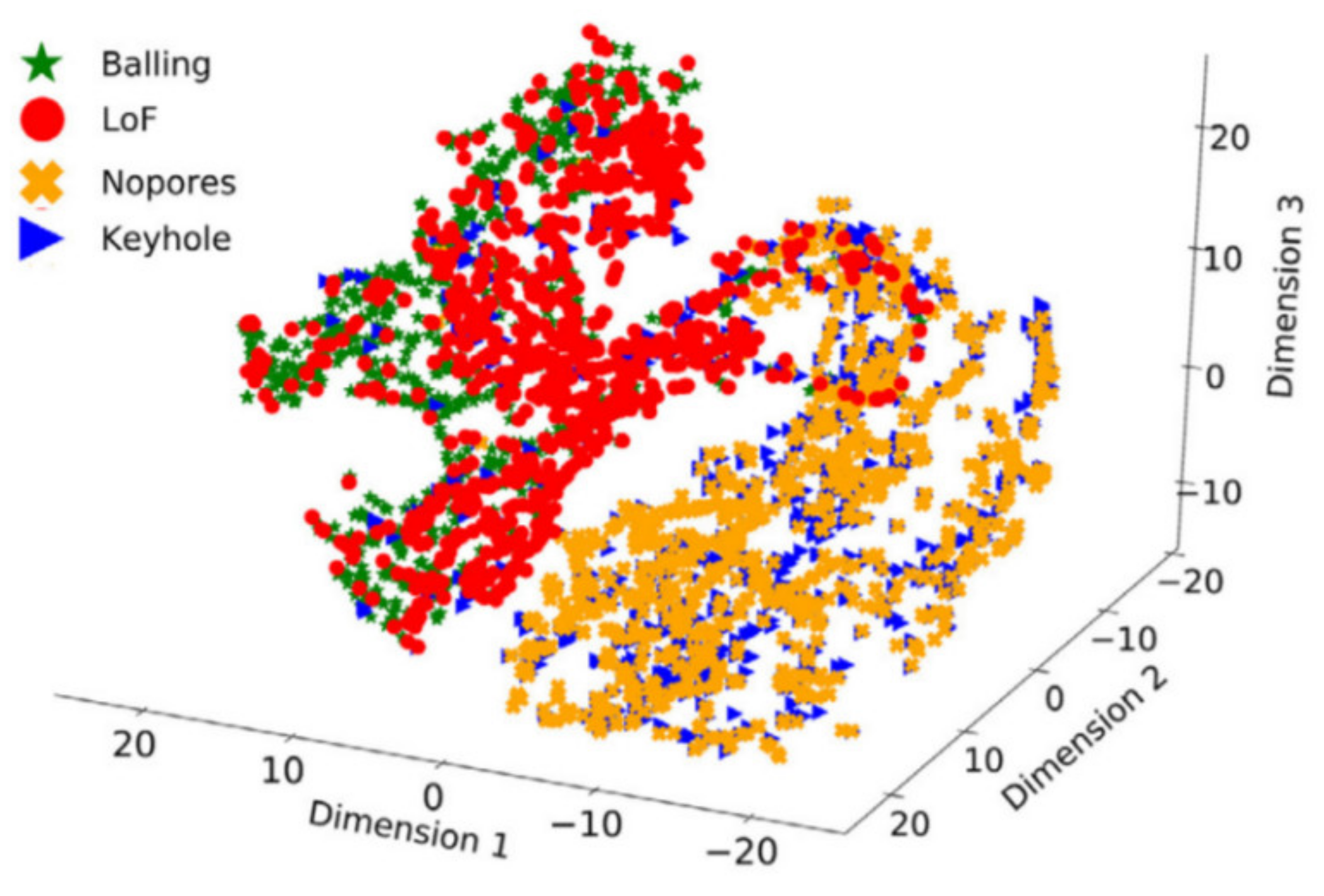
| PAC AM4I | Sidewalls of the build chamber | 316L | tracks | Scan speed | Time Frequency Time–Frequency | PCA t-SNE (unsupervised) | NA | Clustering the AE signals from different laser melting conditions balling lack of fusion, no pores, and keyholes. | [108] |
| PCB microphone | Sidewalls of the build chamber | 316L | tracks | Scan speed | Time Frequency Frequency denoised | DBN MLP SVM (supervised) | 70–95 46–82 67–98 | Comparing between different ML algorithms in different AE signals domains. | [118] |
| Fiber Bragg grating | Sidewalls of the build chamber | 316L | cuboid 10 × 10 × 20 | Scan speed | Time–Frequency | SCNN (supervised) | 83–89 | laser scanning velocity has an impact on the self-extraction of the distinct features in the SCNN. | [120] |
| Fiber Bragg grating | Sidewalls of the build chamber | 316L | cuboid 10 × 10 × 20 | Scan speed | Time–Frequency | SCNN CNN Xception ResNet (supervised) | 78–91 53–63 54–68 60–75 | SCNN has better classification and faster time than other ML algorithms used. | [122] |
| Fiber Bragg grating | Sidewalls of the build chamber | 316L | cuboid 10 × 10 × 20 | Scan speed | Time–Frequency | CNN (supervised) | 79–84 | Ability to classify different quality levels. | [119] |
| Fiber Bragg grating | Sidewalls of the build chamber | 316L | 1 cube 10 × 10 × 20 | Scan speed | Time–Frequency | CNN (RL-based) | 74–82 | taking advantage of the outstanding RL self-learning capabilities in future systems may reduce the costs for preparing the training datasets. | [114] |
| Piezoceramic sensor | In build plate | 316L | 54 cubes (5 × 5 x 5) | Laser power Scan speed | Time–Frequency | ANN (supervised) | 76–86 55–88 | Classifying different quality levels and different parts complexity. | [79] |
| WSα | In build plate | 316L | Cylinders 10 mm diameter 10 mm height | Laser power | Frequency denoised | DBN (supervised) K-means, (unsupervised) | 70–91 | Classifying different density levels. | [121] |
| WSα | In build plate | H13 | Cylinders 10 mm diameter 10 mm height | Laser power | Frequency denoised | DBN(Supervised) PCA/GMM (unsupervised) Hierarchical K-Means (unsupervised) VAE (supervised) | 93–70 | Classifying different density levels. Model generalization. | [74] |
| Camera Location | Specifications | Material | Part Geometry | ML Algorithm | Accuracy % | Objective | Ref. |
|---|---|---|---|---|---|---|---|
| Off-axis above build chamber | 1.3 megapixel 290 μm/pixel | Ti6Al4V AlSi10Mg Inconel 718 316L 17-4 Bronze alloy | Hamerschlag model case study | BoW (unsupervised) | 50–91 | Classify six types of powder bed anomalies: recoater hopping, recoater streaking, debris, superelevations, part failure, and incomplete spreading. | [123] |
| Off-axis inside build chamber | 16–65 μm/pixel | Ti6AL4V | Cylinders 25 mm length 10 mm diameter | SVM Tree LDA K-NN Ensemble FF-NN (supervised) | 89 79 82 78 85 84 | Quantify the count of pores as process parameters, change and monitor the process parameters that might cause more porosity. | [124] |
| Off-axis Inside build chamber | 36.3-megapixel | GP-1 | Stepped cylinder | SVM (supervised) | 85 | Detect part discontinuities by using in situ images. | [85] |
| Off-axis Inside chamber | 8.8 megapixel 4096 × 2160 pixel | Inconel 625 | Cube samples with 80 mm side | BC (supervised) PCA | 89 | Classify different meltpool conditions influenced by the formation of pores and cracks in printed parts. | [126] |
| Off-axis Inside build chamber | 36.3-megapixel | Ti6AL4V | Cylindrical coupons | NN CNN (supervised) | 86 | Defect detection from layerwise images and comparing CNN to NN. | [125] |
| Off-axis Inside build chamber | 36.3 megapixel 7360 × 4912 pixels | Ti6Al4V | Drag link joint | DCNN (supervised) | 92 | Detect flaws in geometry compared to CAD from layerwise imaging. | [127] |
| Off-axis Inside build chamber | 36.3 megapixel 7360 × 4912 pixels | Ti6Al4V | Thin-walled feature | DCNN (supervised) | 85–98 | Predict process defects in thin walls. | [128] |
| Off-axis Outside build chamber | 24.2 megapixel | Inconel 718 | Disc 20 mm height 40 mm diameter | DCNN (supervised) | 99 | Classify parts printed at different VED levels standard, low, high, and very low. | [129] |
| Camera Location | Specifications | Material | Part Geometry | ML Algorithm | Accuracy % | Objective | Ref |
|---|---|---|---|---|---|---|---|
| Off-axis Outside chamber/above | 6.35 mm × 6.35 mm 6.2 µm/pixel 6400 fps | Inconel | Laser tracks (supported and unsupported) | BoW (unsupervised) | NA | Detect keyholing porosity and balling instability. | [101] |
| Off-axis outside chamber | 250 µm/pixel 1000 fps | Maraging Steel | Parallelepiped 5 × 5 × 12 | LR (supervised) | NA | Investigate the appropriateness of including spatter information to characterize the process quality. | [86] |
| Off-axis outside chamber | 12 × 5 mm 2000 fps | 316L | Melt tracks | PCA–SVM CNN (supervised) | 90 92 | Identify different quality levels of parts printed at different process parameters. | [130] |
| Coaxial Outside chamber/above | 14 µm/pixel 256 × 256 mm 1 kHz frame rate 12–50 frames | 316L | 5 mm laser tracks | CNN (supervised) | 93 | Measure the mean and standard deviation of track width and classify the continuity of the track. | [131] |
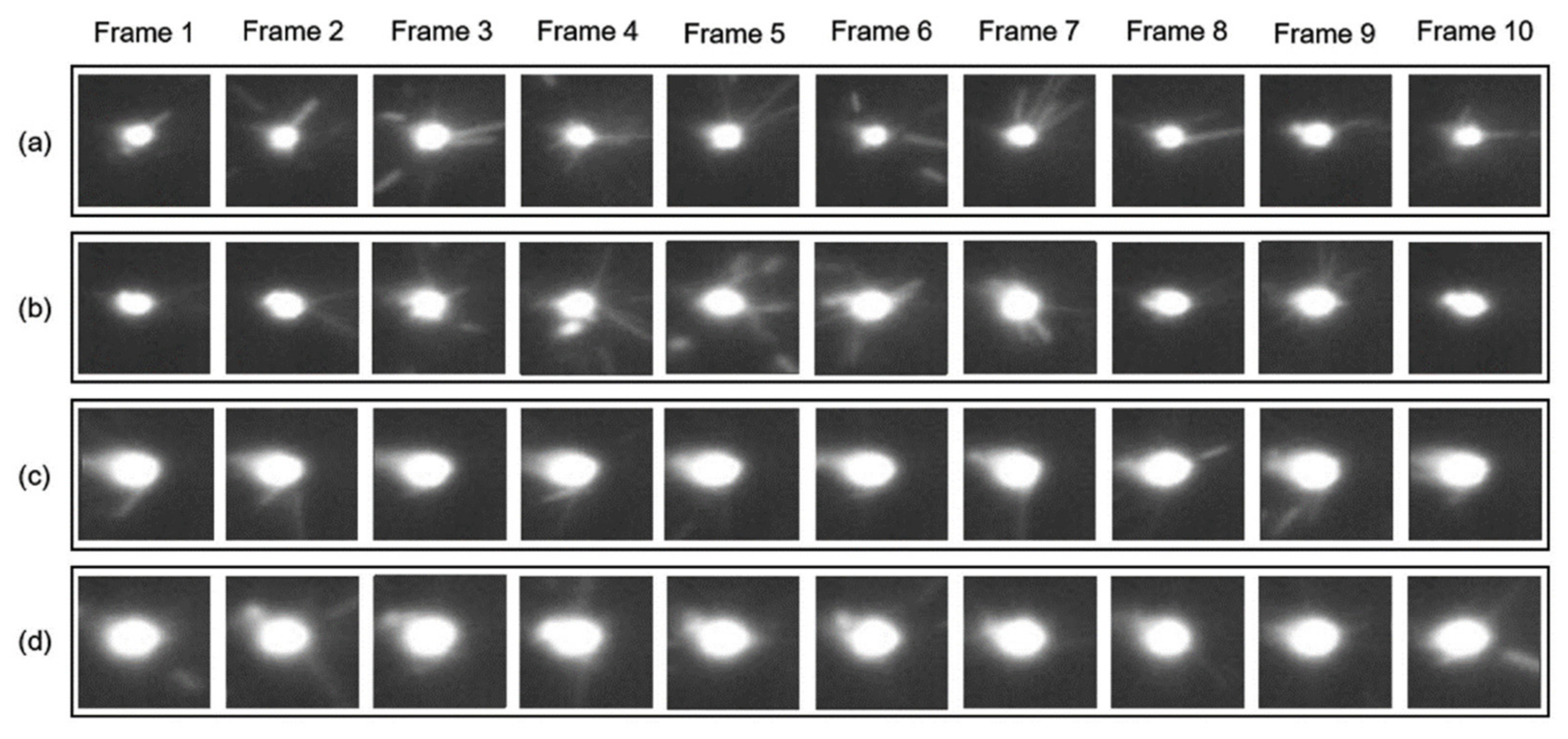
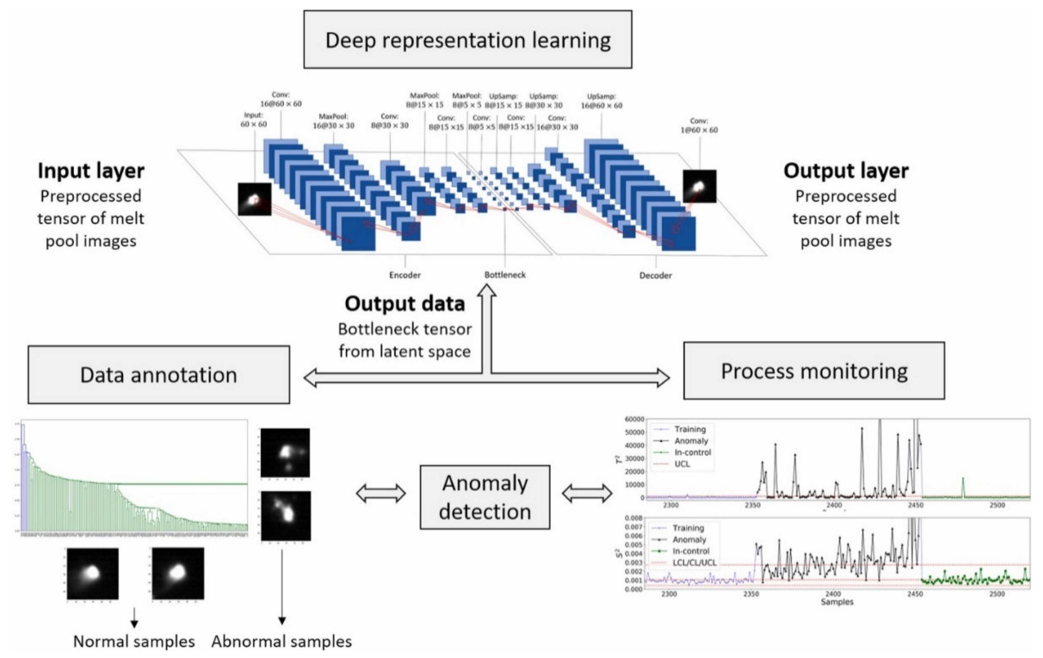
| Coaxial Outside chamber/above | 128 × 120 mm 2.5 kHz | Inconel 625 | Cube specimen 810 × 10 × 5 | NBEM DL–CAE (supervised) | 89 95 | Learn a low-dimensional but deep representation from meltpool data for anomaly detection. | [132] |
| Off-axis Outside chamber/side | 1 Megapixel 1024 × 1024 pixels 5000 fps | 304 L | Laser tracks | DBN CNN MLP (supervised) | 83 82 70 | Recognition of melt state and optimize process parameters to decrease part quality. | [83] |
| Coaxial Outside chamber/above | 1.3 M 512 × 512 mm 2.5 kHz | 316L | Cube specimen 8.5 × 8.5 × 4 | DBN PCA (supervised) | NA | Classify and predict the accuracy depending on image intensity. | [82] |
| Sensor Type | Sensor Location | Specifications | Material | Signature | Part | ML Algorithm | Accuracy % | Objective | Ref. |
|---|---|---|---|---|---|---|---|---|---|
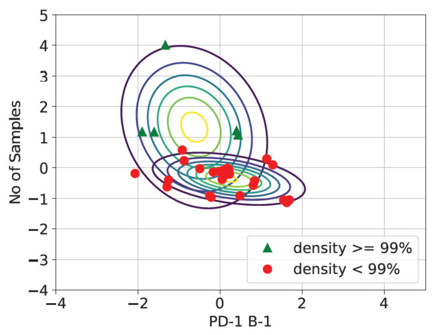
| 3 Photodiodes | Coaxial | Wavelength 700 to 1050 nm - sensitive to plasma emissions Wavelength 1080 to 1700 nm - sensitive to thermal radiation suitable to measure laser beam intensity | N/A | Meltpool temperature | Cubes | SVD K-means GMM GPR (semi-supervised) | 93% | Density classification | [133] |
| Pyrometer | Coaxial | N/A | 316L | Meltpool temperature | Cubes | SVM MLP 1D CNN (supervised) | 90% 91% 81% | Density prediction | [134] |
| 2 Pyrometers | Off-axis | Heat emission light in the range of 1500 to 1700 nm 100 Hz. | 316L | Scanned layer temperature | Cubes | K-NN (supervised) | 92–94% | Pore detection | [100] |
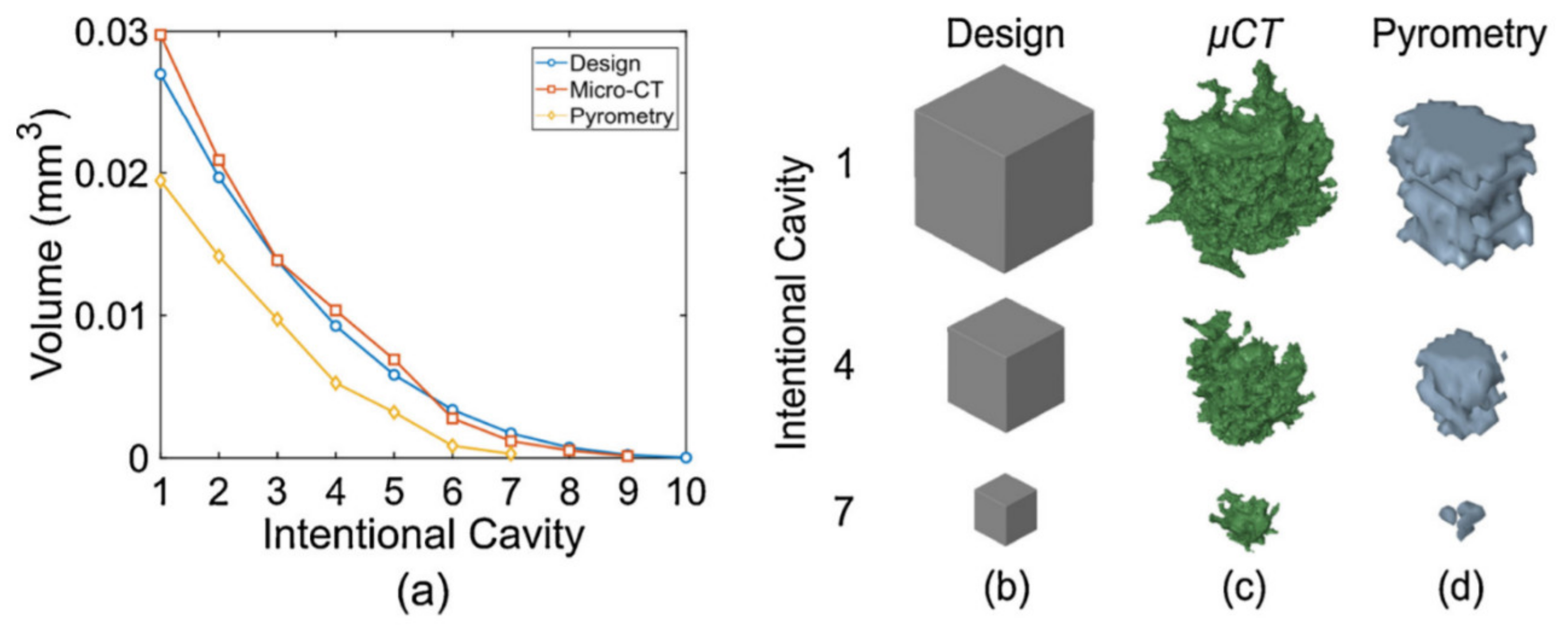
| Two wavelength Pyrometer | Off-axis | Field of view: 1300 × 1000, frame rate 100 Hz field of view: 600 × 50, frame rate 2.8 kHz 30 × 27 mm 2 area, spatial resolution of 24 μm per pixel. used frame rate of 250 Hz | 17–4 precipitation hardened SS | Meltpool temperature | 5.5 × 8 × 9 prism with intentional cavity | LR SVM KNN RF (supervised) | 96% | Cavity detection | [137] |
| Two wavelength Pyrometer | Off-axis | FOV 65 × 80 pixels Resolution of 21 μm/pixel 90 μs exposure Sampling rate 6–7 kHz | 316L | Meltpool temperature | L shape With intentional defects | k-d tree (supervised) | NA | Pore detection | [138] |
| Infrared camera | Off-axis Above the build chamber | Optical resolution 640 × 480 sensor elements spectral range from 4.8 to 5.2 µm. 50 images per second spatial resolution 1289 × 768 pixel | H13 | Scanned layer temperature | Cubes | CNN (supervised) | 97% | Delamination and spatter detection | [105] |
| Infrared camera | N/A | 856 × 658 spatial resolutions, 12-bit analog to digital converter (ADC), 30 Hz frame rate, wavelengths 750–950 µm. | N/A | Scanned layer temperature | Part with geometric grooves | CNN (supervised) | 60% | Detect geometry | [139] |
| Infrared Camera | Off-axis | 192 × 100 pixel 10,000 Hz 30 µm pixel size | Ti6Al4V | Meltpool temperature | Laser tracks | LR RFC GBC GPC (supervised) | 88% 87% 89% 84% | Predict the probability of porosity formation. | [67] |
| Machine Learning Technique | Process | Control Strategy | Data | Reference |
|---|---|---|---|---|
| Sequential decision making through the Markov decision process framework | L-PBF | Optimal control | Imaging | Yao et al. [154] |
| CNN | FDM | Adjustment of filaments flow rate | Imaging | Jin et al. [155] |
| Radial basis function networks (RBF) | L-PBF | Feedforward control | Temperature using pyrometer | Reiff et al. [21] |
| Support vector machine (SVM) | FDM | PID control | Imaging | Liu et al. [157] |
| Reinforcement learning (RL) | L-PBF | Corrective actions to prevent the onset of defects | Acoustic emissions | Marinelli et al. [158] |
Publisher’s Note: MDPI stays neutral with regard to jurisdictional claims in published maps and institutional affiliations. |
© 2021 by the authors. Licensee MDPI, Basel, Switzerland. This article is an open access article distributed under the terms and conditions of the Creative Commons Attribution (CC BY) license (https://creativecommons.org/licenses/by/4.0/).
Share and Cite
Mahmoud, D.; Magolon, M.; Boer, J.; Elbestawi, M.A.; Mohammadi, M.G. Applications of Machine Learning in Process Monitoring and Controls of L-PBF Additive Manufacturing: A Review. Appl. Sci. 2021, 11, 11910. https://doi.org/10.3390/app112411910
Mahmoud D, Magolon M, Boer J, Elbestawi MA, Mohammadi MG. Applications of Machine Learning in Process Monitoring and Controls of L-PBF Additive Manufacturing: A Review. Applied Sciences. 2021; 11(24):11910. https://doi.org/10.3390/app112411910
Chicago/Turabian StyleMahmoud, Dalia, Marcin Magolon, Jan Boer, M. A. Elbestawi, and Mohammad Ghayoomi Mohammadi. 2021. "Applications of Machine Learning in Process Monitoring and Controls of L-PBF Additive Manufacturing: A Review" Applied Sciences 11, no. 24: 11910. https://doi.org/10.3390/app112411910