Article

The Study of Generalized Synchronization between Two Identical Neurons Based on the Laplace Transform Method

School of Environment and Architecture, University of Shanghai for Science and Technology, Shanghai 200093, China
*
Author to whom correspondence should be addressed.
Appl. Sci. 2021, 11(24), 11774; https://doi.org/10.3390/app112411774
Submission received: 10 November 2021 / Revised: 1 December 2021 / Accepted: 6 December 2021 / Published: 11 December 2021
(This article belongs to the Topic Dynamical Systems: Theory and Applications)

Abstract

:
In this paper, a new method is proposed based on the auxiliary system approach to investigate generalized synchronization between two identical neurons with unidirectional coupling. Different from other studies, the synchronization error system between the response and auxiliary systems is converted into a set of Volterra integral equations according to the Laplace transform method and convolution theorem. By using the successive approximation method in the theory of integral equations, an analytical criterion for the detection of generalized synchronization between two identical neurons is obtained. It is found that there is a time difference between two signals of neurons when the generalized synchronization between them is achieved. Furthermore, the value of the time difference has no relation to the generalized synchronization condition but depends on the coupling function between two neurons. The study in this paper shows that one can construct a coupling function between two identical neurons using the current signal of the drive system to predict its future signal or make its past signal reappear.

1. Introduction

Over the past few decades, chaos synchronization has received a lot of interest and attention because it plays an important role in understanding the feature of coupled chaotic oscillators [1]. Generally speaking, when one chaotic system (drive system) sends a signal to the other system (response system), their chaotic trajectories may remain in step with each other under some conditions. Many types of synchronization have been revealed in dynamical systems, such as complete synchronization (CS), lag synchronization (LS), anticipated synchronization (AS), generalized synchronization (GS), and so on [2,3,4]. If the state variables of the drive and response systems become synchronized with a time difference τ , then τ = 0 means that CS between the drive and response systems is reached; τ > 0 and τ < 0 indicate that LS and AS are achieved, respectively. GS is considered to be the chaos synchronization most frequently occurring in natural systems [5,6,7], which is an extension of CS, LS, and AS. GS is usually defined in the frame of drive–response systems with nonidentical dynamics, characterized by the existence of a functional relation between the state variables of the drive and response systems. Different types of synchronization (such as CS, LS, AS, etc.) can be viewed as special cases of GS depending on the choice of functional relations. Thus, GS is more intricate due to the complex functional relation between the state variables of the drive and response systems.
One of most exciting problems to GS is how to analytically detect the existence of a functional relation between the signals of the drive and response systems. Kocarev and Parlitz [6] pointed out that GS only appears when the response system is stable asymptotically. Then one can investigate GS detection by using the response Lyapunov exponents method or Lyapunov function approach [8,9,10]. The Lyapunov function technology is one of the earliest methods to analytically establish the synchronization condition in coupled oscillators. However, how to find an appropriate Lyapunov function is the key to using this method. In addition, the synchronization condition obtained by using the Lyapunov function method is usually sufficient and highly conserved. Abarbanel et al. [11] proposed an indirect way of analytically verifying GS between two chaotic systems with unidirectional coupling by constructing an identical copy of the response system called the auxiliary system, which is driven by the same driving signal. The auxiliary system approach proved that GS between the drive–response system will be achieved if CS between the response and auxiliary systems occurs with different initial conditions. The master stability function method [12] was recommended in the auxiliary system approach to obtain the conditions for CS between the response and auxiliary system, whereas the auxiliary system approach can only be implemented numerically in most cases. It is a very meaningful topic to develop more convenient and effective approaches to analytically detect GS in a drive–response system.
In recent years, the dynamical behavior of neurons has received increasing interest due to its applications in brain science, medical technology, artificial intelligence, and so on. Synchronization in neural systems in the brain is considered to be a crucial phenomenon related to cognition and the correlation of behavior [13,14,15,16] because nerve cells do not have intelligence of their own. It is feasible to understand information processing in the brain by investigating synchronization between neurons [17,18,19,20,21,22]. The Hodgkin–Huxley (HH) Equation [23] was usually used to construct neural systems and exhibit the neural dynamic behavior. A simplified version of the HH equation, such as the FitzHugh–Nagumo (FHN) model [24] and the Hindmarsh–Rose (HR) model [21,25,26,27], which can show excitability and neural bursting of a neuron, is more convenient in the investigation of neural behavior based on nonlinear dynamical theory. The study of synchronization in FHN and HR neurons makes plenty of sense in understanding their information transfer process.
In this paper, GS between two identical FHN and HR neurons with unidirectional coupling is investigated based on the auxiliary system approach. Different from other studies, the synchronization error between the response and auxiliary systems is found to satisfy a Volterra integral equation from the Laplace transform method and convolution theorem. According to the successive approximation method [28] in the Volterra integral equation theory, an analytical criterion is given for the detection of GS between two identical FHN and HR neurons. It is found that there is a time difference τ between the signals of the drive and response systems when the GS condition obtained by the analytical criterion given in this paper is satisfied. Moreover, the GS condition has no relation to the value of τ . Numerical simulations for FHN and HR neural systems are carried out to verify correctness of the analytical results. From Taylor’s expansion of the functional relation of GS, our results show that it is feasible to predict future signals or make a past signal reappear of a neuron by using its current signal.
The rest of the paper is organized as follows: In Section 2, the GS between two identical FHN neurons with unidirectional coupling is studied using the Laplace transform method. In Section 3, the functional relation of GS between two FHN neurons is discussed, and numerical simulations are carried out to verify the correctness of the theoretical results. In Section 4, the GS between two identical HR neurons is investigated to show that the analytical results for FHN neurons is the same for a chaotic case. The conclusions are drawn in Section 5.

2. GS between Two FHN Neurons

2.1. GS in Unidirectionally Coupled FHN Neurons

A single FHN neuron is given in the following form
v ˙ = v v 3 / 3 w + I e x t , w ˙ = γ ( v + a b w ) ,
where v and w represent the potential difference and a recovery current variable, respectively. a , b , and γ are positive parameters, and 0 < b < 1 , 0 < γ 1 . I e x t is the external current input. Assume that ( v 0 , w 0 ) is the equilibrium point of System (1), that is,
v 0 v 0 3 / 3 w 0 + I e x t = 0 , v 0 + a b w 0 = 0 .
For convenience, move equilibrium ( v 0 , w 0 ) to the origin in System (1). Substituting u 1 = v v 0 , u 2 = w w 0 into System (1), one has
u ˙ 1 = u 1 3 / 3 + c u 1 2 + d u 1 u 2 , u ˙ 2 = γ ( u 1 b u 2 ) ,
where c = v 0 , d = 1 v 0 2 , v 0 is the unique real root to equation v 0 3 3 + ( 1 1 b ) v 0 a b + I e x t = 0 .
The behavior of two unidirectionally coupled FHN neurons is considered
u ˙ 1 = u 1 3 / 3 + c u 1 2 + d u 1 u 2 , u ˙ 2 = γ ( u 1 b u 2 ) , u ˙ 3 = u 3 3 / 3 + c u 3 2 + d u 3 u 4 + k ( u 3 H ( u 1 ) ) , u ˙ 4 = γ ( u 3 b u 4 ) ,
in which k is the coupling strength, H ( u 1 ) is a continue function of u 1 . The first and second neurons in Equation (3) are referred to as a drive and response, respectively. In this paper, we consider that System (3) possesses the following property
lim t | | u 3 H ( u 1 ) | | = 0 .
In fact, it can be said that there exists the property of GS in System (3) with a transformation H between u 1 and u 3 .

2.2. Necessary Conditions for GS between Two FHN Neurons

Based on the auxiliary system approach [11], the auxiliary system corresponding to System (3) is given by
u ˙ 5 = u 5 3 / 3 + c u 5 2 + d u 5 u 6 + k ( u 5 H ( u 1 ) ) , u ˙ 6 = γ ( u 5 b u 6 ) .
Then Condition (4) will lead to
lim t | | u 3 u 5 | | = 0 .
By defining
e 1 = u 3 u 5 2 , e 2 = u 3 + u 5 2 ,
Systems (3) and (5) become
u ˙ 1 = u 1 3 / 3 + c u 1 2 + d u 1 u 2 , u ˙ 2 = γ ( u 1 b u 2 ) , u ˙ 4 = γ ( e 1 + e 2 b u 4 ) , u ˙ 6 = γ ( e 2 e 1 b u 6 ) , e ˙ 1 = e 1 3 / 3 + ( e 2 2 + 2 c e 2 + d + k ) e 1 u 4 u 6 2 , e ˙ 2 = e 2 3 / 3 + c ( e 1 2 + e 2 2 ) + ( d + k e 1 2 ) e 2 u 4 + u 6 2 k H ( u 1 ) .
Condition (6) is equivalent to
lim t | | e 1 | | = 0 .
GS in System (3) appears if Condition (9) is satisfied. Consider the Laplace transform defined as follows:
u ^ i ( s ) = L [ u i ] ( s ) = 0 + u i ( t ) e s t d t , u i ( t ) = L 1 [ u ^ i ] ( t ) = 1 2 π i σ i σ + i u ^ i ( s ) e s t d s , i = 1 , 2 , 4 , 6 , e ^ j ( s ) = L [ e j ] ( s ) = 0 + e j ( t ) e s t d t , e j ( t ) = L 1 [ e ^ j ] ( t ) = 1 2 π i σ i σ + i e ^ j ( s ) e s t d s , j = 1 , 2 .
By taking the Laplace transform on both sides of equations in Equation (8), one has
( s d ) u ^ 1 + u ^ 2 = u 10 + W ^ 1 , ( s + b γ ) u ^ 2 = u 20 + γ u ^ 1 , ( s + b γ ) u ^ 4 = u 40 + γ ( e ^ 1 + e ^ 2 ) , ( s + b γ ) u ^ 6 = u 60 + γ ( e ^ 2 e ^ 1 ) , ( s d k ) e ^ 1 + 1 2 ( u ^ 4 u ^ 6 ) = e 10 + W ^ 2 , ( s d k ) e ^ 2 + 1 2 ( u ^ 4 + u ^ 6 ) = e 20 + W ^ 3 ,
where u i 0 , i = 1 , 2 , 4 , 6 , and e j 0 , j = 1 , 2 , are given initial values of System (8), and W ^ k , k = 1 , 2 , 3 are the Laplace transform of the nonlinear parts in the first, fifth, and last equations in Equation (8), respectively
W ^ 1 = 0 + [ u 1 3 / 3 + c u 1 2 ] e s t d t 0 + W 1 e s t d t , W ^ 2 = 0 + [ e 1 2 / 3 e 2 2 + 2 c e 2 ] e 1 e s t d t 0 + W 2 e s t d t , W ^ 3 = 0 + [ e 2 3 / 3 e 1 2 e 2 + c ( e 1 2 + e 2 2 ) k H ( u 1 ) ] e s t d t 0 + W 3 e s t d t .
Substituting the third and fourth equations into the fifth equation in Equation (11) yields
e ^ 1 = ( s + β 3 ) e 10 + β 4 s 2 + β 1 s + β 2 + ( s + β 3 ) W ^ 2 s 2 + β 1 s + β 2 .
where β 1 = b γ d k , β 2 = [ 1 ( k + d ) b ] γ , β 3 = b γ , β 4 = ( u 60 u 40 ) / 2 . To analyze whether | | e 1 | | 0 holds when t , taking the inverse Laplace transform on both sides of Equation (12), produces
e 1 = e 10 Ψ 1 ( t ) + β 4 Ψ 2 ( t ) + 0 t Ψ 1 ( t ξ ) W 2 d ξ , = e 10 Ψ 1 ( t ) + β 4 Ψ 2 ( t ) + 0 t Ψ 1 ( t ξ ) [ e 1 ( ξ ) 2 / 3 e 2 ( ξ ) 2 + 2 c e 2 ( ξ ) ] e 1 ( ξ ) d ξ ,
where Ψ 1 , 2 ( t ) represent the inverse Laplace transform defined in Equation (10):
Ψ 1 ( t ) = L 1 [ s + β 3 s 2 + β 1 s + β 2 ] = e β 1 t / 2 [ cosh ( ϕ 1 t ) + 2 β 3 β 1 2 ϕ 1 sinh ( ϕ 1 t ) ] , β 1 0 e β 1 t / 2 [ 1 + 2 ( 2 β 3 β 1 ) t ] , β 1 = 0 Ψ 2 ( t ) = L 1 [ 1 s 2 + β 1 s + β 2 ] = sinh ( ϕ 1 t ) ϕ 1 e β 1 t / 2 , β 1 0 t e β 1 t / 2 , β 1 = 0
in which ϕ 1 = β 1 2 4 β 2 / 2 .
Obviously, from Equation (13), the necessary condition for | | e 1 | | 0 is Ψ 1 , 2 0 when t . Then, β 1 / 2 ± R e { ϕ 1 } < 0 , in which R e { ϕ 1 } represents the real part of ϕ 1 , should be satisfied from Equation (14). Actually, this means that the two roots of equation s 2 + β 1 s + β 2 = 0 have negative real parts. From the Routh–Hurwitz criterion, the following condition is necessary and sufficient to guarantee β 1 / 2 ± R e { ϕ 1 } < 0
β 1 > 0 , β 2 > 0 .
Under Condition (15), Equation (13) becomes
e 1 = 0 t Ψ 1 ( t ξ ) [ e 1 ( ξ ) 2 / 3 e 2 ( ξ ) 2 + 2 c e 2 ( ξ ) ] e 1 ( ξ ) d ξ .

2.3. Sufficient Conditions for GS in System (3)

Equation (16) is a Volterra integral equation that can be solved using the successive approximation method [28]. For the sake of clarity, the main results given by J.A. Nohel [28] are introduced briefly first. For the following system of integral equations of the form
y ( t ) = ϕ ( t ) + 0 t f ( t τ ) g ( τ , y ( τ ) ) d τ ,
where f is a n by n matrix, and ϕ and g are given vectors with n components. Additionally, the following conditions are satisfied
(1)
| y | < ;
(2)
For 0 t < t 0 ( 0 < t 0 < + ), ϕ and g are continuous;
(3)
For any 0 < ϵ < t 0 , | f | L [ 0 , ϵ ] .
Theorem 1
(Local existence). Equation (17) has at least one continuous solution on 0 t < t 0 . Furthermore, the solution is unique if for any η > 0 , there exists a constant ψ ( η ) > 0 such that
| g ( t , y 1 ) g ( t , y 2 ) | ψ ( η ) | y 1 y 2 | , ( | y 1 | , | y 2 | η ) .
Theorem 2.
If conditions in Theorem 1 hold, then the successive approximations
Ω 0 ( t ) = 0 , Ω n + 1 ( t ) = ϕ ( t ) + 0 t f ( t τ ) g ( τ , Ω n ( τ ) ) d τ , n = 0 , 1 , 2 ,
uniformly converge to the unique continuous solution y ( t ) = Ω ( t ) of Equation (17) on [ 0 , t ] .
Comparing Equations (16) and (17), one has
y ( t ) = e 1 ( t ) , ϕ ( t ) = 0 , f ( t ) = Ψ 1 ( t ) , g ( t , y ( t ) ) = [ e 1 ( t ) 2 / 3 e 2 ( t ) 2 + 2 c e 2 ( t ) ] e 1 ( t ) .
g ( t , y ( t ) ) in Equation (20) is smooth enough to satisfy Condition (18). Equation (16) has a unique solution according to Theorem 1, which can be obtained by substituting Equation (20) into Equation (19). From the successive approximations, e 1 ( t ) = 0 is the unique solution to Equation (16). Therefore, Condition (15) is sufficient for e 1 ( t ) = 0 .

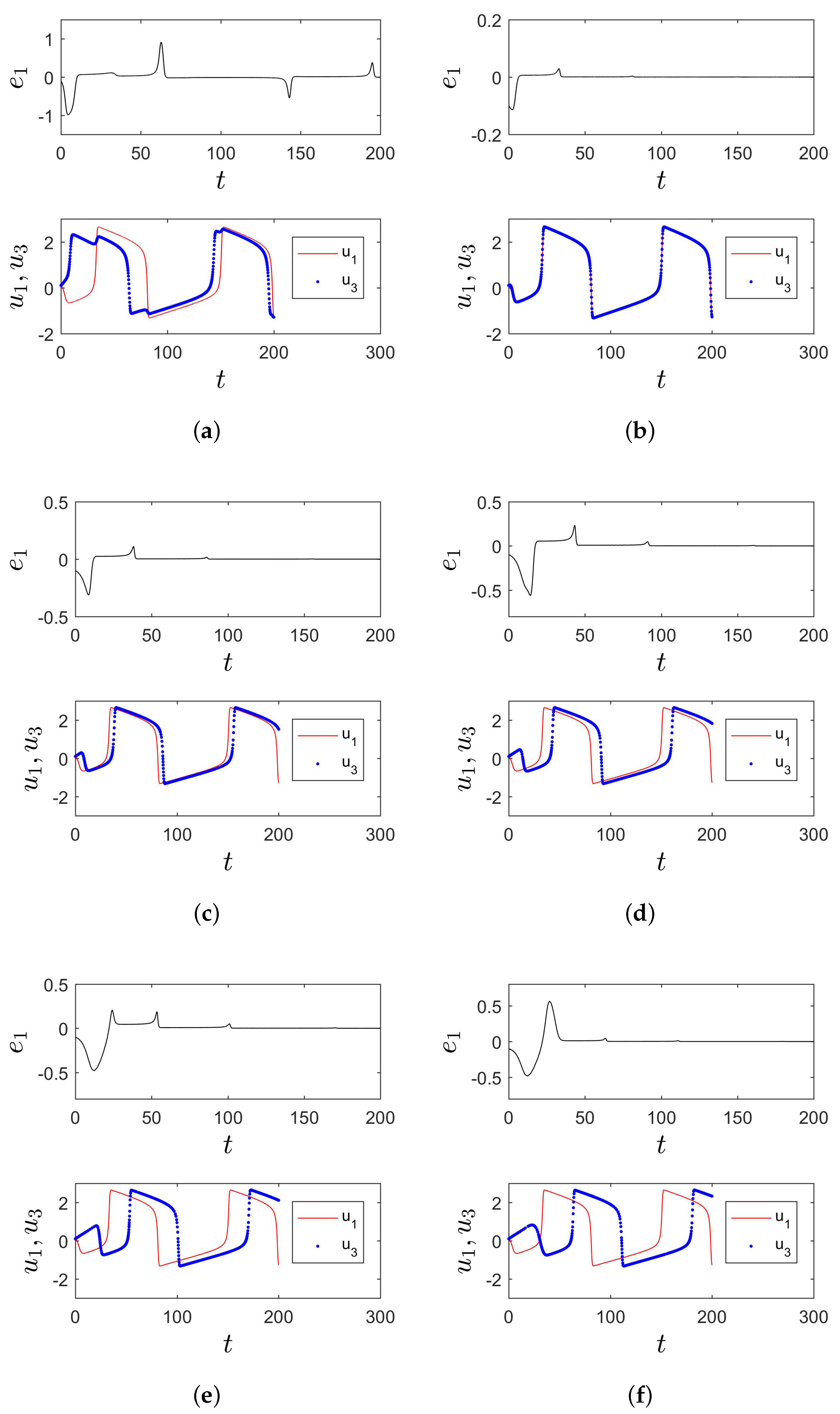
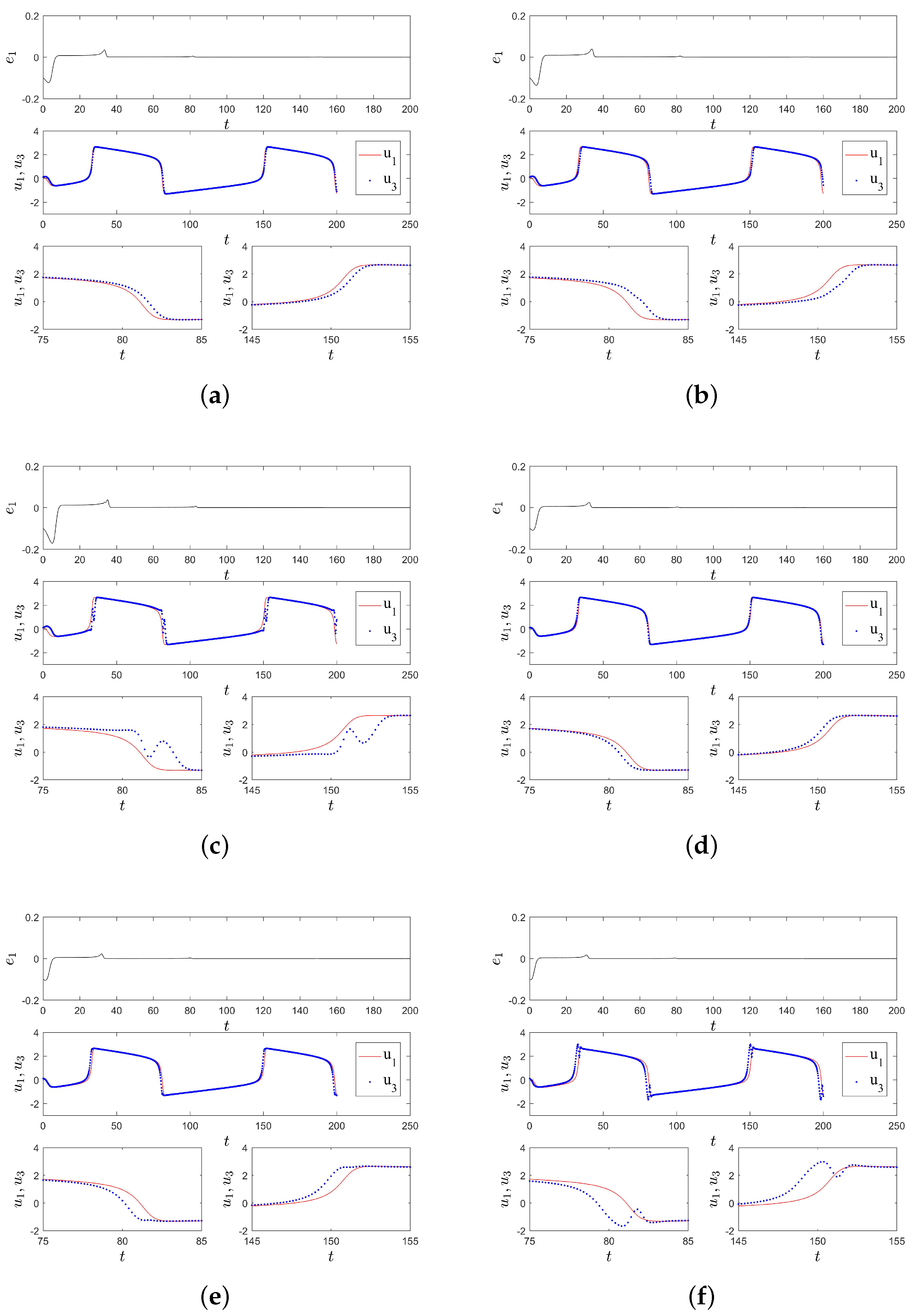
3. Analysis for GS between Two FHN Neurons and Numerical Simulations

For clarity, denote System (3) by [ U ˙ 1 , U ˙ 2 ] T = [ F ( U 1 ) , F ( U 2 ) ] T + k [ 0 , U 2 H ( U 1 ) ] T , where U 1 = [ u 1 , u 2 ] T and U 2 = [ u 3 , u 4 ] T . The following equation is necessary for the appearance of G S in System (3) with the functional relation U 2 = H ( U 1 ) :
D H ( U 1 ) · F ( U 1 ) = F ( H ( U 1 ) ) + k [ U 2 H ( U 1 ) ] .
Clearly, H ( U 1 ) = U 1 ( t τ ) , τ 0 , should be satisfied for the occurrence of GS in System (3). Consider a = 0.7 , b = 0.8 , γ = 0.02 , I e x t = 0.6 , and H ( u 1 ) = u 1 ( t τ ) in System (3). From Equation (15), the condition for occurrence of GS in System (3) can be given by
k < b γ d = 0.521 a n d k < 1 b d b = 0.713 .
Therefore, the GS condition that H ( u 1 ) = u 1 ( t τ ) in System (3) is k < 0.521 . It is worth mentioning that the GS condition has no relation to the value of τ . Synchronization error u 3 u 5 and functional relation between u 1 and u 3 are depicted in Figure 1 for different values of k and τ , in which the initial conditions of drive, response, and auxiliary systems are chosen as u 1 ( t ) = 0.1 , t ( τ , 0 ] , u 2 ( 0 ) = 0.1 , ( u 3 ( 0 ) , u 4 ( 0 ) ) = ( 0.1 , 0.02 ) , and ( u 5 ( 0 ) , u 6 ( 0 ) ) = ( 0.3 , 0.02 ) , respectively. Figure 1 shows that the functional relation H ( u 1 ) = u 1 ( t τ ) between two FHN neurons is achieved when k < 0.521 for any value of τ .
Near τ = 0 , H ( u 1 ) = u 1 ( t τ ) can be approximately expanded as
H ( u 1 ) = u 1 ( t τ ) = u 1 ( t ) d u 1 d t τ + 1 2 ! d 2 u 1 d t 2 τ 2 1 3 ! d 3 u 1 d t 3 τ 3 + O ( τ 3 ) ,
where O ( τ 3 ) represents the higher order terms of τ greater than 3. From System (3), one has
d u 1 d t = u 1 3 / 3 + c u 1 2 + d u 1 u 2 , d 2 u 1 d t 2 = ( u 1 2 + 2 c u 1 + d ) d u 1 d t γ ( u 1 b u 2 ) , d 3 u 1 d t 3 = ( u 1 2 + 2 c u 1 + d ) d 2 u 1 d t 2 + 2 ( c u 1 ) ( d u 1 d t ) 2 γ d u 1 d t + b γ 2 ( u 1 b u 2 ) .
Consider
H ( u 1 ) = u 1 ( t ) d u 1 d t τ + 1 2 ! d 2 u 1 d t 2 τ 2 1 3 ! d 3 u 1 d t 3 τ 3 G ( u 1 , u 2 , τ ) ,
in System (3). As shown in Figure 2a,b,d,e, the functional relation u 3 = u 1 ( t τ ) is approximately reached between two FHN neurons in System (3) with H ( u 1 ) = G ( u 1 , u 2 , τ ) for a small value of τ when k = 0.7 . However, with increase in τ , the functional relation is destroyed (Figure 2c,f). More higher order terms of τ need to be added in G ( u 1 , u 2 , τ ) to decrease the error between u 1 ( t τ ) and u 3 . This means that one can design a coupling function between two identical FHN neurons using the current signal of the drive system to predict its future signal or make its past signal reappear.

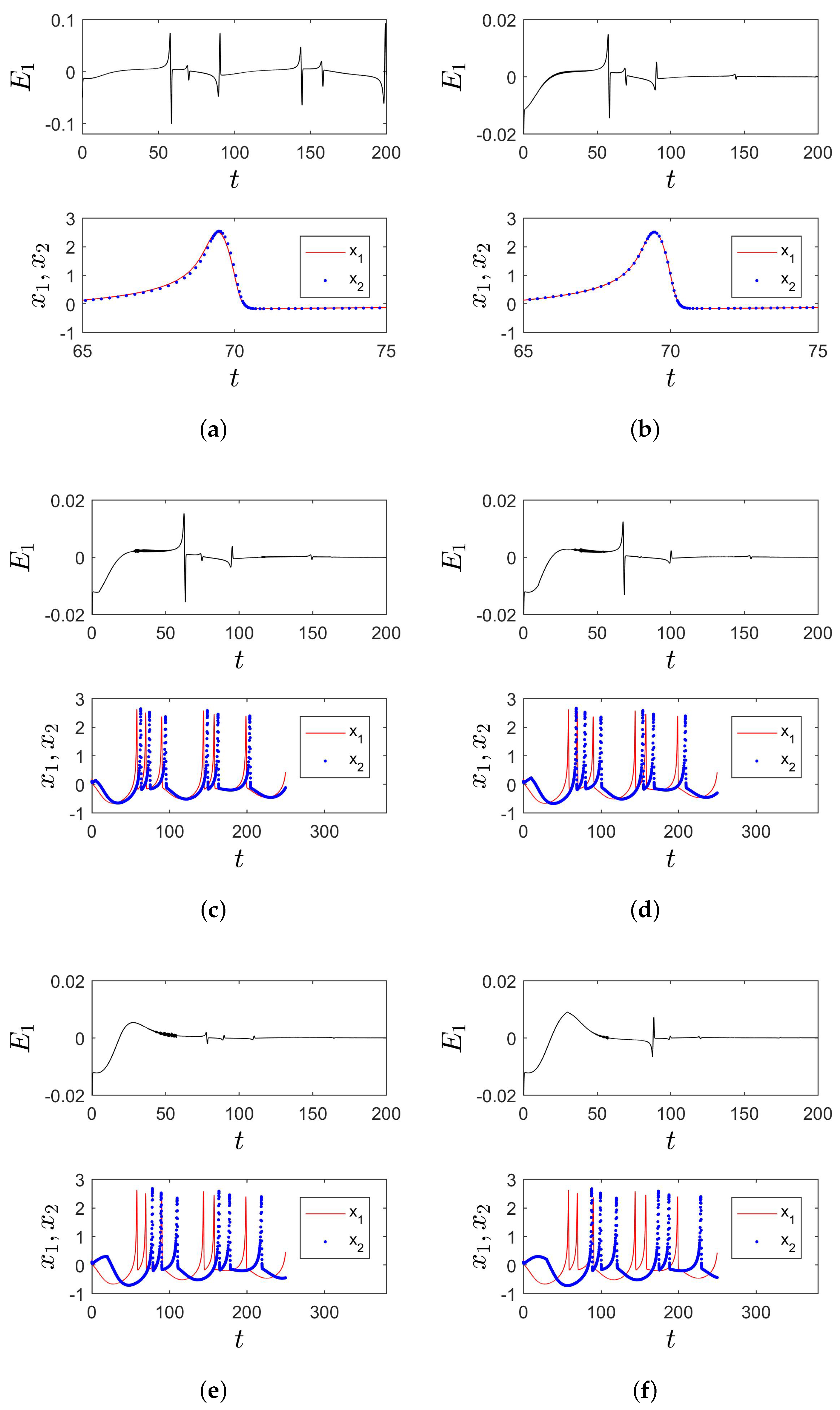
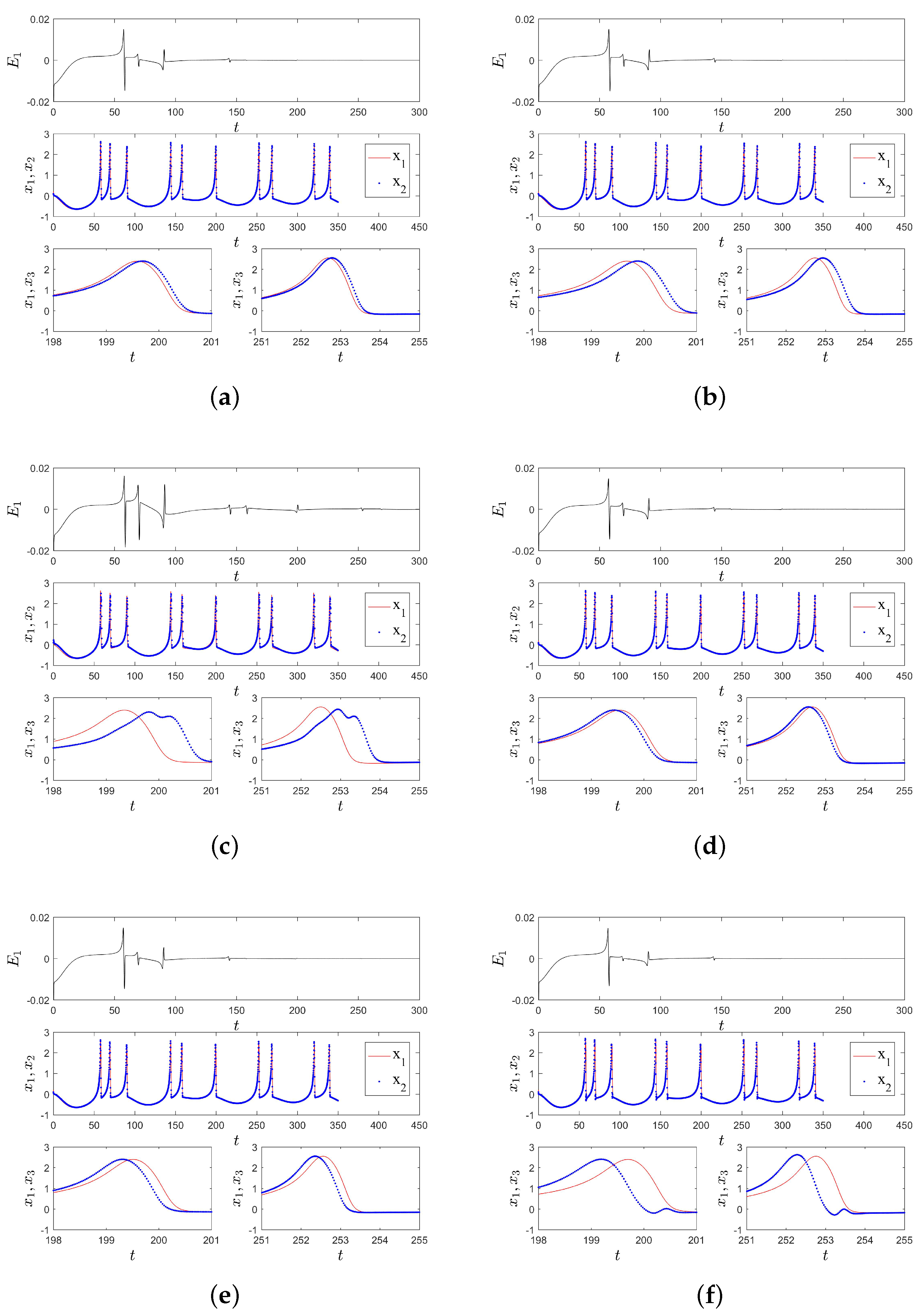
4. GS between Two HR Neurons

A HR neuron is described by the following equation of motion:
u ˙ = v a u 3 + b u 2 w + I e x t , v ˙ = c d u 2 v , w ˙ = r s 0 ( u x 0 ) r w ,
where u is the membrane potential, v is a recovery variable associated with fast current, and w represents a slowly changing adaptation current. a, b, c, d, s 0 , r, x 0 are parameters, and I e x t is the external current input. For simplicity, by letting x = u u 0 , y = v v 0 , and z = w w 0 , where ( u 0 , v 0 , w 0 ) is the equilibrium of System (25), System (25) becomes
x ˙ = a x 3 + ρ 1 x 2 + ρ 2 x + y z , y ˙ = d x 2 + ρ 3 x y , z ˙ = r ( s 0 x z ) ,
where ρ 1 = 3 a u 0 + b , ρ 2 = 3 a u 0 2 + 2 b u 0 , ρ 3 = 2 d u 0 , u 0 is the unique real root to equation a u 0 3 + ( d b ) u 0 2 + s 0 u 0 ( s 0 x 0 + c + I e x t ) = 0 . Consider two HR neurons described by System (26) have the following coupling form:
x ˙ 1 = a x 1 3 + ρ 1 x 1 2 + ρ 2 x 1 + y 1 z 1 , y ˙ 1 = d x 1 2 + ρ 3 x 1 y 1 , z ˙ 1 = r ( s 0 x 1 z 1 ) , x ˙ 2 = a x 2 3 + ρ 1 x 2 2 + ρ 2 x 2 + y 2 z 2 + α ( x 2 J ( x 1 ) ) , y ˙ 2 = d x 2 2 + ρ 3 x 2 y 2 , z ˙ 2 = r ( s 0 x 2 z 2 ) ,
where J ( x 1 ) is a continuous function of x 1 , and α represents the coupling strength. Similarly, we consider that System (27) has the property
lim t | | x 2 J ( x 1 ) | | = 0 .
Clearly, J ( x 1 ) can have the form of J ( x 1 ) = x 1 ( t τ ) , in which τ 0 is a delay.
From the auxiliary system approach, the auxiliary system corresponding to System (27) is given by
x ˙ 3 = a x 3 3 + ρ 1 x 3 2 + ρ 2 x 3 + y 3 z 3 + α ( x 3 J ( x 1 ) ) , y ˙ 3 = d x 3 2 + ρ 3 x 3 y 3 , z ˙ 3 = r ( s 0 x 3 z 3 ) .
According to the analysis in the last section, Condition (28) will be satisfied if
lim t | | x 2 x 3 | | = 0 .
By letting
E 1 = x 2 x 3 2 , E 2 = x 2 + x 3 2 ,
the response system and the auxiliary system in Systems (27) and (29) can be rewritten as
E ˙ 1 = a E 1 3 ( 3 a E 2 2 2 ρ 1 E 2 α ρ 2 ) E 1 + y 2 z 2 y 3 + z 3 2 , y ˙ 2 = d ( E 1 + E 2 ) 2 + ρ 3 ( E 1 + E 2 ) y 2 , z ˙ 2 = r [ s 0 ( E 1 + E 2 ) z 2 ] , E ˙ 2 = a E 2 3 ( 3 a E 1 2 α ρ 2 ) E 2 + ρ 1 ( E 1 2 + E 2 2 ) α J ( x 1 ) + y 2 z 2 + y 3 z 3 2 , y ˙ 3 = d ( E 2 E 1 ) 2 + ρ 3 ( E 2 E 1 ) y 3 , z ˙ 3 = r [ s 0 ( E 2 E 1 ) z 3 ] .
Then Condition (30) is equivalent to
lim t | | E 1 | | = 0 .
From the Laplace transform method used in the last section, the Laplace transform of E 1 can be given by
E ^ 1 = E 10 s 2 + φ 4 s + φ 5 s 3 + φ 1 s 2 + φ 2 s + φ 3 ( r + s ) [ M 1 + ( s + 1 ) M 2 ] s 3 + φ 1 s 2 + φ 2 s + φ 3 ,
where
φ 1 = r ρ 2 α + 1 , φ 2 = r ( 1 + s 0 ρ 2 α ) α ρ 2 ρ 3 , φ 3 = r ( s 0 α ρ 2 ρ 3 ) , φ 4 = ( r + 1 ) E 10 + y 20 z 20 y 30 + z 30 2 , φ 5 = r E 10 + r y 20 z 20 r y 30 + z 30 2 , M 1 = 2 d 0 + E 1 E 2 e s t d t , M 2 = 0 + [ a ( E 1 2 + 3 E 2 2 ) 2 ρ 1 E 2 ] E 1 e s t d t .
According to the analysis in the last section based on the theory of Volterra integral equations (Equations (17)–(19)), the condition that E 1 = 0 means the following polynomial (the denominator in the right-hand side of Equation (34))
s 3 + φ 1 s 2 + φ 2 s + φ 3
has no roots with positive real parts. That is,
φ 1 > 0 , φ 2 > 0 , φ 3 > 0 a n d φ 1 φ 2 > φ 3 .
Next, numerical simulations are performed to prove that the method to investigate GS proposed in this paper is valid even if the drive–response system has chaotic attractor. Here, a = 1.0 , b = 3.0 , c = 1.0 , d = 5.0 , s 0 = 4.0 , r = 0.013 , x 0 = 1.6 , and I e x t = 3.0 . The two HR neurons in System (27) with α = 0 exhibit burst-spike chaotic behavior. From Condition (36), the functional relation x 2 = x 1 ( t τ ) appears between two HR neurons when α < 1.129 . To demonstrate the validity of the condition, α = 0.9 and α = 1.3 are taken to perform the numerical simulations of System (27), respectively. The initial conditions are given by x 1 ( t ) = 0.2 , t ( τ , 0 ] , y 1 ( 0 ) = 0.1 , z 1 ( 0 ) = 0.2 , x 2 ( 0 ) = 0.1 , y 2 ( 0 ) = 0.1 , z 2 ( 0 ) = 0.1 , x 3 ( 0 ) = 0.2 , y 3 ( 0 ) = 0.2 , and z 3 ( 0 ) = 0.1 . The numerical results are presented in Figure 3. From Figure 3a,b, condition α < 1.129 is efficient to guarantee the appearance of GS between two HR neurons in System (27). As shown in Figure 3b–f, the condition is valid for any value of τ , which means that the functional relation x 2 = x 1 ( t τ ) is achieved when α = 1.3 .
Similarly, consider
J ( x 1 ) = x 1 ( t ) d x 1 d t τ + 1 2 ! d 2 x 1 d t 2 τ 2 1 3 ! d 3 x 1 d t 3 τ 3 Q ( x 1 , y 1 , z 1 , τ ) ,
in System (27). From Equation (27), one has
d x 1 d t = a x 1 3 + ρ 1 x 1 2 + ρ 2 x 1 + y 1 z 1 , d 2 x 1 d t 2 = ( 3 a x 1 2 + 2 ρ 1 x 1 + ρ 2 ) d x 1 d t d x 1 2 + ρ 3 x 1 y 1 r ( s 0 x 1 z 1 ) , d 3 x 1 d t 3 = ( 3 a x 1 2 + 2 ρ 1 x 1 + ρ 2 ) d 2 x 1 d t 2 + 2 ( ρ 1 3 a x 1 ) ( d x 1 d t ) 2 + ( ρ 3 2 d x 1 r s 0 ) d x 1 d t + r 2 ( s 0 x 1 z 1 ) + d x 1 2 ρ 3 x 1 + y 1 .
From Figure 4a,b,d,e, the functional relation x 2 = x 1 ( t τ ) is reached between two HR neurons in System (27) with J ( x 1 ) = Q ( x 1 , y 1 , z 1 , τ ) for a small value of τ when α = 1.3 . When the value of τ increases (decreases) to τ = ± 0.5 , the functional relation x 2 = x 1 ( t τ ) cannot be satisfied in System (27) (Figure 4c,f). Compared with the case of two FHN neurons, more higher order terms of τ need to keep the functional relation between two HR neurons. It is feasible to construct a coupling function using the current signal of an HR neuron to predict its future signal or make its past signal reappear.

5. Conclusions

In this paper, a new method is proposed to investigate GS between two identical FHN and HR neurons with unidirectional coupling. Based on the auxiliary system approach, GS between the drive and response systems occurs if synchronization between the response and auxiliary systems is achieved. Different from other researchers, the synchronization problem is solved in this paper by using the Laplace transform and the convolution theorem, as well as the iterative method in the theory of Volterra integral equations. An analytical criterion is ultimately obtained to determine the occurrence of GS in the drive–response system. Numerical simulations are carried out for the drive–response system consisting of two FHN neurons and two HR neurons to prove the correctness and efficiency of the analytical criterion.
The functional relation in GS between two identical neurons is very special, referring to the situation where there is a time difference between the trajectories of the drive and response systems. Furthermore, the time difference has nothing to do with the GS condition, which depends on the coupling function between two neurons. According to Taylor’s expansion, one can easily construct a coupling function between two neurons by using the current signal of the drive system to predict its future signal or make its past signal reappear. Numerical simulations show that the coupling function based on Taylor’s expansion is valid to not only the FHN neural system exhibiting periodic spike behavior but also the HR neural system exhibiting burst-spike behavior.
Drive–response synchronization techniques had typical applications in designing secure communication systems because they are typically similar to the transmitter–receiver structure. Some methods designing chaos-based secure communication systems require real-time synchronization between drive and response systems. However, time delay in signal transmission between the transmitter–receiver structure is inevitable. Our study provides an approach to predict future signals of a chaotic system based on its current signal, which may be used to overcome the problem of delay of signal propagating channels.

Author Contributions

Conceptualization, B.Z.; methodology, B.Z.; software, R.L.; investigation, B.Z. and R.L.; writing—original draft preparation, B.Z. and R.L.; writing—review and editing, B.Z.; visualization, R.L.; supervision, B.Z.; project administration, B.Z.; funding acquisition, B.Z. All authors have read and agreed to the published version of the manuscript.

Funding

This research was funded by the National Natural Science Foundation of China grant number 11672185.

Institutional Review Board Statement

Not applicable.

Informed Consent Statement

Not applicable.

Data Availability Statement

The study did not report any data.

Acknowledgments

The authors greatly appreciate the anonymous referees for their valuable suggestions and questions. The authors gratefully acknowledge the financial support from the National Natural Science Foundation of China grant number 11672185.

Conflicts of Interest

The authors declare no conflict of interest.

References

  1. Arenas, A.; Díaz-Guilera, A.; Kurths, J.; Moreno, Y.; Zhou, C. Synchronization in complex networks. Phys. Rep. 2008, 18, 037111. [Google Scholar] [CrossRef] [Green Version]
  2. Boccaletti, S.; Kurths, J.; Osipov, G.; Valladares, D.L.; Zhou, C.S. The synchronization of chaotic systems. Phys. Rep. 2002, 366, 1–101. [Google Scholar] [CrossRef]
  3. Ding, X.L.; Gu, H.G.; Jia, B.; Li, Y.Y. Anticipated synchronization of electrical activity induced by inhibitory autapse in coupled Morris-Lecar neuron model. Acta Phys. Sin. 2021, 70, 218701. [Google Scholar]
  4. Kim, S.-Y.; Lim, W. Effect of inhibitory spike-timing dependent plasticity on fast sparsely synchronized rhythms in a small-world neuronal network. Neural Netw. 2018, 106, 50–66. [Google Scholar] [CrossRef] [PubMed] [Green Version]
  5. Zhao, X.; Liu, J.; Zhang, F.F.; Jiang, C.M. Complex generalized synchronization of complex-variable chaotic systems. Eur. Phys. J. 2021, 230, 2035–2041. [Google Scholar] [CrossRef]
  6. Moskalenko, O.I.; Koronovskii, A.A.; Plotnikova, A.D. Peculiarities of generalized synchronization in unidirectionally and mutually coupled time-delayed systems. Chaos Soliton Fractals 2021, 148, 111031. [Google Scholar] [CrossRef]
  7. Moskalenko, O.I.; Koronovskii, A.A.; Selskii, A.O.; Evstifeev, E.V. On multistability near the boundary of generalized synchronization in unidirectionally coupled chaotic systems. Chaos 2021, 31, 083106. [Google Scholar] [CrossRef]
  8. Jiang, G.P.; Tang, W.K.S. A global synchronization criterion for coupled chaotic systems via unidirectional linear error feedback approach. Int. J. Bifurc. Chaos 2011, 12, 2239–2253. [Google Scholar] [CrossRef] [Green Version]
  9. Kocarev, L.; Parlitz, U. General approach for chaotic synchronization with applications to communication. Phys. Rev. Lett. 1995, 74, 5028–5031. [Google Scholar] [CrossRef]
  10. Chua, L.O.; Kocarev, L.; Eckert, K.; Itoh, M. Experimental chaos synchronization in Chua’s circuit. Int. J. Bifurc. Chaos 2011, 2, 705–708. [Google Scholar] [CrossRef]
  11. Abarbanel, H.D.I.; Rulkov, N.F.; Suschik, M.M. Generalized synchronization of chaos: The auxiliary system approach. Phys. Rev. E 1996, 53, 4528–4535. [Google Scholar] [CrossRef] [PubMed] [Green Version]
  12. Pecora, L.M.; Carroll, T.L. Master stability functions for synchronized coupled systems. Phys. Rev. Lett. 1998, 80, 2109–2112. [Google Scholar] [CrossRef]
  13. Wouapi, K.M.; Fotsin, B.H.; Louodop, F.P.; Feudjio, K.F.; Njitacke, Z.T.; Djeudjo, T.H. Various firing activities and finite-time synchronization of an improved Hindmarsh-Rose neuron model under electric field effect. Cogn. Neurodyn. 2020, 14, 375–397. [Google Scholar] [CrossRef]
  14. Zhou, X.; Xu, Y.; Wang, G.; Jia, Y. Ionic channel blockage in stochastic Hodgkin-Huxley neuronal model driven by multiple oscillatory signals. Cogn. Neurodyn. 2020, 14, 569–578. [Google Scholar] [CrossRef] [PubMed]
  15. Rehak, B.; Lynnyk, V. Synchronization of a Network Composed of Stochastic Hindmarsh-Rose Neurons. Mathematics 2021, 9, 2625. [Google Scholar] [CrossRef]
  16. Sharma, S.K.; Mondal, A.; Mondal, A.; Upadhyay, R.K.; Ma, J. Synchronization and Pattern Formation in a Memristive Diffusive Neuron Model. Int. J. Bifurc. Chaos 2021, 31, 2130030. [Google Scholar] [CrossRef]
  17. Boaretto, B.R.R.; Budzinski, R.C.; Rossi, K.L.; Manchein, C.; Prado, T.L.; Feudel, U.; Lopes, S.R. Bistability in the synchronization of identical neurons. Phys. Rev. E 2021, 104, 024204. [Google Scholar] [CrossRef]
  18. Wang, J.Y.; Yang, X.L.; Sun, Z.K. Suppressing bursting synchronization in a modular neuronal network with synaptic plasticity. Cogn. Neurodyn. 2018, 12, 625–636. [Google Scholar] [CrossRef]
  19. Sun, X.; Xue, T. Effects of time delay on burst synchronization transition of neuronal networks. Int. J. Bifurc. Chaos 2018, 28, 1850143. [Google Scholar] [CrossRef]
  20. Kim, S.-Y.; Lim, W. Cluster burst synchronization in a scale-free network of inhibitory bursting neurons. Cogn. Neurodyn. 2020, 14, 69–94. [Google Scholar] [CrossRef] [Green Version]
  21. Semenov, D.M.; Fradkov, A.L. Adaptive synchronization in the complex heterogeneous networks of Hindmarsh-Rose neurons. Chaos Solitons Fractals 2021, 150, 111170. [Google Scholar] [CrossRef]
  22. Wang, Y.H.; Li, X.D.; Song, S.J. Exponential synchronization of delayed neural networks involving unmeasurable neuron states via impulsive observer and impulsive control. Neurocomputing 2021, 441, 13–24. [Google Scholar] [CrossRef]
  23. Hodgkin, A.; Huxley, A. A quantitative description of membrane current and its application to conduction and excitation in nerve. Bull. Math. Biol. 1990, 52, 25–71. [Google Scholar] [CrossRef]
  24. Fitzhugh, R. Mathematical models of threshold phenomena in the nerve membrane. Bull. Math. Biophys. 1955, 17, 257–278. [Google Scholar] [CrossRef]
  25. Hindmarsh, J.L.; Rose, R.M. A model of neuronal bursting using three coupled first order differential equations. Proc. R. Soc. London Ser. B Biol. Sci. 1984, 221, 87–102. [Google Scholar]
  26. Xu, L.; Qi, G.Y.; Ma, J. Modeling of memristor-based Hindmarsh-Rose neuron and its dynamical analyses using energy method. Appl. Math. Model. 2022, 101, 503–516. [Google Scholar] [CrossRef]
  27. Kim, S.-Y.; Lim, W. Effect of spike-timing-dependent plasticity on stochastic burst synchronization in a scale-free neuronal network. Cogn. Neurodyn. 2018, 12, 315–342. [Google Scholar] [CrossRef] [PubMed]
  28. Nohel, J.A. Some problems in nonlinear Volterra integral equations. Bull. Am. Math. Soc. 1962, 68, 323–330. [Google Scholar] [CrossRef] [Green Version]
Figure 1. Synchronization errors and functional relation between u 1 and u 3 in System (3) with H ( u 1 ) = u 1 ( t τ ) and (a) k = 0.19 , τ = 0 , (b) k = 0.7 , τ = 0 , (c) k = 0.7 , τ = 5 , (d) k = 0.7 , τ = 10 , (e) k = 0.7 , τ = 20 , and (f) k = 0.7 , τ = 30 .
Applsci 11 11774 g001
Figure 2. Synchronization errors and functional relation between u 1 and u 3 in System (3) with H ( u 1 ) = G ( u 1 , u 2 , τ ) , k = 0.7 and (a) τ = 0.5 , (b) τ = 1 , (c) τ = 2 , (d) τ = 0.5 , (e) τ = 1 , and (f) τ = 2 .
Applsci 11 11774 g002
Figure 3. Synchronization errors and functional relation between x 1 and x 2 in System (27) with J ( x 1 ) = x 1 ( t τ ) and (a) α = 0.8 , τ = 0 , (b) α = 1.3 , τ = 0 , (c) α = 1.3 , τ = 5 , (d) α = 1.3 , τ = 10 , (e) α = 1.3 , τ = 20 , and (f) α = 1.3 , τ = 30 .
Applsci 11 11774 g003
Figure 4. Synchronization errors and functional relation between x 1 and x 2 in System (27) with J ( x 1 ) = Q ( x 1 , y 1 , z 1 , τ ) , α = 1.3 and (a) τ = 0.1 , (b) τ = 0.2 , (c) τ = 0.5 , (d) τ = 0.1 , (e) τ = 0.2 , and (f) τ = 0.5 .
Applsci 11 11774 g004
Publisher’s Note: MDPI stays neutral with regard to jurisdictional claims in published maps and institutional affiliations.

