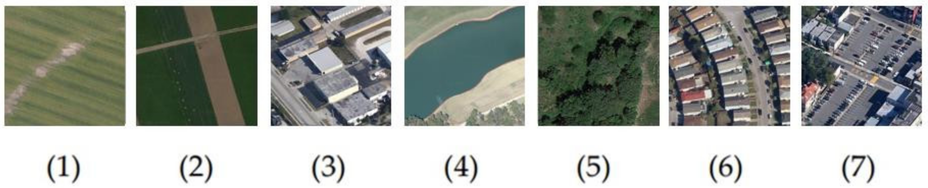
Article

Integrating Image Quality Enhancement Methods and Deep Learning Techniques for Remote Sensing Scene Classification

by
Sheng-Chieh Hung
1,†,
Hui-Ching Wu
2,† and
Ming-Hseng Tseng
1,3,4,*
1
Master Program in Medical Informatics, Chung Shan Medical University, Taichung 402, Taiwan
2
Department of Medical Sociology and Social Work, Chung Shan Medical University, Taichung 402, Taiwan
3
Department of Medical Informatics, Chung Shan Medical University, Taichung 402, Taiwan
4
Information Technology Office, Chung Shan Medical University Hospital, Taichung 402, Taiwan
*
Author to whom correspondence should be addressed.
These authors contributed equally to this work.
Appl. Sci. 2021, 11(24), 11659; https://doi.org/10.3390/app112411659
Submission received: 4 November 2021 / Revised: 1 December 2021 / Accepted: 4 December 2021 / Published: 8 December 2021
(This article belongs to the Special Issue Advances in Deep Learning III)

Abstract

:
Through the continued development of technology, applying deep learning to remote sensing scene classification tasks is quite mature. The keys to effective deep learning model training are model architecture, training strategies, and image quality. From previous studies of the author using explainable artificial intelligence (XAI), image cases that have been incorrectly classified can be improved when the model has adequate capacity to correct the classification after manual image quality correction; however, the manual image quality correction process takes a significant amount of time. Therefore, this research integrates technologies such as noise reduction, sharpening, partial color area equalization, and color channel adjustment to evaluate a set of automated strategies for enhancing image quality. These methods can enhance details, light and shadow, color, and other image features, which are beneficial for extracting image features from the deep learning model to further improve the classification efficiency. In this study, we demonstrate that the proposed image quality enhancement strategy and deep learning techniques can effectively improve the scene classification performance of remote sensing images and outperform previous state-of-the-art approaches.

1. Introduction

With the continuous development of science and technology, the image quality achieved by air cameras, mobile phones, and other camera equipment has progressively improved. Additionally, the information that can be obtained from the image is richer in detail. When remote sensing images are used for deep learning model training, the proper categorization of scenes is an important step in understanding the classification of remote sensing images. Remote sensing image scene classification tasks can be applied in various fields [1,2] such as disaster prevention and relief, smart city planning, land covering, and land change detection. Thus, the automatic classification of a large amount of remote sensing image data is a crucial study topic [3].
For the improvement of the image data, the use of various methods of enhancement processing may provide a higher level of image characteristics and assist in reinforcing the image features of the neural network model in the subsequent phase. For image processing, most of the existing methods are to directly crop the original image into the model training. However, for some images with poor quality, the details and contrast are often not satisfactory with the requirements after multiple feature extractions. Consequently, it is difficult to achieve good results with the scene classification task. Using the Sobel edge detection algorithm and Gaussian smoothing function to identify the relevant region in an image, Bhowmik et al. [4] suggested region-based processing to discard background information and obtain a faster converge for deep learning model training. The image quality assessment method is used to quantify the level of image accuracy, which can be classified as subjective and objective methods. The subjective method is based on the user’s perception of the image, whereas the objective method is based on the mathematical calculation model for image quality prediction. Varga [5] extracted visual features by attaching global average pooling layers to multiple inception modules of an ImageNet database pre-trained convolutional neural network for no-reference image quality assessment.
Within the model of the deep neural network of supervised learning, if we can figure out where the distinctive feature texture of the region in the image, it will be a help for predicting and would provide significant assistance in the model development. Thus, using explainable artificial intelligence (XAI) technology is very useful for image analysis of model training, which includes understanding the reasonable and interpretable relationship between model prediction and image characteristics [6,7]. When we can explain how the model performs task classification analysis, we can use it to assess whether the model decisions are reasonable. We can modify the model to ensure its reliability, thereby utilizing an interpretable feature correction method to further improve the accuracy of model training. We previously proposed a deep CNN architecture (i.e., RSSCNet) [8] for remote sensing scene classification tasks, and then used the Local Interpretable Model-Agnostic Explanation (LIME) [9] to analyze misclassified cases. Finally, we confirmed that the image quality will affect the classification performance of deep learning models.
The primary difference between this and the previous study [8] is that this study proposes an automated image quality enhancement strategy as a preprocessing procedure that can improve the RSSCNet model’s generalization ability. However, the previous study [8] only performed a manual image correction process for the four misclassified images by the RSSCNet model. This manual image correction process [8] is postprocessing, labor-intensive, and time-consuming procedure.
The main contribution of this study is to explore the impact of different image quality improvement methods on the classification results of deep learning models. Through image processing procedures such as noise reduction, sharpening, partial color area uniformization, and color channel adjustment, a set of automated image quality methods is proposed. Our objective is to enhance the current method and use XAI technology to analyze and demonstrate the importance of the image quality improvement strategy recommended by this study for building a deep learning model with high generalization performance.

2. Materials and Methods

2.1. Dataset

This study uses two image datasets: the RSSCN7 [10] and WHU-RS19 image datasets [11]. Table 1 summarizes the characteristics of these datasets.
The RSSCN7 image dataset is a public dataset released by Wuhan University in 2015. There are seven different scene categories: includes grassland, fields, industrial areas, rivers/lakes, forests, residential areas, and parking lots. The overall dataset contains a total of 2800 images. Each of these categories contains 400 images with four different telemetry sampling rates, and the sizes of all images are 400 × 400 pixels, as shown in Figure 1.
The WHU-RS19 image dataset is extracted from satellite images derived from Google Earth. The spatial resolution of these satellite images is up to 0.5 m, and the spectral bands are red, green, and blue (RGB). The image dataset contains 19 scene categories, which includes airports, beaches, bridges, commercial areas, deserts, farmland, football fields, forests, industrial areas, grasslands, mountains, parks, parking lots, ponds, ports, train stations, residential areas, rivers, and viaducts; there are about 50 images corresponding to each category. The entire data set has a total of 1,005 images, and the original image sizes are 600 × 600 pixels, as shown in Figure 2.

2.2. Image Quality Enhancement Strategy

To explore the effect of different image quality enhancement strategies on the performance of the deep learning classification model, this study uses a series of pixel enhancement methods to validate the image quality improvement of the original image dataset and discusses the noise reduction, sharpening, partial color uniformity, and color to improve the effectiveness of image processing procedures such as channel adjustment. Finally, a set of optimized image quality enhancement methods was developed. The entire research process is shown in Figure 3.

2.2.1. Image Denoising and Sharpening Processing

This study first analyzes the effectiveness for the testing of image denoising and sharpening processing. Unsharp masking (USM) is a commonly used technique to sharpen the edge of the image; it can improve the contrast of image edge detail. In this study, we subtract the Gaussian smoothed version from the original image and retain the value of the constant area in a weighted manner to realize the sharpening function, when X is the enhanced image, X is the original image, Y is the Gaussian smoothed image, and a and b are the weights of images, the formula is expressed as follows:
X = a X + b Y
We use the Gaussian Blur function to generate a Gaussian blurred image as an USM, and then we mix the original image with the blurred image in a ratio of 1.5: −0.5 to make the blurred image perform the reverse operation. The unsharp mask and the original image are combined to produce an image that is more obvious than the original image edge, which strengthens the model’s ability to detect the edges during training. The original image and the sharpened image are compared, as shown in Figure 4.
Next, we validate the image data with the sharpening processing. The sharpening method is from the Non-local Means Denoising algorithm [12], which is an image noise reduction algorithm. When compared with the local algorithms such as the Gaussian Blur and anisotropic diffusion, the Non-local Means Denoising algorithm only uses the range near the target pixel to smoothen the image and remove the image noise. In the local averaging algorithm, each target pixel is defined as a block of a specified size, and all pixels in the entire image are weighted according to the similarity between the surrounding block of the pixel and the target pixel block. Similar block images are averaged, so that the processed image has less noise, and the retained image texture is more evident. Although this denoising method will take more time, the effect of denoising is better, thereby obtaining the edge details of the image with smaller loss. In the set block size, this paper uses 16 × 16 as the average pixel range size, as shown in Figure 5.

2.2.2. Image Color Enhancement Processing

In this study, the three methods described below will be tested for color enhancement of images: Contrast Limited Adaptive Histogram Equalization (CLAHE), Multi-Scale Retinex with Color Restoration (MSRCR), and Multi-Scale Retinex with chromaticity preservation (MSRCP).
First, we evaluate the CLAHE [13] method to perform the image quality tests. The histogram equalization method is different from the traditional image processing technology; it calculates the image histogram, then crops the histogram and perform equalization. Increasing the overall contrast of the image during equalization will also increase the noise contrast in the input image. Through the adaptive histogram equalization method, the input image is divided into small image fragments, which are enhanced by applying CLAHE to the regional fragments instead of the entire image; the mathematical formation for the histogram limit of each region is given as:
β = M N 1 + α 100 S m a x 1
where M is the pixels in each region, N is the dynamic range in region, S m a x is the maximum allowable slope, and α is the clip factor set between 0 to 100. Using this formula, we can obtain the clip limit, β , which limits the change in image contrast.
Next, we use the bilinear interpolation to seamlessly stitch the generated adjacent image blocks to limit the contrast of the uniform area, thereby avoiding an increase in noise to produce better image quality output. It can be seen from Figure 6 that the light, shadow, and contrast of the forest image have been improved after CLAHE correction, and it is easier to recognize with the human eye.
Then, we assess the MSRCR; this method is based on the Multi-Scale Retinex (MSR) [14]. In the MSR enhancement process, the image may be distorted due to the increase of noise, and the color of the local details of the image may be distorted. Hence, the true color of the object cannot be shown, and the overall visual effect will be worse. To deal with this problem, Jobsonet et al. [15] proposed to complete the algorithm with color restoration steps. When adding the color restoration step into the MSR method, the color restoration factor is used to adjust the defect of the color distortion caused by the contrast enhancement of the local area of the image. They proposed modifying the MSR output by multiplying the MSR output by the color restoration function of the chroma to adjust the difference between the three-color channels in the original image. We highlight the information in the relatively dark area and eliminate the defect of the image color distortion. After processing, the local contrast of the image is improved, and the brightness will be similar to the actual scenery; the algorithm for the MSRCR method can be is given below:
R M S R C R i x , y = C i x , y R M S R i x , y
C i x , y = f I i x , y
The function that provides best overall color restoration is below, where β is a gain constant, α controls the strength of the nonlinearity:
C i x , y = β log α I i x , y
When we review the image with our visual perception, the image appears more realistic. Figure 7 displays the original image and the image of the industrial area corrected by MSRCR. It can be found that the MSRCR method corrected the white balance and color problems in the original image. In addition, this study will simultaneously test the MSRCP without color restoration but only retain the chromaticity.

2.3. XRAI Technology

XRAI technology [16] combines patch identification [9] and the integrated gradients [17]. XAI uses the interpretable performance of the model to assist with the following: extraction of distinctive textures and details from a large number of images, understanding how to perform image classification analysis with appropriate decision-making between images and models, and the determination of the images captured in the model. Whether the texture feature is reasonable, we evaluate the correctness of the feature area in the classification decision and improve the image quality when the prediction is wrong, thereby ensuring the reliability of the classification. The XRAI technology used in this study divides the image into many small overlapping areas, and then use the integrated gradient to obtain the contribution of the non-zero gradient of the unsaturated zone to the importance of model decision-making. The analysis results of the hot zone map can show the significant area that has the greatest impact on the model decision-making, rather than a single pixel, as shown in Figure 8. XRAI’s use of this larger significant area can often yield better interpretation, and we can directly observe the effects of this interpretation of the image feature texture after training.

2.4. Deep Learning Model

The neural network model used in this study is illustrated in Figure 9, utilizing the RSSCNet method [8]. The main research direction in this study is to propose CNN telemetry scene classification network architecture and use transfer learning technology to modify the deep learning model to obtain better accuracy. There are two convolutional layers in RSSCNet: a global average pooling layer and three batch normalization layers [18]. The activation function of the convolutional layers is ELU [19]. There are two fully connected layers and a dropout layer; the filter size in the convolutional layer is 3 × 3 pixels, the dropout rate is set to 0.5, the fully connected layer uses the L1 regularization, and the parameter is set to 0.01.

3. Results

The training equipment in this research is the Windows 10 system operating platform, and the core processor used in the hardware configuration is AMD Ryzen™ 3 PRO 4350G with 32 GB random access memory, and the NVIDIA GeForce GTX3060 12G graphics card is used for the deep learning model training. The software uses the Python programming language for development and design using Anaconda 4.4.10 (Python 3.8). The Tensorflow software package used for model training is Tensorflow-GPU 2.4 version, and the CUDA version is 11.1. In all experiments, the length and width of the image are both set to 256 pixels. This study utilizes the training set size designed based on related research [8]. For the RSSCN7 image dataset, 50% of the training dataset is used, and for the WHU-RS19 dataset, 40% of the training dataset is used.
In the experiment, 300 epochs of training will be carried out uniformly, and a two-stage training strategy will be used to deliver a cyclical learning rate. In the first stage, the SGD optimizer will be used to add the Nesterov momentum learning rates between 0.001 and 0.00001. We carry out one cycle of the cyclic learning strategy, and the second stage uses the Adam optimizer to perform the decremental cyclic learning rates between 0.0001 and 0.00001 for training, as shown in Figure 10.
In this study, the training accuracy, test accuracy, overall accuracy, and test correct cases were used for the performance evaluation of the model classification; the results of the overall accuracy are compared to those obtained in other studies. The overall accuracy is the ratio between the model’s correct predictions on full datasets and the overall numbers. The overall accuracy ranged from 0 to 1, with a number closer to 1 indicating that the model has better classification performance.

3.1. Effects of Image Denoising Methods

This study first discusses the difference in the impact of different denoising and sharpening image correction methods on model training. In addition to using the original image for training, we compare the application of the following methods: (1) the Gaussian Blur USM added to the original image, (2) the fastNlMeans Denoising Colored denoising method, (3) fastNlMeans Denoising Colored using USM added to the original image, and (4) the simultaneous use of the Gaussian Blur and fastNlMeans Denoising Colored added as a mask to the original image.
After all methods have undergone 300 iterations of training, the results of the RSSCN7 image dataset that are obtained are shown in Table 2; the table shows the test accuracy and the number of correct classifications of the test images. Table 1 shows the image denoising effect. The best denoising method is adding the fastNlMeans USM to the original image to achieve the best accuracy. When compared with the training results of the original image dataset with the total number of 1400 test image predictions, it is found that the number of correctly predicted images has increased by 12.
In addition, we tested five methods on the WHU-RS19 image dataset. From Table 3, it can be seen that the correction method is realized when the original image is added to the fastNlMeans Denoising Colored mask to obtain the best accuracy. When compared with the original image prediction results, we realize that the number of correct predictions of three images can be improved; thus, we ascertain that the use of the fastNlMeans Denoising Colored mask method can improve the accuracy of the model prediction.

3.2. Effects of Image Enhancement Methods

Next, we discuss the effectiveness of using different color correction methods. The experiment uses three different correction methods: CLAHE, MSRCR, and MSRCP. All methods were trained by 300 epochs; the results of the RSSCN7 image dataset that were obtained are shown in Table 4. The table shows the test accuracy and the correct number of test images. It can be seen from Table 4 that the best test accuracy can be obtained by using the CLAHE correction method. When compared with the training results of the original image dataset, the total number is 1400. When considering the test image prediction, the number of correctly predicted images increased by 12.
Furthermore, we compare the three methods utilizing the WHU-RS19 image dataset. It can be seen from Table 5 that the best accuracy can be obtained with the CLAHE correction method, and when compared with the original image dataset, the number of correct images also improved.

3.3. Effects of Color Spaces

After discussing the CLAHE image color fix method, we additionally validated whether the application of the different color spaces in relation to the correction method will have other different degrees of improvement. Therefore, we use the HSV and LAB, which are two common color space methods to convert the image. After the color space conversion, the CLAHE method is used for correction, and then the training prediction is performed. Table 6 shows the results of RSSCN7 dataset that use of LAB or HSV color spaces are not any better than the RGB color fix image for the CLAHE prediction.

3.4. Scene Classification Performance

Finally, we combine the best denoising sharpening method and the color correction method to improve the image quality. The two best methods (Denoising Sharpen and CLAHE) are simultaneously corrected, and then the images are trained and predicted. Figure 11 shows the curves of the two-stage training process. As can be observed, the accuracy and loss for both training and validation sets are in a good performance. The overall execution time of the model training process of RSSCN7 dataset is 3085 s using an NVIDIA GeForce GTX3060 graphics card.
Table 7 shows the prediction performance of the RSSCN7 dataset; the test accuracy is increased from 0.95 to 0.965 using the proposed method compared to the training results of the original image dataset, and the number of images that are accurately predicted is increased by 21.
Additionally, we compared this method using the WHU-RS19 image dataset. The above method can also be obtained for better model prediction accuracy when compared to the original image training dataset. Figure 12 shows the model training history using the proposed method in the study, with the results confirming that the model training process is in a good performance. Using an NVIDIA GeForce GTX3060 graphics card, the overall execution time of the model training process of WHU-RS19 dataset is 1075 s.
Table 8 shows the prediction performance of the WHU-RS19 dataset. Using the proposed method in this study, the test accuracy is increased from 0.9768 to 0.9801 compared with the training results of the original image dataset.
Table 9 lists a comparative evaluation against several state-of-the-art classification methods using the RSSCN7 dataset classification, including the proposed method. With 20% and 50% training ratios, our proposed methods achieved the best overall accuracy for different training ratios.
Table 10 shows the results for the WHU-RS19 dataset; the proposed method outperforms other existing state-of-the-art methods, regardless of the training ratio.

4. Discussion

After correcting the image dataset by different correction methods in this study, it can be observed from the training results that through noise reduction, sharpening, and partial image enhancement, the images are processed through a consistent pixel enhancement method to achieve an automated method for optimal image quality. The automated quality enhancement strategy helps to improve the accuracy of prediction. When accurate and effective corrections are made, this process can be used to strengthen model training to achieve better classification accuracy.
In addition to discussing the different image correction methods, this study also hopes to yield an understanding of how the image feature texture enhancement is performed. Therefore, we use XRAI to visualize the feature regions of the hot zone map with the best prediction results, using this technology to perform an analysis of river/lake images in the RSSCN7 image dataset. As shown in Figure 13, the heatmap areas in the original image are concentrated on both sides, and the main feature block cut outs are distributed on the outer houses, which can explain the reason for the incorrect selection of the industry category. However, after fixing by noise sharpening and color correction, the hot zone moves to the central area, and the cropped main feature area also returns to the inner side of the lake, and then the correct classification category is obtained in the revised prediction. Figure 14 is also a river/lake image but was determined to be an incorrect field. After correction processing, the edge depth of the lakeside became strengthened and more evident. We can see the characteristic heatmap generated by XRAI, which is the primary focus area. The piece of land from the original outer edge was revised to the inner edge of the center of the lake. We can understand the basis for the image classification determination and the reason for accurate correction.
In addition, the error in the predicted parking lot images in the RSSCN7 image dataset was reviewed via XRAI analysis. As shown in Figure 15, the hot area in the original image did not capture the car grid of the parking lot, and only focused on the side eaves and trees along the street, which were strengthened after correction. The light and shadow of the edge of the car grid makes the parking lot grid more evident. Comparing with Figure 15a, it can be seen that the characteristic hot zone of XRAI contains a large number of parking lot grids from Figure 15b, and finally, the correct classification category is obtained in the revised prediction.
In this study, XRAI is used to visualize the heatmap based on the model prediction. We try to understand where the feature texture in the image has an effective basis for decision-making. Additionally, we evaluate the image to understand the feature texture of the image block and verify the correlation of the model prediction category. When considering the transfer of the salient feature position and the basis for the analysis and determination of the auxiliary verification using the image correction method, we can improve the model prediction under the condition of intelligibility and obtain better prediction accuracy.
Table 9 and Table 10 show the comparison of the overall performance on RSSCN7 and WHU-RS19 datasets. The performance of the proposed method in this study is better than the existing state-of-the-art approaches. This is because these existing methods exclusively applied original images for model training. However, this study adopts an image quality enhancement strategy in the deep learning model training. This image preprocessing method can enhance the input images’ quality, train the deep learning model to extract more effective image features, and improve the deep learning model’s overall performance.

5. Conclusions

Our research proposes a set of optimal image quality enhancement strategies after conducting multiple sets of experiments through different combinations of image processing procedures such as noise reduction, sharpening, partial image color area homogenization, and color channel adjustment. After testing two public remote sensing scene image datasets on scene image classification task, it was shown that the image quality enhancement strategy proposed in this study can effectively improve the generalization performance of the deep learning model after training.
This study uses the locally interpretable XRAI technology to analyze the significant image location difference before and after the image quality enhancement strategy of the original misclassified case. It also verifies the automated image quality enhancement strategy proposed in this study, which can assist in training the deep learning model to find the location of the image feature texture of the correct category, allowing the accuracy of the model to be further improved.
Additionally, our objective is to develop a supervised deep learning model with high generalization performance and well-designed model architecture, thereby improving the data quality of the image dataset, which is an equally important factor.
In future work, we will apply region-based processing [4] to eliminate background information and obtain faster convergence for model training and inference.

Author Contributions

Conceptualization, M.-H.T. and S.-C.H.; acquisition of data, M.-H.T. and S.-C.H.; analysis and interpretation of data, S.-C.H. and M.-H.T.; drafting of the manuscript, M.-H.T., S.-C.H. and H.-C.W. All authors have read and agreed to the published version of the manuscript.

Funding

This research was funded by the Ministry of Science and Technology, Taiwan, grant numbers MOST 109-2121-M-040-001 and MOST 110-2121-M-040-001.

Institutional Review Board Statement

Not applicable.

Informed Consent Statement

Not applicable.

Data Availability Statement

Data available on request.

Conflicts of Interest

All authors declare that there are no potential financial or non-financial conflict of interest.

References

  1. Rogan, J.; Chen, D. Remote sensing technology for mapping and monitoring land-cover and land-use change. Prog. Plan. 2004, 61, 301–325. [Google Scholar] [CrossRef]
  2. Yuan, J.; Zheng, Y.; Xie, X. Discovering regions of different functions in a city using human mobility and pois. In Proceedings of the 18th ACM SIGKDD International Conference on Knowledge Discovery and Data Mining, Beijing, China, 12–16 August 2012; pp. 186–194. [Google Scholar]
  3. Boudriki Semlali, B.-E.; Freitag, F. Sat-hadoop-processor: A distributed remote sensing big data processing software for earth observation applications. Appl. Sci. 2021, 11, 10610. [Google Scholar] [CrossRef]
  4. Bhowmik, P.; Pantho, M.J.H.; Bobda, C. Harp: Hierarchical attention oriented region-based processing for high-performance computation in vision sensor. Sensors 2021, 21, 1757. [Google Scholar] [CrossRef]
  5. Varga, D. Multi-pooled inception features for no-reference image quality assessment. Appl. Sci. 2020, 10, 2186. [Google Scholar] [CrossRef] [Green Version]
  6. Gunning, D.; Stefik, M.; Choi, J.; Miller, T.; Stumpf, S.; Yang, G.-Z. XAI—Explainable artificial intelligence. Sci. Robot. 2019, 4. [Google Scholar] [CrossRef] [PubMed] [Green Version]
  7. Arrieta, A.B.; Díaz-Rodríguez, N.; Del Ser, J.; Bennetot, A.; Tabik, S.; Barbado, A.; García, S.; Gil-López, S.; Molina, D.; Benjamins, R. Explainable artificial intelligence (xai): Concepts, taxonomies, opportunities and challenges toward responsible ai. Inf. Fusion 2020, 58, 82–115. [Google Scholar] [CrossRef] [Green Version]
  8. Hung, S.-C.; Wu, H.-C.; Tseng, M.-H. Remote sensing scene classification and explanation using rsscnet and lime. Appl. Sci. 2020, 10, 6151. [Google Scholar] [CrossRef]
  9. Ribeiro, M.T.; Singh, S.; Guestrin, C. “Why should i trust you?” Explaining the predictions of any classifier. In Proceedings of the 22nd ACM SIGKDD International Conference on Knowledge Discovery and Data Mining, San Francisco, CA, USA, 13–17 August 2016; pp. 1135–1144. [Google Scholar]
  10. Zou, Q.; Ni, L.; Zhang, T.; Wang, Q. Deep learning based feature selection for remote sensing scene classification. IEEE Geosci. Remote Sens. Lett. 2015, 12, 2321–2325. [Google Scholar] [CrossRef]
  11. Sheng, G.; Yang, W.; Xu, T.; Sun, H. High-resolution satellite scene classification using a sparse coding based multiple feature combination. Int. J. Remote Sens. 2012, 33, 2395–2412. [Google Scholar] [CrossRef]
  12. Buades, A.; Coll, B.; Morel, J.-M. A non-local algorithm for image denoising. In Proceedings of the 2005 IEEE Computer Society Conference on Computer Vision and Pattern Recognition (CVPR′05), San Diego, CA, USA, 20–25 June 2005; pp. 60–65. [Google Scholar]
  13. Pizer, S.M.; Johnston, R.E.; Ericksen, J.P.; Yankaskas, B.C.; Keith, E.M.; Medical Image Display Research Group. Contrast-limited adaptive histogram equalization: Speed and effectiveness. In Proceedings of the First Conference on Visualization in Biomedical Computing, Atlanta, GA, USA, 22–25 May 1990; pp. 337–345. [Google Scholar]
  14. Petro, A.B.; Sbert, C.; Morel, J.-M. Multiscale retinex. Image Process. Line 2014, 4, 71–88. [Google Scholar] [CrossRef]
  15. Jobson, D.J.; Rahman, Z.-u.; Woodell, G.A. A multiscale retinex for bridging the gap between color images and the human observation of scenes. IEEE Trans. Image Process. 1997, 6, 965–976. [Google Scholar] [CrossRef] [Green Version]
  16. Kapishnikov, A.; Bolukbasi, T.; Viégas, F.; Terry, M. Xrai: Better attributions through regions. In Proceedings of the IEEE/CVF International Conference on Computer Vision, Seoul, Korea, 27–28 October 2019; pp. 4948–4957. [Google Scholar]
  17. Sundararajan, M.; Taly, A.; Yan, Q. Axiomatic attribution for deep networks. In Proceedings of the 34th International Conference on Machine Learning, Sydney, Australia, 6–11 August 2017; pp. 3319–3328. [Google Scholar]
  18. Ioffe, S.; Szegedy, C. Batch normalization: Accelerating deep network training by reducing internal covariate shift. In Proceedings of the International Conference on Machine Learning, Lille, France, 6–11 July 2015; pp. 448–456. [Google Scholar]
  19. Clevert, D.-A.; Unterthiner, T.; Hochreiter, S. Fast and accurate deep network learning by exponential linear units (elus). arXiv 2015, arXiv:1511.07289. [Google Scholar]
  20. Xia, G.-S.; Hu, J.; Hu, F.; Shi, B.; Bai, X.; Zhong, Y.; Zhang, L.; Lu, X. Aid: A benchmark data set for performance evaluation of aerial scene classification. IEEE Trans. Geosci. Remote Sens. 2017, 55, 3965–3981. [Google Scholar] [CrossRef] [Green Version]
  21. Wu, H.; Liu, B.; Su, W.; Zhang, W.; Sun, J. Deep filter banks for land-use scene classification. IEEE Geosci. Remote Sens. Lett. 2016, 13, 1895–1899. [Google Scholar] [CrossRef]
  22. Zeng, D.; Chen, S.; Chen, B.; Li, S. Improving remote sensing scene classification by integrating global-context and local-object features. Remote Sens. 2018, 10, 734. [Google Scholar] [CrossRef] [Green Version]
  23. Alhichri, H.; Alswayed, A.S.; Bazi, Y.; Ammour, N.; Alajlan, N.A. Classification of remote sensing images using efficientnet-b3 cnn model with attention. IEEE Access 2021, 9, 14078–14094. [Google Scholar] [CrossRef]
  24. Anwer, R.M.; Khan, F.S.; van de Weijer, J.; Molinier, M.; Laaksonen, J. Binary patterns encoded convolutional neural networks for texture recognition and remote sensing scene classification. ISPRS J. Photogramm. Remote Sens. 2018, 138, 74–85. [Google Scholar] [CrossRef] [Green Version]
  25. Yu, Y.; Liu, F. A two-stream deep fusion framework for high-resolution aerial scene classification. Comput. Intell. Neurosci. 2018, 2018, 8639367. [Google Scholar] [CrossRef] [Green Version]
  26. Zhang, B.; Zhang, Y.; Wang, S. A lightweight and discriminative model for remote sensing scene classification with multidilation pooling module. IEEE J. Sel. Top. Appl. Earth Obs. Remote Sens. 2019, 12, 2636–2653. [Google Scholar] [CrossRef]
Figure 1. Sample images of RSSCN7 dataset: (1) grass, (2) field, (3) industrial area, (4) river/lake, (5) forest, (6) residential area, and (7) parking lot.
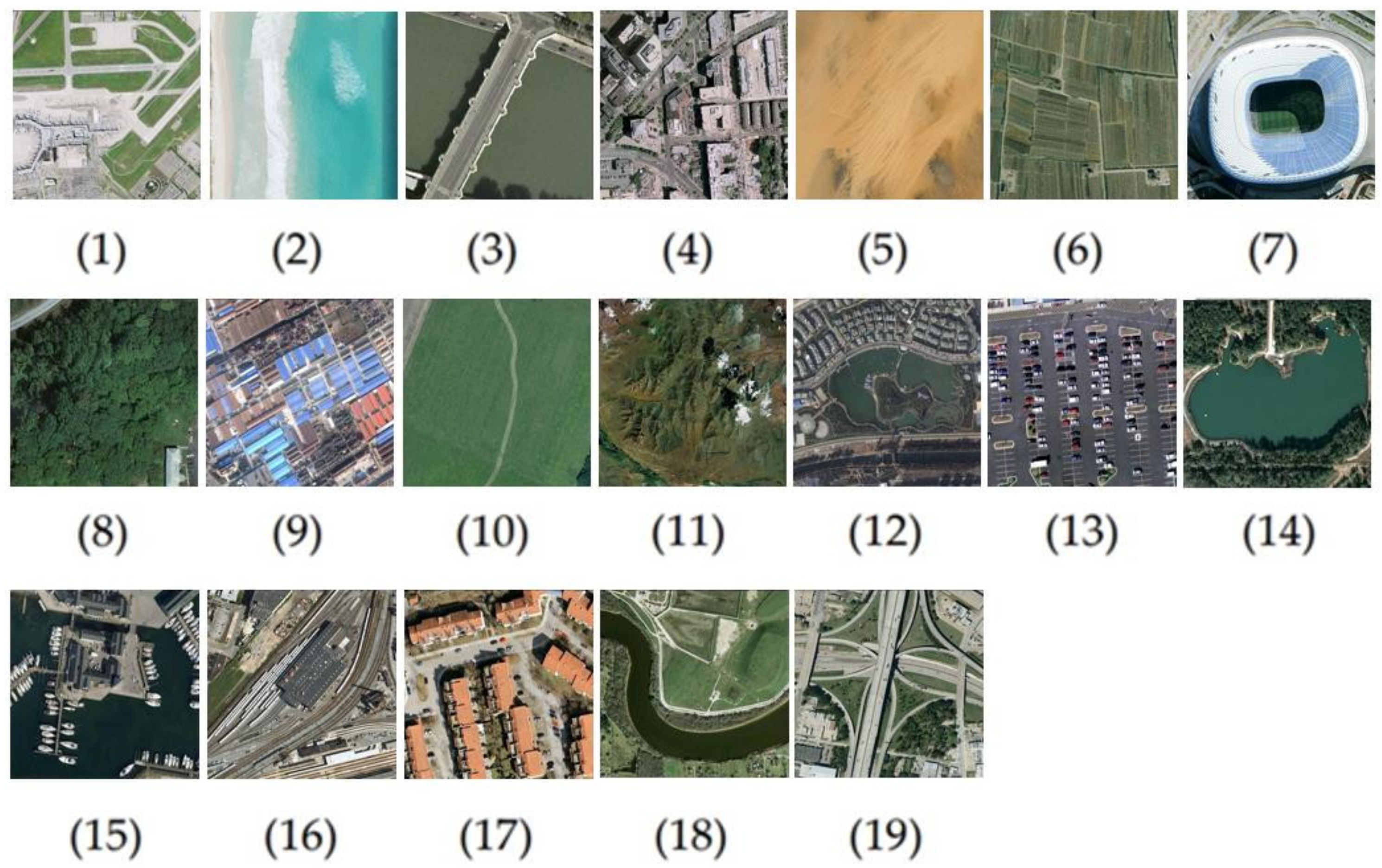
Applsci 11 11659 g001
Figure 2. Sample images of WHU-RS19 dataset: (1) airport, (2) beach, (3) bridge, (4) commercial area, (5) desert, (6) farmland, (7) football field, (8) forest, (9) industrial area, (10) meadow, (11) mountain, (12) park, (13) parking lot, (14) pond, (15) port, (16) railway station, (17) residential area, (18) river, and (19) viaduct.
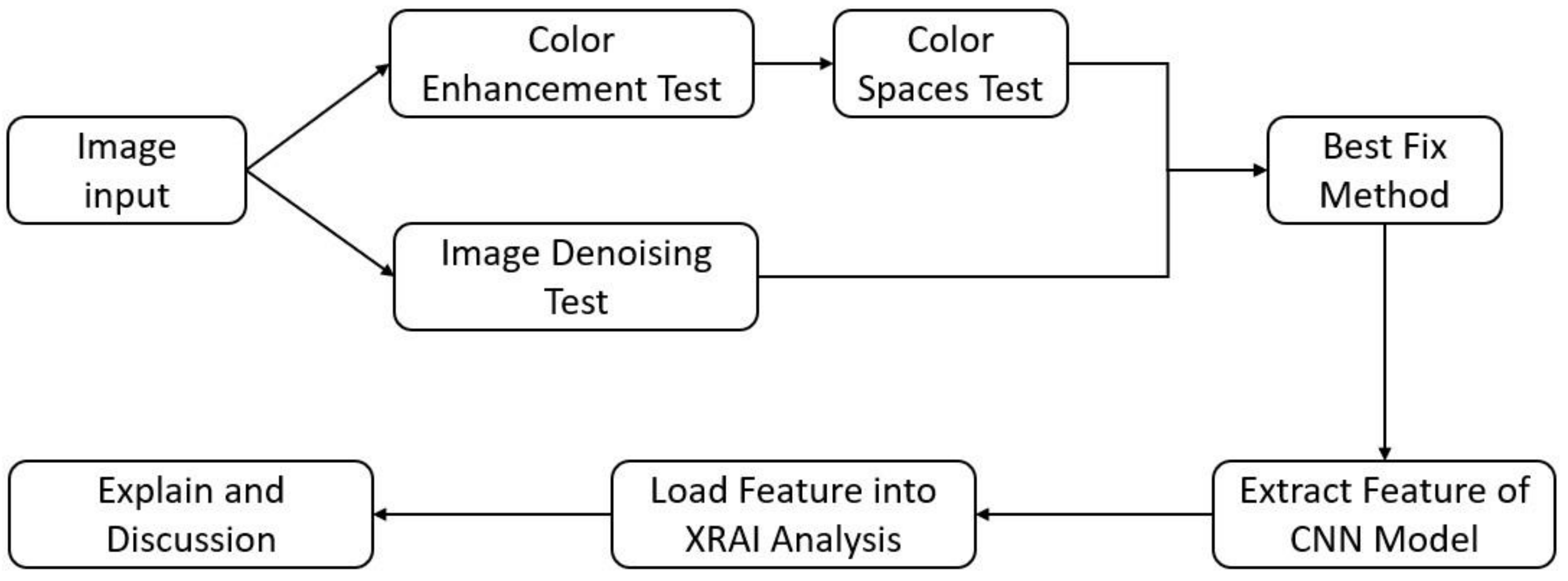
Applsci 11 11659 g002
Figure 3. Flowchart of the study design.
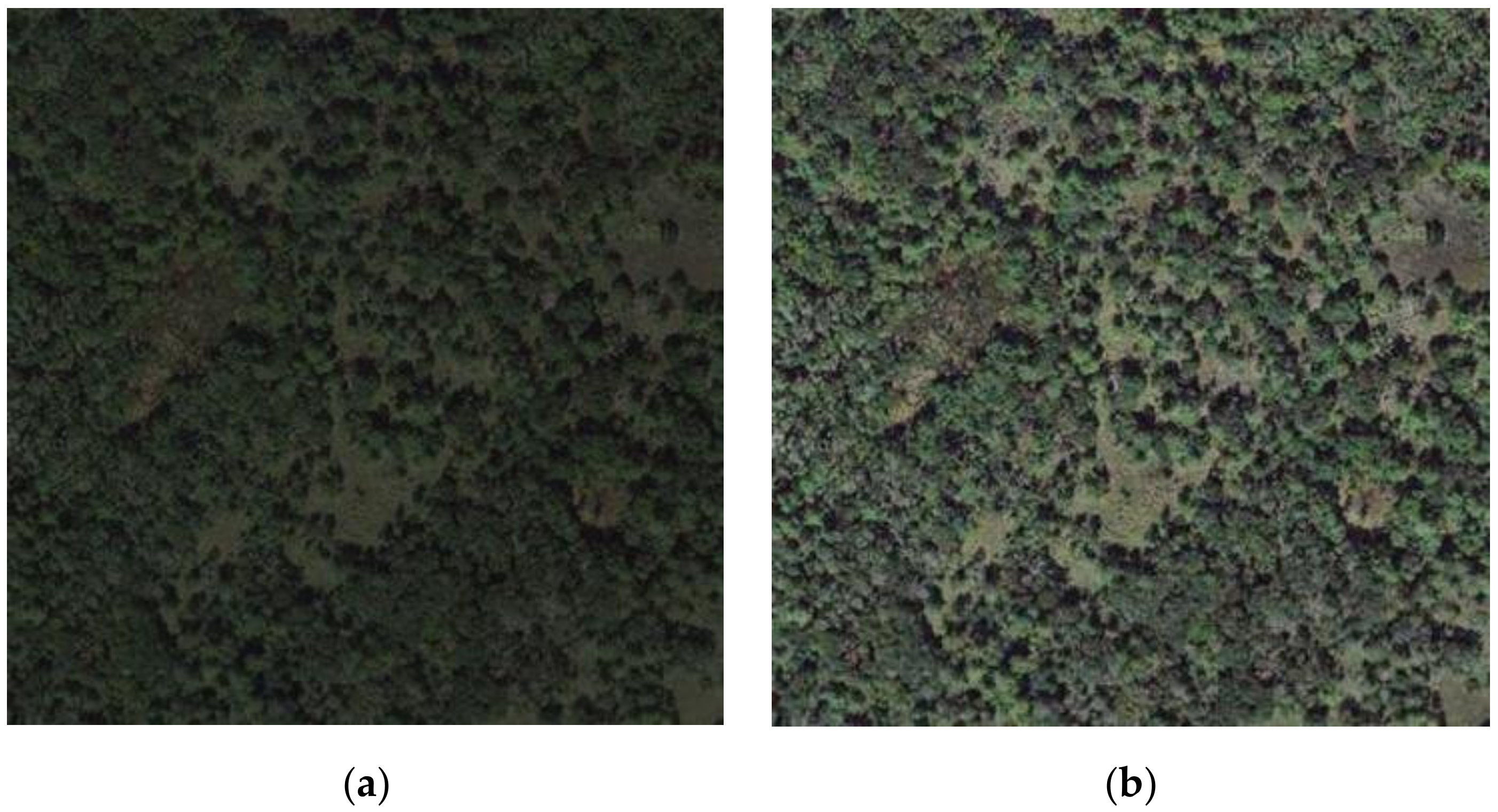
Applsci 11 11659 g003
Figure 4. (a) Original image. (b) Improved image using Gaussian Blur.
Applsci 11 11659 g004
Figure 5. (a) Original image. (b) Improved image using fastNlMeansDenoisingColored.
Applsci 11 11659 g005
Figure 6. (a) Original image. (b) Improved image using CLAHE.
Applsci 11 11659 g006
Figure 7. (a) Original image. (b) Improved image using MSRCR.
Applsci 11 11659 g007
Figure 8. (a) Original image. (b) XRAI shows the image feature hot zone.
Applsci 11 11659 g008
Figure 9. RSSCNet classifier network architecture.
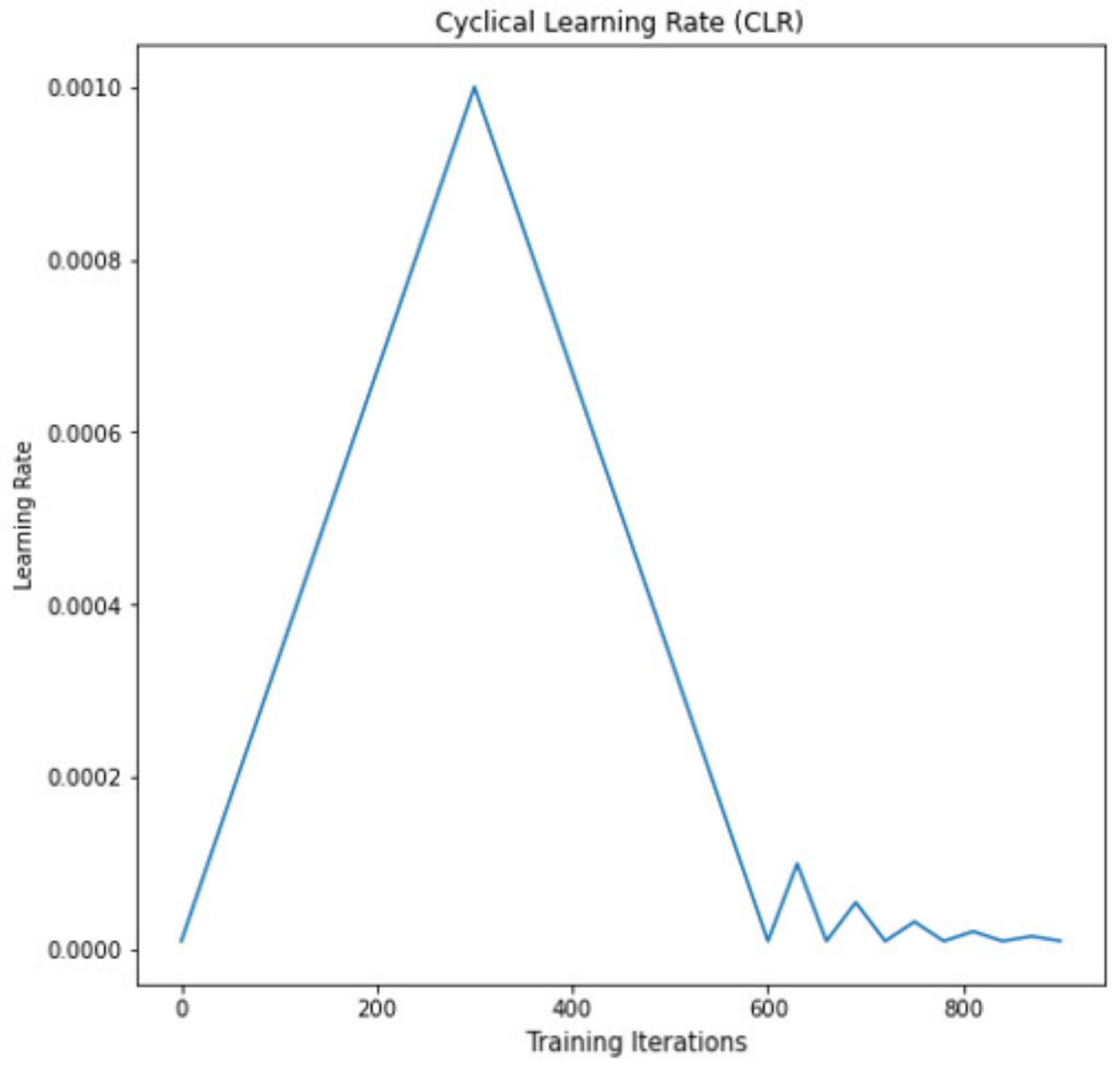
Applsci 11 11659 g009
Figure 10. Schematic of the two-stage cyclic learning rate training.
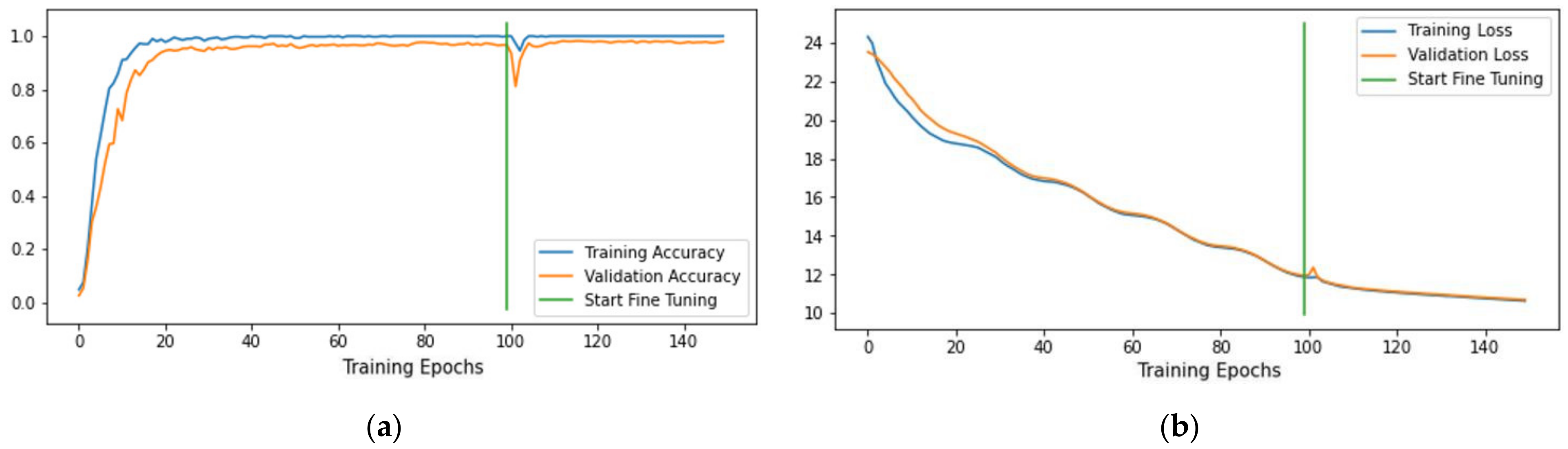
Applsci 11 11659 g010
Figure 11. Model training history of RSSCN7 dataset: (a) training and validation accuracy; (b) training and validation loss.
Applsci 11 11659 g011
Figure 12. Model training history of WHU-RS19 dataset: (a) training and validation accuracy; (b) training and validation loss.
Applsci 11 11659 g012
Figure 13. Image (river/lakes category) with XRAI analysis. (a) Original image (predicted as Industry); (b) improved image.
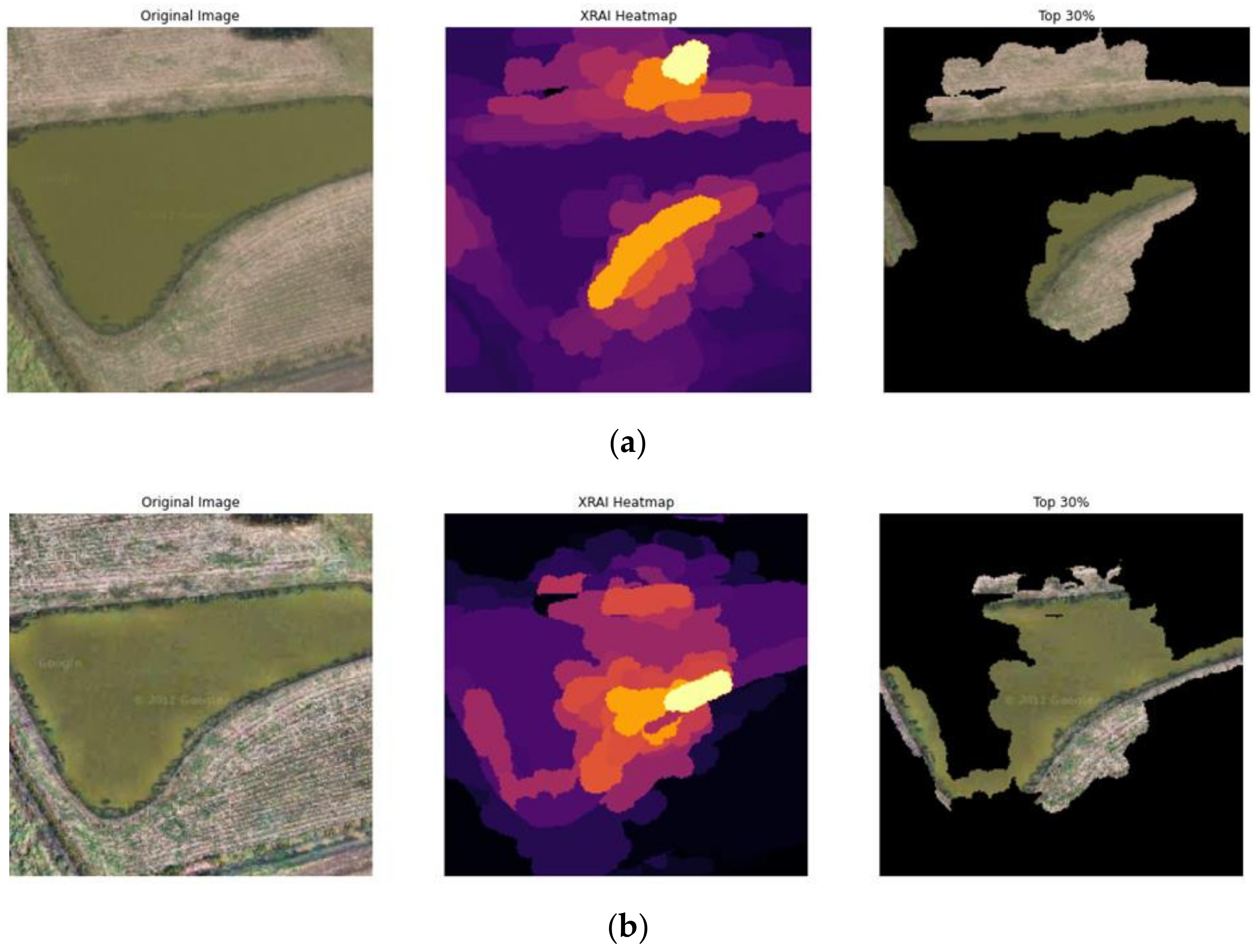
Applsci 11 11659 g013
Figure 14. Image (river/lakes category) with XRAI analysis. (a) Original image (predicted as field); (b) improved image.
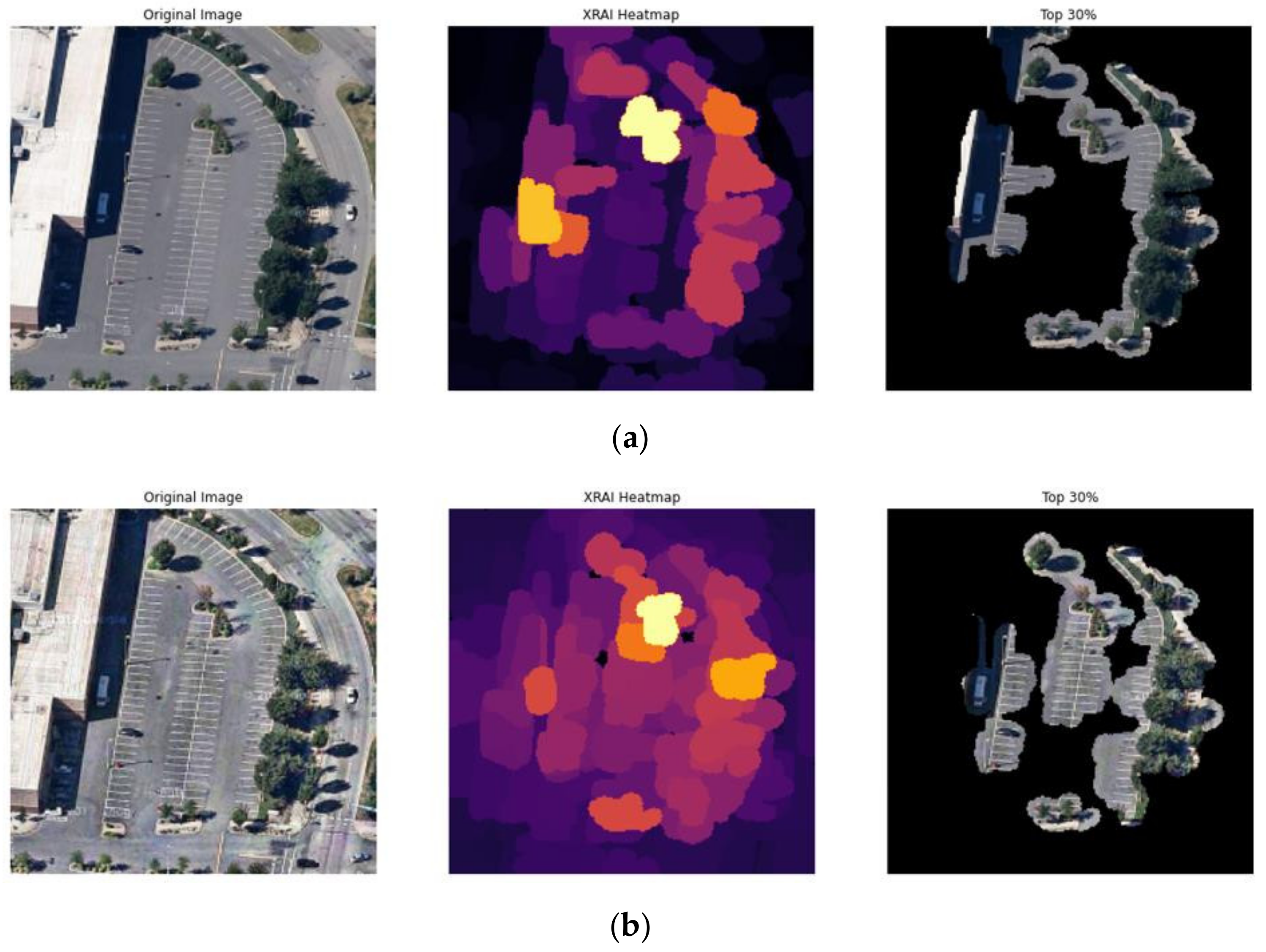
Applsci 11 11659 g014
Figure 15. Parking lot image with XRAI analysis. (a) Original image (predicted as industry); (b) improved image.
Applsci 11 11659 g015
Table 1. The main characteristics of the applied databases.
DatasetsImages per ClassClassesTotal ImagesImage SizesYear
RSSCN740072800400 × 4002015
WHU-RS19~50191005600 × 6002012
Table 2. Effect of image denoising methods on RSSCN7 dataset.
MethodTraining AccuracyTest AccuracyTest Correct Cases
Original Image1.00.95001330
Blur Sharpen1.00.95361335
Denoising1.00.94791327
Denoising Sharpen1.00.95861342
Blur Denoising Sharpen1.00.95501337
Table 3. Effect of image denoising methods on WHU-RS19 dataset.
MethodTraining AccuracyTest AccuracyTest Correct Cases
Original Image1.00.9768589
Blur Sharpen1.00.9768589
Denoising1.00.9768589
Denoising Sharpen1.00.9801591
Blur Denoising Sharpen1.00.9801591
Table 4. Effects of image enhancement methods on RSSCN7 dataset.
MethodTraining AccuracyTest AccuracyTest Correct Cases
Original Image1.00.95001330
CLAHE1.00.95861342
MSRCP1.00.94291320
Automated MSRCR1.00.95001330
Table 5. Effects of image enhancement methods on WHU-RS19 dataset.
MethodTraining AccuracyTest AccuracyTest Correct Cases
Original Image1.00.9768589
CLAHE1.00.9784590
MSRCP1.00.9619580
Automated MSRCR1.00.9635581
Table 6. Effects of color spaces on RSSCN7 dataset.
MethodTraining AccuracyTest AccuracyTest Correct Cases
Original Image1.00.95001330
RGB CLAHE1.00.95861342
LAB CLAHE1.00.95141332
HSV CLAHE1.00.95071331
Table 7. Effect of the proposed method on RSSCN7 dataset.
MethodTraining AccuracyTest AccuracyTest Correct Cases
Original Image1.00.9501330
Denoising Sharpen with CLAHE1.00.9651351
Table 8. Effect of the proposed method on WHU-RS19 dataset.
MethodTraining AccuracyTest AccuracyTest Correct Cases
Original Image1.00.9768589
Denoising Sharpen with CLAHE1.00.9801591
Table 9. Comparison of the overall accuracy on the RSSCN7 dataset.
MethodYearTraining Ratio
20%50%
DBN [10]2015NA77.00
GoogLeNet [20]201682.55 ± 1.1185.84 ± 0.92
CaffNet [20]201685.57 ± 0.9588.25 ± 0.62
VGG-16 [20]201683.98 ± 0.8787.18 ± 0.94
Deep Filter Banks [21]2016NA90.4 ± 0.6
GCFs+LOFs [22]201892.47 ± 0.2995.59 ± 0.49
RSSCNet [8]202093.51 ± 0.5197.41 ± 0.27
EfficientNetB3-Attn-2 [23]202193.30 ± 0.1996.17 ± 0.23
RSSCNet w/improved image (our)202193.76 ± 0.2597.94 ± 0.18
Table 10. Comparison of the overall accuracy on WHU-RS19 dataset.
MethodYearTraining Ratio
40%60%
GoogeNet [20]201593.12 ± 0.8294.71 ± 1.33
CaffNet [20]201695.11 ± 1.2096.24 ± 0.56
VGG-16 [20]201695.44 ± 0.6096.05 ± 0.91
TEX-Net-LF [24]201897.61 ± 0.3698.00 ± 0.52
Two-Stream Fusion [25]201998.23 ± 0.5698.92 ± 0.52
SE-MDPMNet [26]201998.46 ± 0.2198.97 ± 0.24
RSSCNet [8]202098.54 ± 0.3799.46 ± 0.21
EfficientNetB3-Attn-2 [23]202198.60 ± 0.4098.68 ± 0.93
RSSCNet w/improved image (our)202198.71 ± 0.2399.58 ± 0.07
Publisher’s Note: MDPI stays neutral with regard to jurisdictional claims in published maps and institutional affiliations.

