1. Introduction
Within the past decade, we could observe a massive increase in interest and results in the area of artificial intelligence. The market value of the field of artificial intelligence has grown drastically and is expected to be evergrowing. With that high interest and investments, not only have the possibilities of the artificial intelligence systems been enriched but their goals as well. More and more research conducted using artificial intelligence aims to solve more groundbreaking cases than categorising fishes to automate the sorting process. In previous years, we could observe a drastic increase in health-related or sustainability problems resolved using artificial intelligence [
1,
2,
3,
4,
5,
6,
7]. The development of artificial intelligence techniques leads to the development of the creators’ mindsets and their goals, increasing the want to analyse a tremendous amount of data to improve the lives of both people and our planet.
During the currently ongoing COVID-19 pandemic, we could observe how significant the delivery market is. Everyday transport of individual goods ordered online plays an essential part not only in our lives but in the increase of global warming as well. As the delivery routes consist of several scattered points with specific constraints, various possible paths exist that a delivery person can choose that day. Such a possibly trivial scenario is, in fact, an optimisation problem, dependent on various aspects such as weather and traffic conditions, the current state of the roadworks and others. An experienced driver will most likely be able to find at least a semi-optimal solution to this everyday problem, yet not always. As the driving conditions usually change faster than people habits, the better-known path might win over the slightly faster one. Even if that is not the case, humans cannot process the traffic data in real-time—contrary to computers. All those and many more aspects are even more important when it comes to inexperienced drivers. Helping them choose the best path is helping them to reduce fumes, emissions and traffic.
The increasing development of autonomous vehicles will most likely lead to a scenario where the packages will be delivered automatically, disregarding the human from the decision-making and planning process altogether. In this article, we try to deploy the reinforcement learning algorithms in order to test their suitability to optimise the route delivery vehicle—presumably a car—by learning algorithms to play a minimalistic simulation game focused on navigating through the grid-like map of a city while delivering packages from different locations scattered around the entire map. To best reflect the natural conditions, our simulation has selected fixed places with gas stations, while the collection and delivery of goods locations are random. During a single game, the agent’s task is to perform as many deliveries as possible while paying attention to the fuel level and available cash. The agent needs to learn when it is more profitable to drive to a gas station and when it is better to pick up a new task or end one already in progress. Additionally, the ever-changing environment and the continuous nature of the game require the agent to propose an initial solution and adjust and reevaluate every occurring change.
Due to that, this article attempts to find the most suitable method of taking those decisions among the two most developed reinforcement learning algorithms—Advantage Actor-Critic and Proximal Policy Optimisation with deeply learned policies [
8,
9,
10]. The deep reinforcement learning approach has been chosen even though classical search techniques usually work satisfactorily for such pathfinding tasks since the results achieved by those algorithms often surpass the expectations, finding more feasible solutions than those designed by humans. Additionally, the search algorithms require precise values corresponding to the paths, based on which they can evaluate different scenarios. As the data available for the agent in such a scenario would be distance, traffic, and others, rather than throughput time and gas usage—both of which would have to be estimated—graph-search solutions would require additional means of doing so. On the contrary, the reinforcement learning algorithms can learn to estimate those values exceptionally well—as part of their learning process—often surpassing humans’ possibilities and hard-coded algorithms, as was proven multiple times in the past [
11,
12,
13]. Deep Reinforcement Learning (DRL) has become a powerful and very popular tool recently. The first and most popular area where DRL algorithms are used are games. Algorithms based on DRL were proved to beat human players in such games like chess, Go, shogi [
11] or StarCraft II [
14]. Additionally, DRL algorithms have been successfully applied in recommender systems [
15], autonomous driving [
16], healthcare [
17], finance [
18], robotics [
19] and education [
20].
The most troubling aspect of reinforcement learning, which is the requirement for substantial quantities of the data [
8,
21], does not pose a problem in this scenario, as most of the delivery vehicles already have embedded GPS trackers. Thus, nearly every delivery company possesses real-life data about delivery targets and paths chosen by the drivers. Combined with the relatively accessible data (weather or roadblocks information), that can be utilised to construct an accurate model of the environment on which the agent can be trained.
In this paper, we are focusing on evaluating whether the two previously mentioned novel algorithms might be a suitable solution to continuous optimisation problems, even when the environment possesses a high degree of aliased states—states in which two or more different actions are evaluated as yielding similar rewards—which increase the complexity and uncertainty of the stochastic learning process.
2. Related Works
The topic of path optimisation using reinforcement learning algorithms has appeared in other publications as well. The reinforcement learning algorithms were recently used to path planning tasks for mobile robots. The most basic example is presented in [
22] where two algorithms, Q-Learning and Sarsa, were used to find the path between obstacles in a two-dimensional grid environment. Another approach to a similar problem was presented in [
23] where the Dyna-Q algorithm was tested in the warehouse environment. Not only table-based Q-learning algorithms were applied to solve the pathfinding problem in a grid environment, but also more complex approaches were tested. The Deep Q-Learning algorithm with convolutional layers is able to learn to find a path in small maps and also is shows promising results in finding paths on the maps never seen before [
24]. The Double Deep Q-Network algorithm was presented in [
25], where the agent had to learn how to find the path in the small environment (20 × 20 grid) with moving obstacles. In [
26] two deep reinforcement learning algorithms, namely Double Deep Q-Learning and Deep Deterministic Policy Gradient, were compared and was proved that the second algorithm gives better results in the task of path planning of mobile robots. Twin Delayed Deep Deterministic policy gradient algorithm combined with traditional global path planning algorithm Probabilistic Roadmap (PRM) was used for the task of mobile robot path planning in the indoor environments [
27]. The presented results indicate that the generalisation of the model can be improved using a combination of those methods.
Another example of similar work is the usage of Deep Q Learning combined with convolutional neural networks in order to develop a path planning algorithm for a multiagent problem, proving that such algorithm can produce an effective and flexible model performing well compared with existing solutions [
28]. Other scenarios where reinforcement learning algorithms were also utilised is the optimisation of the paths for marine vehicles [
29,
30]. Furthermore, the Q-Learning approach was utilised in order to create a navigation model for smart cargo ships [
31]. The authors proved that the approach proposed in the paper is more effective in self-learning and continuous optimisation than the existing methods. Another example of using DRL algorithms for the task of path planning for crewless ships was presented in [
32]. The authors used the Deep Deterministic Policy Gradient algorithm to learn the agent optimal path planning strategy. Further, the original DDPG algorithm was improved by combining it with the artificial potential field.
A new reinforcement learning algorithm, named Geometric Reinforcement Learning, was derived and proposed in order to improve the pathfinding process of Unmanned Aerial Vehicles [
33]. Duelling Double Deep Q-Networks were used in order to achieve real-time path planning for crewless aerial vehicles in unknown environments [
34].
Another area of research where DRL algorithms were applied is the problem of area coverage. Optimising the coverage path planning is essential for cleaning robots, which are now very popular [
35]. The Actor-Critic algorithm based on a convolutional neural network with a long short term memory layer was proved to generate a path with a minimised cost at a lesser time than the genetic algorithms or ant colony optimisation approach [
36]. The recurrent neural network with long short term memory layers using DRL was proposed to solve the coverage path planning problem in [
37]. This method was shown to be scalable to the larger grid maps and outperforms other conventional methods in terms of path planning, execution time and overlapping rate. Deep Q-Learning and Double Deep Q-Learning algorithms were applied to solve the patrolling problem for autonomous surface vehicles [
38]. The proposed approach was compared, and proven better, with three different algorithms: a naive random exploration, a lawnmower complete coverage path and Policy Gradient Reinforcement Learning.
The literature review showed that the reinforcement learning algorithms performed well for pathfinding and area coverage tasks. That is why we decided to check their effectiveness in the case of a more complex problem, which is not only determining the path between points but also deciding when it is more profitable to start a new task or refuel the vehicle. In the proposed scenario, the agent has to learn not only the optimal path between two points but also whether it is better to go for the new task or to go to the station and refuel. The decision has to be made taking under consideration the closeness of the stations, amount of available money and distance to the following quest points. Because the only constant element of the considered map is the station’s position, the problem to solve becomes even more complex. Additionally, the aforementioned solutions use much less advanced algorithms compared to this paper, in which we evaluate the two of most novel approaches—Advantage Actor-Critic and Proximal Policy Optimisation. Those techniques promise enhanced results yet cost additional complexity—thus, investigating their applicability to this particular scenario is vital, as this trade-off might not be beneficial; this paper proves otherwise.
3. Materials and Methods
3.1. Motivations for the Reinforcement Learning Approach
Ever since the groundbreaking publication about mastering Atari video games with reinforcement learning algorithms [
39], this previously almost forsaken pillar of artificial intelligence began to gain more and more popularity. Even though it is far from the popularity of supervised learning, not only the number of problems solved with reinforcement learning but the diversity of their areas has increased as well. While remaining probably the best approach towards learning agents to play video games, reinforcement learning has proven to be extremely effective in other cases, such as traffic control [
40], robot controlling [
41] or cancer treatment [
42]. Since the learning process is based on the rating of the results rather than the decision-making process, this approach works exquisitely with complex or even impossible problems for humans to evaluate; such as being hardly solvable with supervised learning algorithms or due to having costly or impossible to label data. This scenario is more widespread than might be anticipated, as it occurs in many problems that are different from classification. It is tough to say with 100% certainty which action or decision is ultimately best in a particular situation in various scenarios, such as a game of chess. What is more, the process of translating human knowledge into a form suitable for computers is often imperfect in less straightforward scenarios. Even chess masters cannot formulate the calculations driving their movements in the form of precise numbers or equations that might be utilised as input for graph search algorithms. Thus, it is often more efficient to let the machines learn those values by themselves—with reinforcement learning algorithms—than trying to enforce possibly imperfect and definitely loosely translated human knowledge.
On the other hand, such a process of almost complete self-learning comes with its price, as it requires not only a significant amount of time but numerous data samples as well. Without anyone pointing the algorithm in the direction of the solution, the reinforcement learning agent has to discover everything on its own while interacting with a computer model, representing an abstraction of a problem—usually referred to as the environment. The design of that model is fundamental in the learning process, as the entirety of the agent knowledge is derived from the interaction with it. To be accurate in representing the actual scenario, this model has to be well-designed based on the numerous data samples describing the problem.
Additionally, as mentioned before, the significantly higher learning time—compared with the supervised learning approach—is another important drawback of reinforcement learning. This problem is partially mitigated with new approaches such as Asynchronous Actor-Critic and due to vast improvements in the area of graphic card computing power and its applicability in deep learning, yet it still remains an issue.
Considering those possible gains and the drawbacks in this article, the applicability of the reinforcement learning approaches in the scenario of path-planning for deliveries is tested. For that purpose, the two most prominent reinforcement learning algorithms were chosen—the well-known and widely considered as state-of-the-art Advantage Actor-Critic (A2C) approach with and without novel improvement in the learning process, known under the name of Proximal Policy Optimisation (PPO), implemented and learned over a custom-made grid-like environment. As mentioned previously, both of those algorithms can be considered state of the art, as they are two of the most complex and novel out of critically acclaimed reinforcement learning algorithms. The results of those learning processes and conclusions and possible developments are discussed later in the article.
3.2. Advantage Actor-Critic and Proximal Policy Optimisation
The Actor-Critic is a family of three similar yet somehow distinctive approaches, considered currently to be the most effective reinforcement learning approaches [
8,
10,
43]. Those are Actor-Critic (AC), Advantage Actor-Critic (A2C) and Asynchronous Advantage Actor-Critic (A3C). The names are derived from the fact that the agent consists of two value functions, one designed to evaluate the policy and the other for grading the partaken actions. Such separation of the functionality allows the agent to learn stochastic policies, which tends to work better than the deterministic value-based approach [
8,
43].
While actor function learns how to act in the environment, the critic learns to evaluate their actions. They both support each other in their learning processes, as improvements of the critic lead to better decision making, which leads to the discovery of new states as situations not known previously to the critics, thus improving his perception and evaluation. To improve that process even further, the Advantage Actor-Critic approach learns the actor by evaluating the advantages—changes of “quality” of state transformation—rather than the actions themselves. This increases the stability of the learning by the introduction of a baseline and simplifying the working principle of critic from the evaluation of the actions with respect to the state into the evaluation of the state itself. Lastly, the A3C approach improves the data gathering with asynchronicity—while the actor and critic are learned, the data is gathered with the usage of old parameters, which are updated periodically. This increases the speed, especially in the scenarios in which the data gathering process is time-consuming yet might hinder the process, as the actor is acting based on the outdated parameters most of the time.
The A2C approach was chosen over the A3C (Asynchronous Advantage Actor-Critic) since the main improvements provided by the A3C revolve around increasing the speed and efficiency of data gathering, which was not a problem in this particular scenario, and the possible drawbacks might overthrow the gains.
The formula for the parameters update is described by Equation (
1) [
8,
10,
44]:
where:
and:
—parameters of the policy network,
—actor learning rate,
—gradient with respect to the parameters,
—probability of taking action a in state according to the current policy ,
—value of a state S at time t,
—estimated advantage at time t.
The actor uses gradient ascent in order to minimise the inverse of the reward function—hence making the designed positively rewarded actions more probable. To ensure that the learning process is robust versus the possible randomness of the rewards, the value function’s yield is multiplied by the probability of taking such an action. If the action is considered to be impaired by the actor—and thus, has a small probability of being chosen—the loss is significantly decreased in order to ensure that the step taken in this unlikely direction is cautious. If, however, the action turns out to be desired, with the increase of certainty for choosing this action, the update step increases as well. That formula ensures that even if a destructive action yields good results—due to sheer luck or as a result of previously taken actions, for example—it will not destabilise the learning process as much as it might.
On the other hand, the critic learning process usually follows the temporal difference algorithms. The formula for step update is presented by Equation (
3):
where:
—value of a state S at time t,
—reward obtained from transforming between states and ,
—actor learning rate,
—discount factor.
Equation (
3) [
8,
45,
46,
47] describes one of the first widely used reinforcement learning algorithm. It is still commonly used as one of the most reasonable ways of learning value-based estimators to solve more straightforward or particular problems or as the critic part of the Actor-Critic algorithms [
8,
10,
44]. The update is based on the estimation of this and consecutive state—both of them utterly wrong at the very beginning of the learning—with the one fundamental element—reward generated by the actions. Since the values provided by the value function represent the estimation of all the rewards that are obtainable from this particular state, the values of two consecutive states should differ only by the value of reward generated during the transition. Updating the parameters so that the obtained difference is closer to the actual reward allows the critic to learn how to predict those values precisely. Since both the previous and following state values have to be estimated, the constant shift of the parameters affects not only the estimations but the learning targets as well. This affects the learning in an undesired way and has led to the approach referred to as target critic networks—using slightly outdated parameters for estimating the learning targets and updating them periodically to stabilise the learning process. As the targets become fixed for a period of time, the value function can tune its parameters to resemble expected outputs rather than shift chaotically with every update. This particular approach is widespread and extremely effective [
48,
49]; hence it should not be surprising that a somewhat similar technique has been adapted to the actor learning process under the name of Proximal Policy Optimisation.
The main concepts of the PPO remain the same—stabilise the learning in order to increase its efficiency. However, it is driven by a slightly different mechanism—clipping the learning loss to reduce the variance. The clipping equation is presented in the Equation (
4) [
9,
50].
where:
—ratio between the probabilities calculated with current and old parameters,
—estimated advantage at time t,
—clip ratio.
In Equation (
4), the probability of performing the action has been replaced by the ratio between probability under current vs. previous (target) parameters. Even though this increase the absolute value of the losses—as the ratio much often takes higher values (close to 1) than the probability of performing a particular action—this approach decreases the possible variance between the losses. As mentioned previously, the optimisation step’s size increases with an agent’s increasing belief in action. This can lead to a situation when upon discovery, a new action becomes mistaken for a lucrative and a cycle of exploitation; this possibility creates an avalanche-like process of a massive shift in parameters towards this action, as with every learning iteration, the losses increase drastically. PPO prevents such a situation by ensuring that the loss correlated with agents predictions can only grow as much as the
parameter allows during a short period of time [
9]. Due to that, minor variances causing the agent to look more optimistically at some actions do not destabilise the learning as much as they possibly would, thus usually increasing the stability of the entire process [
51].
Deep Learning
Both implementations of the algorithms used in this paper are utilising the deep neural network as functions approximators. The Actor-Critic methods utilise two function approximators; therefore, there exist two solutions for that situation—a classic single-headed neural network for each of the modules, or more novel, a single two-headed neural network in which actor parameters are more imperative. The latter promises a faster learning process due to the smaller number of parameters, and thus, a lesser amount of computation is required with the learning cycle, yet they couple the critic and actor results together, making them partially dependent [
10]. Due to that, in this article, the classical single-headed approach is used. The parameters used for the neural networks are presented in
Table 1. Both of the networks are visualised in
Figure 1.
In both of the implementations, the neural networks used for the function evaluations consisted of two hidden layers. The first is of significant size to ensure that the number of parameters for processing the above-average large-state vector would be sufficient. The second hidden layer has different sizes for actor and critic networks due to the linear activation of critics output, which usually works better with a smaller number of parameters due to fewer variations. However, the main difference between the actor and critic is utilising the LeakyReLU instead of a ReLU activation function in actor networks. In the actor’s case, the LeakyReLU was more suitable since due to negative reinforcements of some actions, the negative values are more likely to occur, while most of the critic values are somewhat positive due to the minor death penalty. Nevertheless, both of those are commonly used in deep reinforcement learning [
52,
53]. The actor’s output layer is utilising Softmax activation in order to provide the outputs in the form of a stochastic probability distribution rather than a deterministic decision.
The networks and their gradients were implemented and calculated with the usage of the PyTorch library, as its functionality suited better the reinforcement learning approach. The ability to manipulate the losses before the backpropagation aligned with the gradient descent of the Advantage Actor-Critic optimisation step (Equation (
1)) in which the loss from the policy is multiplied by the expected advantage provided by the Critic network. The optimiser chosen for both networks is Adam, which, due to its robustness, is one of the most commonly used optimisers.
As powerful as it is, deep learning comes with some drawbacks. Most importantly, in terms of reinforcement learning, the data’s high sequentiality impedes the learning process drastically. Since the data used in reinforcement learning are strictly sequential—one state derives from another with minor changes—additional measures have to be implemented. To cope with that, the idea of replay memory has been introduced [
54,
55,
56,
57]. Instead of instantly analysing the samples, every action is recorded and stored in the memory buffer, from which randomly shuffled batches of samples are retrieved whenever the learning takes place. Those buffers can be implemented under two systems—prioritised and unprioritised. The latter samples every sample with equal probability, while the first does not. Usually, the priority of sampling is correlated with the reward obtained during that sample or loss generated while analysing this sample. In this article, the first approach was chosen—the actions yielding rewards were stored in a separate buffer and sampled with higher priority. To counter the fact that high reward actions could be possibly displayed multiple times, their losses were additionally decreased by a hyperparameter referred to usually as ISWeight—0.03 in this case. Due to that, high impact actions were often partaking in the learning process, yet their impact on the parameters was decreased to ensure slow but steady progress in their direction.
3.3. The Environment
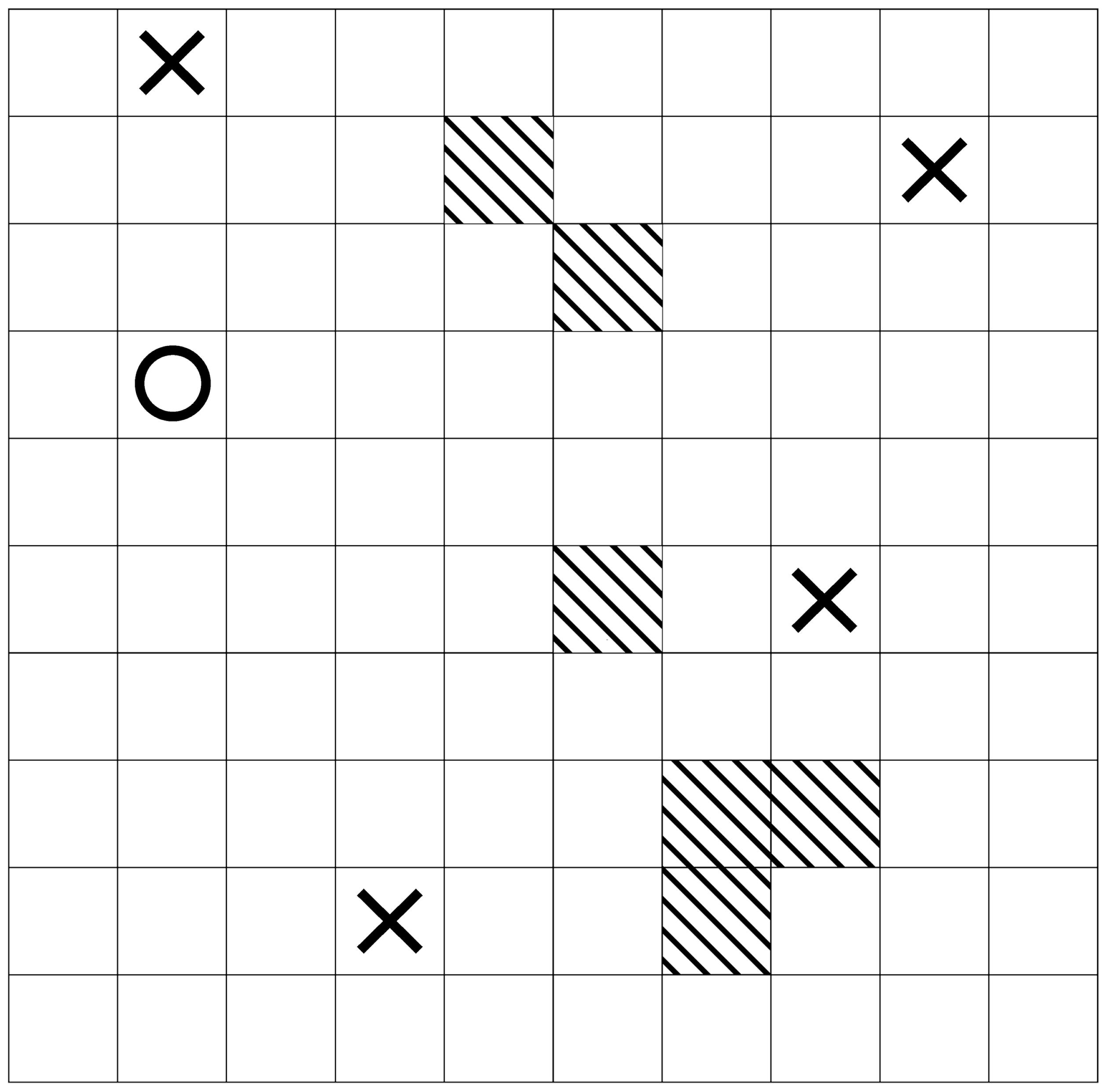
The data used in the learning process were obtained from the agent’s interaction with the environment—an abstracted representation of the actual scenario, feasible for the automatic processing, provided in the form of a game. The design and implementation of the environment play a crucial role in the reinforcement learning process, as the agent’s complete knowledge is derived from the interaction with it. Therefore, it is essential to abstract the problem without losing the parameters that are vital for the decision process.
In this case, the delivery area map was abstracted into the form of a grid to form computationally feasible data (
Figure 2). Such an approach has been previously used and tested in reinforcement learning scenarios with satisfactory results [
8,
58,
59,
60].
The environment map consists of a 10 × 10 grid, with 10 objects of interest—6 fixed gas stations and 4 quest instances scattered through the map. The quest instances are generated randomly—at the beginning of every episode and upon interacting with one of them. Since only four can exist simultaneously, the next is spawned instantly upon completion of one of them. To complete the quest, the “package” has to be firstly retrieved from a quest location. Upon that, the random reward location with the corresponding monetary reward is generated—the further the destination point, the higher the “in-game” reward for completing that task. To make the learning process slightly more manageable, the quest’s initiation provides the agent with a small reward—10% of the total reward (meaning both the reinforcement learning reward signal used in the learning process and in-game monetary reward) as a form of an advance, deducted from the total reward received at the end. This applied to the money obtained for completing the quest as well. The agent could later use this money to fill the gas tank while visiting the tiles containing the gas station to prevent his death. The maximum and start capacity of the gas tank was set to 30—forcing the agent to incorporate tanking into the plan quite often. Additionally, this action is not available to the agent at the very beginning of the episode, as initial funds (required to purchase the gasoline) are set to 0. In order to earn the required money, the agent has to begin or complete a task first. To achieve a smaller variation of the learning process, the magnitude of the rewards received by the agent was pretty small. For completion of the entire quest, the agent would receive a positive reward of size 1 (10% of which at the beginning) and −0.1 while losing due to the empty gas tank. Such design of the environment allows us to ensure a sufficient level of complexity, as randomisation of the reward location generation and the fact that there can be multiple quest objects at once (each of them with a different reward for completion) requires the agent to constantly take multiple factors into consideration and forces it to reevaluate the plan on every quest completion, as the new locations cannot be predicted and planned earlier.
The state vector provided by the environment is presented in
Figure 3. To ensure that the agent possesses all the necessary information required for the learning process, the entire “map” of the game environment is represented as the vector of size 100 (
Figure 3—
I), where particular cells correspond to map tiles. Tiles values are set to 0 if empty; Otherwise, distinctive values based on the object inside—255 for the player, 140 for the reward location, 100 for a quest location, and 50 for a gas station. After that, the percentage of the gas tank is appended (
Figure 3—
II). The last feature describes the amount of money available for the agent. The amount of the available money is divided by 500 and then clipped to the interval <0, 1> and stacked at the end of the feature vector (
Figure 3—
III). This state representation might be treated as suboptimal since the input vector is quite long for such a simple scenario and might significantly increase the learning time, yet it allows the agent to grasp the complete picture of the situation. A possible alternative to such a scenario is utilising convolutional neural networks, proven to handle the game environments well. However, in this case, the map is fairly simple, and adding a graphical layer to the learning process would most likely provide more overhead than benefits, given relatively short learning time.
3.4. Learning Hyperparameters
The hyperparameters used during the learning process are presented in
Table 2. This time, the differences between the A2C and PPO implementations are more visible. As mentioned previously, the increase of the loss values caused by switching from probabilities (which oscillates around 0.25–0.6 most of the time) to the ratio (oscillating around 1) is countered by decreasing the learning rate of the actor. On the other hand, the critic’s learning rate has been increased, based on the previous iteration observations. Both of the implementations use exactly the same memory system—the memory is divided into two subsets—priority buffer, storing the samples with non-zero rewards, and regular memory buffer, storying memory chunks that yielded no rewards. That implementation might come as unusual, as classically, the prioritised buffers are implemented in the form of SumTree [
57,
61,
62], allowing for statistically correct retrieval based on the priorities. However, such implementation causes come with the drawback of significant computational overload connected with the need for restructuring the tree with every added sample. Since the number of average samples per iteration is relatively high—compared to the 38 moves per chess game [
63], for example—and the importance of a single sample is much more minor, such an overload was not compensated with the benefits of statistically meaningful prioritisation of the memory. Instead, the samples of fixed sizes (
Table 2) were taken from both of the buffers and shuffled (in order to avoid drawbacks of sequentiality). Since the fixed number of high reward samples might disrupt the learning process providing constantly high loss values, the loss obtained from the high priority samples was decreased in magnitude by a constant factor (
Table 2). The target network was updated and at the same pace as the parameters of the “old” agent used in the clip ratio calculations (Equation (
4)). The clip value was chosen to be 0.2, as recommended in the initial PPO article and other publications [
9,
50]. Lastly, it is essential to note the lack of any parameters connected with the exploration. The environment’s mechanics are straightforward and do not require any complicated sets of actions to be discovered; thus, no additional exploration mechanism is implemented. The entire exploration mechanism is based on the stochastic policy, which allows taking other actions than currently evaluated as best, hence satisfying the need for exploration [
8].
4. Results
Finally, the algorithms were trained for ∼1,500,000 iterations in the case of A2C (∼48,000,000 chunks of experience) and ∼1,000,000 iteration (∼32,000,000 chunks of memory analysed) in the case of PPO. During the learning process, the various data regarding learning and performance was observed and stored to visualise the progress. The following section is divided into two parts. First, the description of the observations gathered during the learning process—which is a vital part of the evaluation of applicability, as they present some level of abstraction from a particular implementation of the environment; observing the trends in the learning process, we can draw some additional conclusions on what the performance could be, given sufficient learning time. Secondly, we test the performance of learned agents over several iterations and present the results in the table to allow comparison between the two selected algorithms.
4.1. Learning Process
The following section summarises the observations gathered during the learning process of the algorithms. It describes the performance as well as other factors vital to the learning process, such as loss values or certainty with which the policy was taken. All graphs presented below are smoothed using the sliding window technique in order to ensure proper visualisation of the trends and clarity of presented data.
4.1.1. A2C
As an initial implementation, the A2C implementation was trained significantly longer to ensure its progress. The final results of that are presented below, in
Figure 4. In order to achieve readability in
Figure 4, each point of the line is created by averaging using the sliding windows technique—taking an average from multiple points behind and after the current one. In that figure, as well as in all of the figures from the A2C section, the window size is set to 10,000, meaning that each point is an average from 5000 previous and 5000 next episodes.
Performance
The first interesting take-away from the graph is the fact that the first 10,000 episodes performed outstandingly well compared to the numerous episodes ahead. This is the result of PyTorch model construction, which initialises new models in such a fashion that regardless of the inputs, the outputs tend to be almost identical, creating a nearly uniform random exploration policy at the very beginning of learning. As the parameters get slightly pushed into the direction of any action, the performance drops drastically, as the random exploration gets reduced to the part of the map, to which leads the most probable action currently; thus reducing the number of fields that are likely to be visited from the entire map, to some part of the map towards the preferred direction. This creates the illusion of errors in the learning process; however, it is just a misunderstanding, as the initial performance was not good at all; it just could lead to decent results due to environment mechanics and luck.
Despite the initial drop of the score, the graph clearly represents the mountain climbing process—small yet persistent steps toward better results and self-improvement. There are visible up and downs, especially in the middle part of the training. However, the trend is persistently increasing. Such behaviour is very much expected when it comes to reinforcement learning, which often requires some significant amount of time to achieve even decent results.
Another set of data gathered during the experiment is the total loss of the batch sampled for the learning process, both for critic and actor. As can be clearly seen in
Figure 5a,b, curves presented by those do not differ much. However, it is important to recognise that those similar curves represent different behaviour. The decrease of the critic losses means approaching the optimum—the initially random policy is performing better and better at guessing the rewards yielded from state transformations. On the other hand, when looking at the actor loss curve (
Figure 5b) it is worth noting that the slope’s direction is negative, as the actor losses’ values have a slightly different meaning than usual. Instead of quantity measuring the distance between correct and predicted values—which cannot be negative—the losses are used to measure an actor’s performance. They can be either negative—if the action is rated as inferior—or positive—if the action is favourable (Equation (
1)). However, since the deep learning libraries provide the utilities to perform a gradient descent, the sign of the losses has to be flipped to retain the desired direction of the optimisation step. In this particular case, the sum of the losses is always negative—meaning that there were more positively rated actions in the batch than not. The reason for that lies in the environment’s design—the negative signal is much smaller and appears only once, while there are more possibilities—in fact, infinite—for actions resulting in the positive signal during one episode. Thus, much more actions would yield positive than negative signals, causing the algorithm to reinforce action more often than not. The one important note about this graph is the fact that the curve is still clearly increasing. It is somewhat not flattening yet, and it might even accelerate. This shows that the actor parameters are still far from the convergence—even after 1,000,000 learning episodes. This could be expected, as the number of iterations used to train this algorithm is relatively small, compared to other studies [
64,
65]. In fact, achieving effective policy seems to be only started, and much more computing time and power have to be used to achieve perfection.
Movement during the Learning Process
To allow for a deeper look into the learning process, additional data about an agent’s behaviour during the learning was recorded. These parameters are the mean certainty of taken actions during the episode and the percentage of “invalid actions”—the attempts to exceed the map’s boundaries.
The two final
Figure 6a,b visualise the mean probability of the actions chosen during the iteration and the percentage of invalid movements—those which try to exceed the boundaries of the map—accordingly. As is visible in
Figure 6a, the actions’ probability is rising drastically fast—starting at almost 50%. It is worth noting that due to the policy’s stochasticity, the highest values of a probability are tough to achieve, as the actions with minimal probability still can be selected, significantly reducing the mean. After that initial rise, the certainty spikes to almost maximum. This is the previously mentioned part of the graph, which yielded inferior quality of performance at all fronts—low rewards and steps and a high degree of invalid movements. That, however, does not last long and quickly transforms into the next part of the learning, with remarkable high variance (visible as a thicker line in
Figure 6a—it is a highly variated line going up and down constantly). The reason behind such variance in this particular part of the learning remains unknown; it is, however, evident and thus worth noting. The last part of the graph represents the stable and persistent progress achieved after some initial setbacks in the same fashion as all other parameters. The sudden drop in certainty might seem like a step backwards; however, it represents the next level of awareness in the case of planning. In fact, various quests can be ended by following different paths, and the availability of multiple quest points allows one to focus not only on one, decreasing the certainty over one specific path and allowing for other movements. Instead of blindly following the directions which were considered best, agent actions became more situation-dependent and agile, which is a crucial concept in planning strategy in such environments. The last figure,
Figure 6b, represents the percentage of invalid moves. The initial high value in the early stages is caused by too much certainty. After that, a slight but steady decrease toward optimal value can be observed. It is worth noting how high the final value of invalid movements is. Even after so many episodes, around 4% of the agent’s actions—some of which might be random—do not affect the environment.
4.1.2. PPO
The learning process of the agent with the usage of PPO was significantly shorter. However, it can be observed that the results are much more promising. The following subsections present those results and highlight the most important differences. Same as in the previous section, the graphs presented here are smoothed with the usage of the sliding window technique to ensure readability.
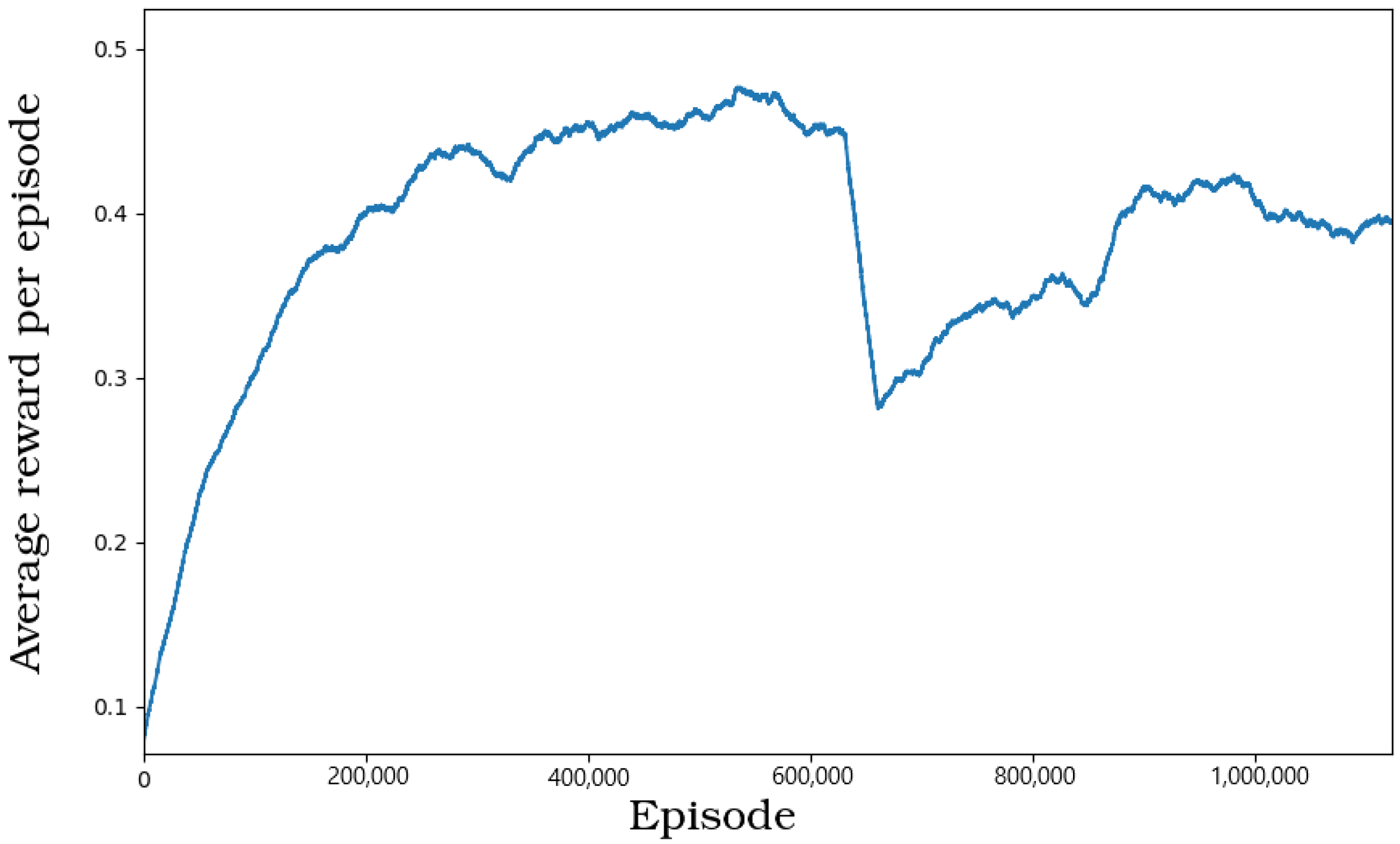
Performance
Figure 7 presents the reward values obtained during the PPO learning process. The first noticeable thing is the high spike right in the middle of the graph. A remarkable shift in most of the other learning parameters is noticeable around the same iteration, most due to exploding gradients, as both critic and actor present some drastic variations at that moment. Apart from that one shift in the performance, the graph’s curve clearly shows another hill-climbing process—slowly yet steadily increasing the performance over time. Even after that sudden and abrupt drop, the agent is slowly coming back to his previous performance. Compared to the reward curve of A2C (
Figure 4), this process is much faster and characterised by smaller variations. The final values obtained by the actor are higher than the ones from A2C implementation, despite the fact that the agent was trained less.
The graphs (
Figure 8a,b shows the values of the losses used for learning through the entire process. From the very first glance, it is visible how different they are from their counterparts (
Figure 5a,b). The reason for that lies in as the priority memory buffer implementation guarantees that two high-value chunks—which are much more likely to generate high loss values—will be present in the learning batch. Due to that, dozens of very steep up-and-down movements are visible. Since the high-value samples could be completing a quest (0.9), starting a quest (0.1) and losing (−0.1), the uneven distribution of those causes formulation of such spikes on the graph; since with the priority batch of size two an even distribution is impossible to be achieved, such situation repeats itself a few times during the learning. It appears to give much higher variation in the PPO implementation; this is caused by the fact that absolute values of the critic losses are around four times smaller—and thus, they appear bigger. This could be prevented with the usage of a more sophisticated memory buffer and sampling method, yet the computational cost required to form and expand such data structure would cause more pain than gain. On the other hand,
Figure 8b is characterised by the same spike in the middle, visible previously in
Figure 7. As the performance of the actor dropped, the high reward samples became less likely to appear in the priority buffer, thus reducing the total loss values.
Movement during the Learning Process
As in the previous case, the data about the agent’s behaviour during the learning process was gathered.
The last two figures,
Figure 9a,b, visibly differ from their counterparts (
Figure 6a,b). The certainty, as previously, starts around 50%, yet it decreases rather than increases during the learning. This does not necessarily mean that the actor performs worse—as there always exist multiple viable paths, decreased certainty shows the increased level of spatial awareness of the actor, who can see the resemblance between paths and juggle between them, rather than follow a path from memory. Keeping the probabilities smaller than 50%, yet presenting the increasing trend, shows that the agent learning process is more optimal than before. Lastly, the percentage of the invalid actions is presented in
Figure 9b. This is the only benchmark during which the PPO implementation performed worse. The initial drop of the invalid percentage is very smooth and rapid, yet for some reason, this parameter increases with the learning process. The final value is very much different as in the case of its counterpart (
Figure 6b and the increasing trend presented in this graph is unexpected).
4.2. Performance Comparison
Finally, in order to compare the performance of the algorithms, the algorithms were tested by running 10,000 iterations of the simulation. During a gathering of those data, the algorithms were no longer learning—which can be observed in the increase of their performance compared with the learning processes, as the lack of policy modification during the run increased the stability of the decision-making process. In order to ensure that the random parts of the environments remain exact, the map generation function was fixed by the usage of a preset list of 10,000 different seed values—ensuring that the generation of the quest locations would differ between the iterations yet remain the same while testing different algorithms. Since the A2C implementation learning process was longer, this implementation was tested twice—after 1 mln learning episodes (the same number as PPO) and after 1.5 mln learning episodes (total number of the learning episodes). The results are shown in
Table 3 and described in greater detail in the following sections. The values presented in the table are obtained by averaging 10,000 samples to ensure that they present the trend and are robust against the variation of individual samples.
As mentioned, the results presented above are visibly better than the results presented during the learning process—especially in the case of PPO. This results from a lack of variation in the policy resulting from online learning—as the policy is updated through the episode, it creates variation during a single playthrough, thus decreasing performance. Nevertheless, it is vital to keep in mind that both algorithms are still far from converging to the optimum—much larger learning would be required to obtain the desired solution. Those results, however, are enough to observe that the algorithms, especially PPO, are relatively quick in increasing their performance, and with sufficient learning time, they would be a suitable solution to the problem presented in this paper. The results presented above clearly visualise the assumed benefits of the PPO algorithm. It can be observed that the average reward obtained during an iteration (representing the number of completed tasks) is more than four times better after the same number of learning iterations. An additional 500,000 iteration does improve the A2C performance, yet it is still far from the one achieved by the PPO algorithm. The main reason for that is visible in the second row of the table, describing the mean probability of taking the actions—the agent certainty through the game. It can be observed that the A2C agents have much higher certainty. This can be correlated to previously presented
Figure 6a where it is shown, how quickly the certainty reaches high values—around 90% in the first part of the learning. It is important to note that we should not expect the high values of the certainty at this part of the learning—as clearly visible from the rewards and number of the iteration, the algorithms are yet very far from converging. This high certainty of the A2C algorithm is actually a problem rather than a virtue, leading to a decrease of the exploration and increasing the variance of the learning process (as higher certainties produce higher loss values). On the other hand, the certainty of the PPO implementation does variates but oscillates on much lower levels (
Figure 9a) which is beneficial to a learning process and caused by the diminishment of the loss values due to clipping. Lastly, while both of the algorithms still use a small number of actions before ending without fuel (nearly twice of the starting and maximum gas capacity, set to 30), it can be observed that the PPO implementation performers are better in this matter as well. This is most likely caused by the fact that the initial amount of money is set to 0, preventing the agents from tanking before earning money by starting or completing a task. As the PPO agent completes tasks more often, it usually possesses the funds required to refuel and perform more actions.
5. Discussion
This work aimed to benchmark the two most novel approaches in reinforcement learning in grid-like scenarios with a high degree of state-aliasing in order to test their applicability to possible route planning problems. The Advantage Actor-Critic, a widely used and praised reinforcement learning algorithm, was implemented with and without the Proximal Policy Optimisation update rule—a novel and effective way to inhibit gradients from rapid growing by ensuring that local updates of policy will not grow out of proportions quickly—known widely as the exploding gradients problem. To verify the benefits of clipping the losses, both implementations were tested in a custom game-like environment, designed to present the agent with multiple numbers of possibilities and ways of achieving them. Such multiplicity of possibilities increases the learning process’s complexity, especially while utilising stochastic policies, as it can often confuse the agent. The randomness of the environment requires the agent to constantly (at least on every quest completion) reevaluate the current strategy, while always taking into consideration multiple different quests that need to be fulfilled. Nevertheless, the results obtained from both of the tests are close to the expected, as previous graphs clearly visualise slow but steady progress in nearly all ranks of the performance. The results match the expectation in the aspect of the difference between the implementation of pure A2C and the one with PPO. The latter implementation presented a much smaller variation of the learning process, and thus, progressed approached convergence faster. Naturally, both implementations are far from the actual convergence, as deep reinforcement learning is a time-consuming process; however, their progress is clearly visible.
Based on the presented results, a conclusion can be drawn that such problems can be effectively tackled with the usage of reinforcement learning. Despite the high aliasing of the states—which might be the most troubling aspect of resolving such planning problems with reinforcement learning—the algorithms can find their way towards convergence. With a sufficient amount of time and possible tweaks and improvements in the algorithms—most likely in the hyperparameters section—both of them are likely to discover an optimal policy.
Moreover, as mentioned before, the results confirm the assumption about the Proximal Policy Optimisation. The graphs from that part of the learning are much smoother and less entangled, resulting in a faster learning process. This leads to an assumption that the implementation of the PPO is more often optimal than not, especially since it possesses little to no drawbacks—the clipping function reduce only unwanted behaviour, and the additional computational overload is marginal. Due to that, this technique is gaining more and more renown and awareness, yet it is still far from being widespread.
Both the algorithms and the environment used in this work could be improved. First, there is no doubt that the way of sampling the prioritised memory is far from ideal—this is the result of choosing efficiency in the performance vs. efficiency tradeoff presented while designing the buffer. Implementing a SumTree would definitely yield a more evenly distributed and adequately chosen batch composition. However, such a tightly regulated data structure would require 19 iterations of the restructuration (due to the tree’s depth, based on the memory buffer size—
Table 2) after every sample is added—causing the algorithm to take significantly longer to perform. Such an approach might be very beneficial in the environments and scenarios in which a single data sample is much more important—like a game of chess—and the proper storage and selection of them is crucial. However, in this case, as mentioned, not only the number of steps per episode is much higher (and a single less significant), but the states often closely resemble each other due to the design of the environment. Secondly, a closer look at the hyperparameters might speed the process as well. Even though the values of learning rates or sizes of the hidden layers are close to the ones used in similar works, one can never be sure about those parameters’ correctness.
Lastly, the design choice of the rewards system in the environment might be questioned. It might be beneficial to increase the magnitude of the losing rewards (making it more significant), change the size of the pre-paid—or get rid of it altogether—and possibly variate the rewards between the tasks based on some variables—like the distance from the origin to the destination or time of completion.
Apart from the algorithm itself, the scenario design could be extended as well. In order to make algorithm predictions closer to the real-life scenario, the grid-environment could be altered into a real-life grid of a city. Allowing only specific connections between points (resembling actual streets) and other aspects of real-life transport situations would definitely improve the applicability of the presented solution. There are numerous factors that could be added to the solution, such as traffic lights, street capacity and traffic patterns for a particular city. Incorporating those aspects into the solution would definitely increase the learning time and complexity of the entire project, yet the results would have a higher degree of applicability.
Additionally, the algorithm could be trained with the usage of an actual package-delivery route data—instead of random generation of the locations, as usually, the distribution of the delivery locations is not uniform; instead of that, it is most often based on the density of population in a particular part of a city. Other factors, such as the presence of companies, can additionally affect that. Creating an algorithm that would mimic the data from a real-life delivery company could further improve the presented work.
6. Conclusions
This article explored the applicability and learning process of two advanced and complex reinforcement learning algorithms in the grid domain. In the authors’ opinion, the results obtained in this paper indicate that those techniques could be successfully utilized in order to solve non-trivial problems within such domain, given sufficient learning time. However, due to the high complexity of both of those algorithms and complete randomisation of the quest location generation (proven to impair the reinforcement learning process [
66]), the presented solution is far from convergence. Applying this solution to a real-life scenario would yield improved results due to the partially predictable patterns of location distribution—resulting from population density, consumption patterns and more fixed pick-up points. Lastly, the presented results indicate improvements resulting from the PPO technique. Inspection of the learning graphs, as well as the final results, confirms the expected benefits from utilising this technique.


