Estimating Critical Latency Affecting Ship’s Collision in Re-Mote Maneuvering of Autonomous Ships

Featured Application

Estimating critical latency that can cause collisions in remote maneuvering of autonomous ships and identifying where and when the ships collide due to critical latency.

Abstract

Estimation of the critical latency that can cause collision in remote maneuvering of autonomous ships can provide a clue to avoid collisions. The concept of estimating the critical latency was established using the turning circle formed by the turning maneuver of the own ship, and critical latency was estimated using the radius of the turning circle with the turning time ratio. The turning circle was observed using the turning trajectory of the give-way vessel measured in the ship maneuvering simulation experiment. Experimental results demonstrated that the proposed method is capable of identifying both the location and time of the collision due to critical latency. As a result, a clue to avoid possible collision in remote maneuvering caused by critical latency was deduced.

1. Introduction

Estimation of critical latency that can cause a ship’s collision in remote maneuvering of autonomous ships can provide a clue to avoid collisions.

The autonomous ship refers to the Maritime Autonomous Surface Ships (MASS) as defined by the International Maritime Organization (IMO) [1,2]. MASS is divided into four levels, depending on the level of control performance, from Level 1 to Level 4. Level 1 is the control level of the existing ship; Level 2 is the level of the existing ship combined with automatic controls; Level 3 is almost entirely an autonomy degrees; Level 4 is the fully autonomy degrees [3,4,5]. Currently, most MASS research is conducted at Levels 2 to 3 [6,7,8,9].

Remote maneuvering is included in the second or third level of MASS, which refers to the remote control of ships by a remote operator using a communication network (i.e., long-term evolution network, very high frequency, or very small aperture terminal (V-SAT)) in locations other than MASS (i.e., other ships/coasts) [3,4,5,6,7,8]. In this remote maneuvering, it is known that various types of latency can be caused due to various environments (i.e., loss and delay of communication, failure and delay of control signal processing, and human factors) [4,5,6,7,8,9]. In addition, latency is known to affect ship collisions, and latency is required to be minimal [3,4]. However, the minimum value of the required latency and the effect of the latency on collisions have never been reported [3,4]. Critical latency refers to a specific latency where if a vessel is remotely maneuvered, it may cause the own ship and target to collide with various latencies.

Ship collision avoidance is mainly conducted by turning maneuvers under Convention on the International Regulations for Preventing Collisions at Sea (COLREGs) [10]. COLREGs are a set of rules enacted by the IMO in 1972. The rules were recommended for the operation of marine ships and decisions for the give-way and stand-on vessels in each encountering situation as well as the desired evading direction to prevent collisions. The collision avoidance action of ships is mainly performed by turning maneuver using the rudder, and the rudder angle applied in turning maneuver is determined by referencing the turning circle [11]. The turning circle refers to the ship’s turning maneuver characteristic, which is the trajectory of the own ship formed when the ship turns once with a given rudder angle and is usually in the form of a circle with a certain radius.

Ship collisions may be considered to occur in two cases as follows; one is due to failure in performing the turning maneuver based on COLREGs, and the other is due to other causes that occur even though the turning maneuver based on COLREGs was performed. Among the latter causes, the most influential cause is reported to be human errors courtesy of the crew [12,13,14,15], which is mainly affected due to the nonlinear properties of turning circles [16,17,18,19,20,21]. The factors for nonlinearity that occur when a ship moves are characterized by the nonlinearity of the free surface and the nonlinearity of the shape of the object. Even when drawing a circle while moving a ship, non-linearity must be considered, and data such as speed and angle such as development or change of turning motion appear. In addition, the latter cause is also due to critical latency when remote maneuvering is considered [22,23,24,25].

In the ship collision situation, the focus is on determining the avoidance action at the minimum distance to avoid collision [26], and the avoidance action to be implemented at the minimum distance is related to the ship domain and situation [27,28,29]. Moreover, when OS and TS closely approach each other, the probability of collision is high, and when it invades the other’s ship domain, action to avoid collision should be evaluated [15,30]. Therefore, this study proposed a method for predicting critical delay that can be helpful in the evaluation of ship domain and collision avoidance behavior to provide clues about the ship collision situation that may occur in remote-maneuvering ships.

This study aims to develop a technique of estimating a critical latency that causes a ship’s collision when the ship is remotely maneuvered under COLREGs. The key idea of this study is that a collision occurs when the own ship and target ship come across at any one point in the turning circle. In addition, this estimation technique assumes that the turning circle can be implemented using two variables, a certain radius and a certain turning speed. However, the turning circle of actual ships has a nonlinear turning speed due to the ship’s hydrodynamic characteristics [11,31,32,33]. To solve this nonlinearity problem, the turning circle was corrected using the ratio of turning time (seconds/degree) in this work.

The results of this study demonstrate that the proposed method can identify and quantify the location and time of both the collisions that could be caused by the designed route and the turning maneuver of the own ship. As a result, the method was expected to contribute to providing a clue for avoiding collisions caused by critical latency in remote maneuvering.

The rest of this paper consists of the following: the concepts related to critical latency and the definition of terms are discussed in Section 2, and the estimating methods of critical latency are described in Section 3. Section 4 provides the results obtained from the critical latency estimation, which provide clues to the interpretation of the cause of the collisions that occurred due to the critical latency. The results are discussed in Section 5, followed by the conclusion in Section 6.

2. Definition of Concepts and Terms Regarding Critical Latency

The concept of critical latency that can cause ship collisions has been established based on COLREGs encountering situations, and the estimation technique of critical latency has been proposed using turning circles of the own ship, which can be explained in x–y plane coordinates.

2.1. COLREGs

The concept of critical latency regarding ship collisions in remote maneuvers of autonomous ships was established based on COLREGs specified in both head-on and crossing situations. In COLREGs, encountering situations requiring collision-avoidance actions are divided into head-on and crossing situations. These two rules are as follows.

• COLREGs Rule 14: Head-on situation

  (a)

  When two power-driven vessels are meeting on reciprocal or nearly reciprocal courses so as to involve risk of collision each shall alter her course to starboard so that each shall pass on the port side of the other.

  (b)

  Such a situation shall be deemed to exist when a vessel sees the other ahead or nearly ahead and by night she could see the masthead lights of the other in a line or nearly in a line and/or both sidelights and by day she observes the corresponding aspect of the other vessel.

  (c)

  When a vessel is in any doubt as to whether such a situation exists, she shall assume that it does exist and act accordingly.

• COLREGs Rule 15: Crossing situation

When two power-driven vessels are crossing so as to involve risk of collision, the vessel which has the other on her own starboard side shall keep out of the way and shall, if the circumstances of the case admit, avoid crossing ahead of the other vessel.

The proposed critical latency estimating technique is based on the two rules of COLREGs that are described above.

2.2. Coordinates and Terms

The concept of estimating critical latency that can cause collisions has been established using turning circles of the own ship, which can be explained in the x–y plane coordinates. Figure 1 illustrates both the turning circle of the own ship and (OS-TS) positional relationship between the own ship (OS) and target ship (TS).

A large circle represented by a solid-black line depicts a turning circle with a radius R from the coordinate center O (0,0). The encountering situation of OS and TS is assumed to be a crossing situation, where the two ships collide at Point C on given routes. The definition of each symbol shown in the coordinates is as follows:

• ${\varphi }_{\mathrm{OS}}$ and ${\varphi }_{\mathrm{TS}}$, OS’s heading (90°) and other ship’s heading (180°);
• O1 and O2, OS’s arbitrary location (x, y) that appears over time;
• T1 and T2, TS’s arbitrary location (x, y) that appears over time;
• RD, OS-TS relative distance (m);
• RB, OS-TS relative bearing (radian);
• δ, OS’s rudder angle (°);
• C, point where the two ships may collide under their encountering situation;
• S, point where the OS starts turning;
• M, point where OS, which has turned at Point S, may collide with TS;
• TC, turning circle with a radius R (m) from the coordinate center O;
• $t_{\mathrm{turn}}$, turning time (second or minute) of S-M;
• ${\theta }_{\mathrm{TC}}$, central angle (radian) of $t_{\mathrm{turn}}$ at O;
• Γ, critical latency (second or minute).

In Figure 1, in the positional relationship between the own ship and target ship, in accordance with COLREGs Rule 15 (crossing situations), the OS becomes a give-way vessel and the TS becomes a stand-on vessel. Where COLREGs are applied, the OS shall do a turning maneuver to its starboard side to avoid a collision. Generally, on ships, a turning maneuver is performed using the rudder. The turning maneuver results appear above a turning circle with radius R (m), whose scale is determined by the rudder angle applied to the turning. The long, red arc represents the S-M section formed by the turning maneuver, and the OS and TS collide at Point M.

One of the possible causes for this Point M is the circumstance where due to a certain latency, the OS cannot be turning maneuvered at O1 but is turning maneuvered at O2. Furthermore, it is known that such a latency can be caused by various environments (i.e., communication network, control signal processing, human factors) in the case of remote maneuvering where communication networks are utilized [4,5,6,7,8,9]. In addition, the positions where the M1 or M2 points can occur may be varied by the degree of latency and/or by various environments (i.e., the encountering situation, rudder angle, speed, relative distance between the two vessels) [16,17,18,19,20,21]. The concept of estimating critical latency resulting from these various environmental changes will be discussed in Section 2.3.

2.3. Concepts for Critical Latency Estimation

The concepts for critical latency estimation are described in Figure 2. The concept in Figure 1 that considers the crossing situation is based on the collision relationship between the OS and other ships, which may appear if the rudder control command given to the OS is delayed. In addition, in this concept, the ship’s scale (i.e., length, width) is assumed to be zero to explain the concept of critical latency.

Many small circles represent the positional relationship over time between the OS and other ships. The four small circles shown in O1–O3 represent the points at which the OS can be located while traveling the distance O1–O3 along the given path (long solid line in the longitudinal direction), and the five small circles shown in T0–T3 represent the points at which the other ship can be located while traveling the distance T0–T3 along the given path (long solid line in the lateral direction). In addition, the distances among the three circles—O1, O2, and O3—and the distances among the four circles—T0, T1, T2, and T3—are assumed to be equidistant. The three points—C, M1, and M2—represent the possible collision points between the OS and other ships. C represents the point of collision caused by the encountering situation where O3 and T3 overlap. M1, represented as a red circle, is the point where the OS turning maneuvered at O2 can collide with the other ship that is at T2, and M2, represented as a red circle, is the point where the OS turning maneuvered at O23 can collide with the other ship, that is, at T23. Γ1 and Γ2 represent the latency of O1–O2 and O1–O23, respectively, 〖t1〗_turn TS and 〖t2〗_turn TS represent the travel time of T0–T2 and T1–T23, respectively, and 〖t1〗_turn and 〖t2〗_turn represent the turning time of O2–T2 and O23–T23, respectively. The two collision Points—M1 and M2—can occur in two postulated situations—Situations 1 and 2:

Situation 1 is when the OS travels along the path of O1–O2–T2, while the other ship travels along the path of T0–T1–T2, causing a collision at M1. This situation may occur if the rudder control command given to the OS at O1 to avoid collision is operated at O2 due to Γ1.

Situation 2 is when the OS travels and turns along the path of O1–O23–T23, while the other ship travels along the path of T1–T2–T23, causing a collision at M2. This situation can occur if the rudder control command given to the OS at O1 to avoid collision is operated at O23 due to Γ2.

Point M1 or M2 can be varied according to various circumstances. Point M1 can occur only when the positions of the two ships are in contact with the turning circle, and Point M2 can occur in a variety of ways at M1–C. In addition, of the two latencies, Γ1 becomes minimal and Γ2 becomes maximum, and if collision avoidance is to be considered, the latency is required to be minimal (zero in theory). The critical latency defined in this study refers to the minimum latency among the latencies due to which two vessels may collide. The characteristic of this critical latency is that it can occur only when the positions of the two vessels are in contact with the turning circle. In this study, the critical latency is estimated.

3. Methodology

3.1. Method of Estimating Critical Latency

The concept of critical latency that can cause ship collisions has been established based on COLREGs encountering situations, and the estimation technique of critical latency has been proposed using turning circles of the own ship, which can be explained in x–y plane coordinates.

3.1.1. Formulation of Estimation

Critical latency $\mathsf{\Gamma }$ can be written using the turning time $t_{\mathrm{SM}}$ between the turn start Point S and collision point M and the turn time correction value.

$$\mathsf{\Gamma }=t_{\mathrm{SM}}+t_{corr}.$$

(1)

$t_{\mathrm{SM}}$ can be represented as follows:

$$t_{\mathrm{SM}}=\left(R{\theta }_{\mathrm{SM}}\right)/{\nu }_{\mathrm{OS}},$$

(2)

where $R$ represents the radius that can be calculated from the observed turning circle, ${\nu }_{\mathrm{OS}}$ is the speed (knots) given to OS. In addition, ${\theta }_{\mathrm{SM}}$ is the central angle of S-M, which can be represented as follows:

$${\theta }_{\mathrm{SM}}=\pi -\arctan \left(y_{\mathrm{M}}/x_{\mathrm{M}}\right),$$

(3)

where $x_{\mathrm{M}}$ and $y_{\mathrm{M}}$ are x-axis values and y-axis values of Point M, respectively, and the designated position of M can be described as follows:

$$M\left(x_{\mathrm{M}},y_{\mathrm{M}}\right)=\left\{\begin{array}{c}{x}_{\mathrm{M}}=R \cos \left({\theta }_{\mathrm{TS}}\right)\\ y_{\mathrm{M}}=R \sin \left({\theta }_{\mathrm{TS}}\right)\end{array}\right.,$$

(4)

where ${\theta }_{\mathrm{TS}}$ is the bearing perpendicular to TS’ heading ${\varphi }_{\mathrm{TS}}$ at Point M, ${\theta }_{\mathrm{TS}}=\left({\varphi }_{\mathrm{TS}}+270\right)\left(\frac{\mathsf{\pi }}{180}\right)$, S represents the turn start point given as follows:

$$S\left(x_S,y_S\right)=\left\{\begin{array}{c}{x}_S=x_{\mathrm{TC}}-R\\ y_S=y_{\mathrm{TC}}\end{array}\right.,$$

(5)

where $x_{\mathrm{TC}}$ and $y_{\mathrm{TC}}$ are x-axis values and y-axis values of the turning circle TC position, respectively, relative to the turning angle ${\theta }_{\mathrm{TC}}\left(0\le {\theta }_{\mathrm{TC}}\le 2\pi \right)$ that changes with equal angle, and the TC position can be represented as follows:

$$\mathrm{TC}\left(x_{\mathrm{TC}},y_{\mathrm{TC}}\right)=\left\{\begin{array}{c}x=R\cos \left({\theta }_{\mathrm{TC}}\right)\\ y=R \sin \left({\theta }_{\mathrm{TC}}\right)\end{array}\right..$$

(6)

Next, $t_{corr}$ is represented relative to ${\theta }_{\mathrm{SM}}$ as follows:

$$t_{corr}={{\displaystyle \sum }}_{\theta =0}^{{\theta }_{\mathrm{SM}}}\mathrm{ROT}\left({\theta }_{\mathrm{TC}}\right),$$

(7)

where $\mathrm{ROT}\left({\theta }_{\mathrm{TC}}\right)$ is ROT (Rate of Turn) (sec/deg) relative to ${\theta }_{\mathrm{TC}}$. ROT is used to correct the nonlinear turning speed and can be derived from the OS trajectory measured from the experiment.

In addition, Point C, where the planned routes of OS and TS meet each other, using S-M’s central angle ${\theta }_C=\left({\varphi }_{\mathrm{TS}}/2\right)\left(\mathsf{\pi }/180\right)$, can be explained as follows:

$$C\left(x_C, y_C\right)=\left\{\begin{array}{c}{x}_C=x_S\\ y_c=R \tan \left({\theta }_C\right)\end{array}\right..$$

(8)

3.1.2. Error Evaluation of Estimated Critical Latency

The error of estimated critical latency was evaluated using the relative distance OS-TS at Point M. This evaluation method is based on the fact that the relative distance between Point M location ($x_{\mathrm{OM}}$, $y_{\mathrm{OM}}$) of OS and Point M location ($x_{\mathrm{TM}}$, $y_{\mathrm{TM}}$) of TS becomes zero in an ideal case at Point M. The error can be calculated as follows:

$$ϵ=\sqrt{{(x_{\mathrm{TM}}-x_{\mathrm{OM}})}^2+{(y_{\mathrm{TM}}-y_{\mathrm{OM}})}^2}.$$

(9)

3.1.3. Evaluation of Estimated Performance

The estimated performance of critical latency was evaluated based on scenarios, which were designed for OS-TS collision situations where COLREGs Rule 14 (head-on situation) and COLREGs Rule 15 (crossing situation) could be applied.

Figure 3 illustrates 4 scenarios designed using 1 OS and 4 TSs–SC1, SC2, SC3, and SC4–as follows: SC1 is a head-on situation with the encountering angle of 1°, SC2 is a crossing situation with the encountering angle of 45°, SC3 is a crossing situation with the encountering angle of 90°, and SC4 is a crossing situation with the encounter angle of 135°. Here the encountering angle is measured clockwise relative to the fixed heading (90°) of OS. In addition, OS-TS relative distances are given at random to allow a collision to occur. CP represents the point of a possible collision, and O and T1–T4 represent the initial positions of the OS and targets, respectively.

3.2. Ship-Handling Simulation for Turning Circle Observing

The turning circle was observed using the trajectory formed by the turning maneuver of OS, and the trajectory data was obtained by performing a ship maneuvering simulation experiment. Figure 4 is a snapshot of a simulation scene.

The ship maneuvering simulation experiment was conducted using a ship maneuvering simulator built by Kongsberg digital AS (K-sim Polaris ship’s S-bridge simulator) [34]. The simulator uses a ship maneuvering device (i.e., steering wheel for changing the rudder angle and engine telegraph for changing engine power), and provides a human–machine interaction logging system between the user and hull movement. Recorded data can be obtained in an Excel file format containing ship maneuvering history, where the OS trajectory data are given in time series of geographic latitude/longitude with a sampling rate of 0.5 s.

The vessel type used in the experiment is a cargo vessel (171.8 m long and 23.17 m wide). The measurement of the OS trajectory was conducted by turning maneuver of one turn (360°) to the starboard of OS for each combination of seven rudder angles and six vessel speeds. The seven rudder angles are 5°, 10°, 15°, 20°, 25°, 30°, and 35°, and the six vessel speeds are 5, 10, 15, 20, 25, 30 knots.

The methodology of the research is summarized as shown in Figure 5 below.

3.3. Data Processing

The radius R (m) of the OS turning circle and the ROT (seconds/degrees) were obtained by processing OS trajectory data.

In an x–y plane coordinate system, a mean R can be approximated as follows:

$$\mathrm{R}=\left(D_x+D_y\right)/4,$$

(10)

where $D_x$ and $D_y$ represent the x-axis diameter and y-axis diameter of the OS trajectory, respectively, and $D_x$ and $D_y$ can be written as:

$$\left\{\begin{array}{c}{D}_x=\sqrt{{\left(\max \left(x_{diff}\right)-\min \left(x_{diff}\right)\right)}^2}\\ D_y=\sqrt{{\left(\max \left(y_{diff}\right)-\min \left(y_{diff}\right)\right)}^2}\end{array}\right.,$$

(11)

This difference can be expressed as follows:

$$\left\{\begin{array}{c}{x}_{diff}=x_{tr}\left(t=0\right)-x_{tr}\left(t=t\right)\\ y_{diff}=y_{tr}\left(t=0\right)-y_{tr}\left(t=t\right)\end{array}\right.,$$

(12)

where $x_{tr}$ and $y_{tr}$ represent the position in the x–y coordinate system relative to OS trajectory position (latitude, longitude). These can be written as follows (distance given in arcmin from reference point to a position on circle):

$$\left\{\begin{array}{c}{x}_{tr}=dLat \sin \left(\vartheta \right)\times 1852\\ y_{tr}=dLat \cos \left(\vartheta \right)\times 1852\end{array}\right.,$$

(13)

where $\vartheta \left(0\le \vartheta \le 2\pi \right)$ represents the bearing between the turning start position of OS ($La{t}_S,Lo{n}_S$) and its turning position at time t ($La{t}_t,Lo{n}_t$). This and dLat is defined in Equation (16). The angle $\vartheta$ can be presented as follows:

$$\vartheta =\arctan \left(\frac{Med}{dlon}\right),$$

(14)

where $Med$ represents the meridian difference when the Mercator method [35] is applied, which can be written as follows:

$$Med=7915.7\left[\log \tan \left(\frac{180°}{4}+\frac{La{t}_S}{2}\right)-\log \tan \left(\frac{180°}{4}+\frac{La{t}_t}{2}\right)\right].$$

(15)

In addition, $dLat$ and $dLon$ represent the latitude and longitude differences between OS trajectory positions, respectively, expressed in arcmin, which can be represented as follows:

$$\left.\begin{array}{c}dLat=La{t}_S-La{t}_t\\ dLon=Lo{n}_S-Lo{n}_t\end{array}\right\}.$$

(16)

ROT can be represented as follows:

$$\mathrm{ROT}=\mathsf{\Delta }{\theta }_{\mathrm{TC}}/\mathsf{\Delta }{t}_{turn}$$

(17)

where $t_{turn}$ represents the turning time of the turning circle observed, which is the time taken until OS finishes one turn of turning, and ${\theta }_{\mathrm{TC}}\left(0\le {\theta }_{\mathrm{TC}}\le 360°\right)$ is the bearing angle given with a certain angle from the turning start position of OS.

4. Results

4.1. Data Anlysis Results

The measured OS trajectory was analyzed and the features of the turning circle were interpreted, and then the ratio of the radius of the turning circle to the turning time was obtained.

4.1.1. Analysis of OS trajectory

Figure 6 shows the 42 OS trajectories measured for the combinations of seven rudder angles and six vessel speeds. These trajectories were observed in the OS, which turned 360° clockwise from the start of the turning maneuver position S after given the initial 0° of heading. The trajectories for the seven rudder angles are represented in seven different colors, and the trajectories for the six vessel speeds are represented in the same color as that for the seven rudder angles. As the rudder angle increases, the scale of the trajectory appears to decrease and the scale change of the trajectory with the vessel speed change appears so small that they look superimposed.

Figure 7 shows the distance change for the turning time of the measured OS trajectories, with Figure 6 showing the x- and y-axes, respectively. The distance for the seven rudder angles is represented by seven different types of lines, and the distance for the six vessel speeds is represented using the same types of lines applied to the seven rudder angles. In this figure, six vessel speeds ν1, ν2, ν3, ν4, ν5, and ν6 for the seven rudder angles are shown. The larger vessel speed corresponds to a scale that has a longer turning time.

While the size of the distribution looks similar at the same rudder angle, it shows some difference at a different rudder angle. Turning time is shown to be different by the combination of rudder angle and vessel speed. As a result, the turning circle, which can be observed in the measured OS trajectories, was expected to change depending on the combination of rudder angle and vessel speed.

4.1.2. Results of Acquisition of Turning Circle Radius

The radius of the turning circle was derived using the diameters of the measured OS trajectories.

Table 1. Calculation of diameter, ratio, and radius of measured OS trajectory (unit: m).

Rudder Angle 1	${\mathit{D}}_{\mathit{x}}$	${\mathit{D}}_{\mathit{y}}$	${\mathit{D}}_{\mathit{y}}/{\mathit{D}}_{\mathit{x}}$	R
${\delta }_1$	2423.57	2420.23	0.9986	1210.95
${\delta }_2$	1665.31	1672.44	1.0043	834.44
${\delta }_3$	1416.06	1415.77	0.9998	707.96
${\delta }_4$	1286.98	1283.36	0.9972	642.59
${\delta }_5$	1212.04	1207.09	0.9959	604.78
${\delta }_6$	1169.41	1164.40	0.9957	583.45
${\delta }_7$	1150.81	1146.48	0.9962	574.32

¹ ${\delta }_1$, 5.0°; ${\delta }_2$, 10.0°; ${\delta }_3$, 15.0°; ${\delta }_4$, 20.0°; ${\delta }_5$, 25.0°; ${\delta }_6$, 30.0°; ${\delta }_7$, 35.0°.

shows the diameters of the OS trajectories, their ratios, and the radius R acquired using them. $D_x$ and $D_y$ represent x-axis diameter and y-axis diameter, respectively, $D_y/D_x$ represents their ratios, and R represents their radii. Diameter decreases with increasing rudder angle, and the ratio is shown to be similar to approximately 1.0 in the second decimal place. Therefore, it was confirmed that the measured OS trajectory is similar to a circle with radius R. The acquired radius R was shown to be a maximum of 1210.95 m (minimum 574.32 m) at a given rudder angle.

4.1.3. Acquisition of Turning Time Ratio

The ratio of turning times was derived from the analysis of the turning times of the measured OS trajectories.

Table 2. Measured turning time of OS trajectory (min).

Rudder Angle 1	Speed 2
	${\mathit{\nu }}_1$	${\mathit{\nu }}_2$	${\mathit{\nu }}_3$	${\mathit{\nu }}_4$	${\mathit{\nu }}_5$	${\mathit{\nu }}_6$
${\delta }_1$	51.58	25.78	17.19	12.89	10.32	8.60
${\delta }_2$	37.28	18.64	12.43	9.32	7.46	6.22
${\delta }_3$	32.65	16.33	10.88	8.16	6.53	5.44
${\delta }_4$	30.43	15.21	10.14	7.60	6.08	5.07
${\delta }_5$	29.28	14.63	9.76	7.32	5.85	4.88
${\delta }_6$	28.79	14.38	9.58	7.18	5.75	4.79
${\delta }_7$	28.79	14.38	9.58	7.18	5.74	4.78

¹ ${\delta }_1$, 5.0°; ${\delta }_2$, 10.0°; ${\delta }_3$, 15.0°; ${\delta }_4$, 20.0°; ${\delta }_5$, 25.0°; ${\delta }_6$, 30.0°; ${\delta }_7$, 35.0°. ² ${\nu }_1$, 5 knots; ${\nu }_2$, 10 knots; ${\nu }_3$, 15 knots; ${\nu }_4$, 20 knots; ${\nu }_5$, 25 knots; ${\nu }_6$, 30 knots.

shows the turning time of the OS trajectory. The greater the rudder angle and the faster the vessel speed, the smaller the turning time. The maximum turning time (51.58 min) and the minimum turning time (4.78 min) were found in combinations of δ₁ and ν₁, and δ₇ and ν₆, respectively.

Figure 8a,b shows the trajectories of OS for different turning starting points S. Figure 8c,d show the difference in the x-axis distance value and the y-axis distance value difference, respectively, and the difference is seen according to the rudder angle within ±300 m. The difference between these distance values was used to calculate the ratio ROT of the difference between the turning angle and the turning time for turning time correction. Figure 8e explains the difference in turning angle between the circle with radius R and the OS trajectory, and Figure 8f explains the ratio ROT of the turning time calculated using this difference in turning angle.

4.2. Critical Latency Estimation and Error Analysis Results

The critical latency was estimated for a combination of seven rudder angles and six vessel speeds using the method in Chapter 3.1.2, and the rudder angle group and the vessel speed group were analyzed separately. The precision of the estimation results was analyzed using the error. The results were compared for speed and rudder angle between the times of minutes.

4.2.1. Critical Latency Estimation Results

The estimation results of critical latency that could result in a collision are shown in both

Table 3. Average critical latency value in minutes for each rudder angle.

Rudder Angle 1	Scenario 1	Scenario 2	Scenario 3	Scenario 4
	Mean (SD 2)	Mean (SD)	Mean (SD)	Mean (SD)
${\delta }_1$	0.36 (0.26)	3.28 (2.51)	5.88 (4.50)	8.53 (6.53)
${\delta }_2$	0.25 (0.18)	2.16 (1.64)	3.99 (3.05)	5.90 (4.51)
${\delta }_3$	0.22 (0.14)	1.76 (1.33)	3.33 (2.54)	5.01 (3.82)
${\delta }_4$	0.21 (0.13)	1.56 (1.17)	3.00 (2.28)	4.56 (3.47)
${\delta }_5$	0.20 (0.12)	1.43 (1.06)	2.80 (2.12)	4.30 (3.27)
${\delta }_6$	0.20 (0.11)	1.35 (1.00)	2.69 (2.03)	4.17 (3.16)
${\delta }_7$	0.20 (0.11)	1.30 (0.96)	2.64 (1.98)	4.12 (3.12)

¹ ${\delta }_1$, 5.0°; ${\delta }_2$, 10.0°; ${\delta }_3$, 15.0°; ${\delta }_4$, 20.0°; ${\delta }_5$, 25.0°; ${\delta }_6$, 30.0°; ${\delta }_7$, 35.0°. ² SD, Standard deviation.

and

Table 4. Average critical latency value in minutes for each speed.

Speed 1	Scenario 1	Scenario 2	Scenario 3	Scenario 4
	Mean (SD 2)	Mean (SD)	Mean (SD)	Mean (SD)
${\nu }_1$	0.52 (0.16)	4.44 (1.74)	8.46 (2.86)	12.74 (3.90)
${\nu }_2$	0.28 (0.08)	2.24 (0.86)	4.25 (1.42)	6.39 (1.94)
${\nu }_3$	0.20 (0.05)	1.50 (0.57)	2.85 (0.95)	4.27 (1.29)
${\nu }_4$	0.16 (0.03)	1.14 (0.43)	2.14 (0.71)	3.22 (0.97)
${\nu }_5$	0.13 (0.03)	0.92 (0.34)	1.72 (0.56)	2.58 (0.77)
${\nu }_6$	0.12 (0.02)	0.77 (0.28)	1.44 (0.47)	2.16 (0.64)

¹ ${\nu }_1$, 5 knots; ${\nu }_2$, 10 knots; ${\nu }_3$, 15 knots; ${\nu }_4$, 20 knots; ${\nu }_5$, 25 knots; ${\nu }_6$, 30 knots. ² SD, Standard deviation.

.

Table 3 shows the average value and standard deviation (SD) of critical latency for a combination of four scenarios and seven different rudder angles. The maximum and minimum average values were 8.53 min (SD, 6.53) and 0.2 min (SD, 0.11), respectively. In Scenario 1 with the encountering angle of 1°, the average value was within 1 min, while in Scenario 4 with the encountering angle of 135°, the average value was in the range of 4.12–8.53 min. Table 4 shows the average value and standard deviation (SD) of critical latency for combinations of four scenarios and six vessel’s different speeds. The maximum average value and minimum average value were 12.74 min (SD, 3.9) and 0.12 min (SD, 0.02), respectively. In Scenario 1, the average value was within 1 min; whereas, in Scenario 4, the average value was in the range of 2.15–12.74 min.

Figure 9 explains the average value of the critical latency for a combination of seven rudder angles and six vessel speeds, and Figure 9a–d shows the estimated critical latency for Scenarios 1–4, respectively. In all four scenarios, the average value of the critical latency is shown to gradually decrease as the rudder angle increases and as the vessel speed increases.

In the above results, the ship scale (length, width) was not considered. With the scale considered, the critical latency values may be expected to differ. In this regard, we will discuss firstly in Section 5 (Discussion). In addition, as turning circles were derived by ship maneuvering simulation with a vessel model (cargo vessel, length 171.8 m) applied, turning circles with an actual vessel applied may be different. In this regard, we will discuss secondly in Section 5 (Discussion).

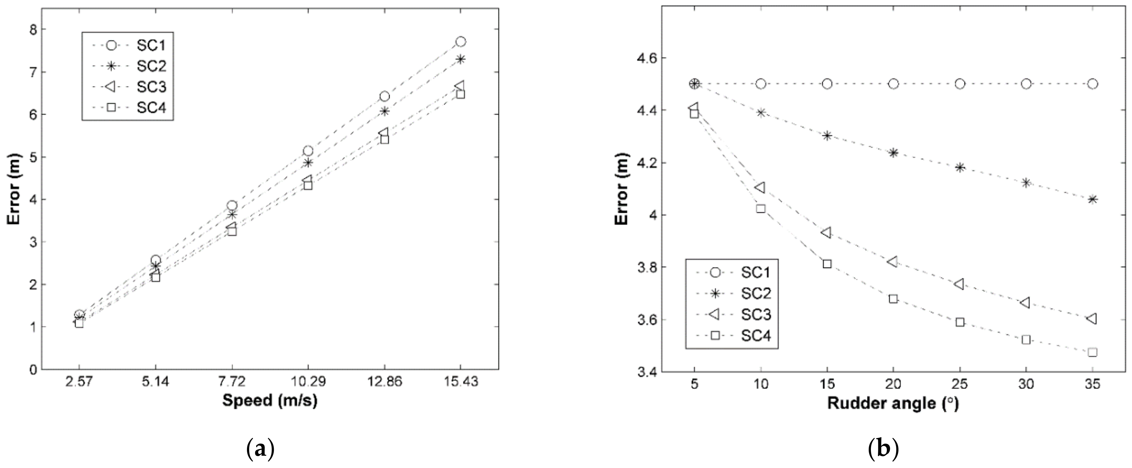
4.2.2. Error Analysis of Critical Latency Estimates

Figure 10 shows the estimation errors of critical latency for four scenarios. In Figure 10a, the errors with vessel speed changes are shown to increase as the vessel speed increases, while in Figure 10b, the errors with rudder angle changes decrease or become similar values as the rudder angle increases.

In four scenarios, the error appears to occur within 8 m. This value is small enough to correspond to one sample when a measurement error value of 7.72 m (0.5 × 15.43) is considered, which can result from the sampling time (0.5 s) applied to the OS trajectory measurement and the maximum vessel speed (15.43 m/s) given. As a result, the critical latency estimating method proposed in this study was verified to be partially effective.

4.3. Estimated Performance Evaluation of Critical Latency

The estimated performance of critical latency was evaluated by a visual analysis of the position and time between the collision point that can be caused by the designed route and the collision point that can be caused by turning. The estimated performance evaluation was carried out for each of the four scenarios.

4.3.1. Evaluation of Estimated Performance

The evaluation results of the estimated performance were described in the order from Scenario 4 with the largest encounter bearing to Scenario 1 with the smallest encounter bearing.

Figure 11 explains the estimated results for Scenario 4 (encountering angle of 135), given the initial conditions as follows; OS-TS initial relative distance of 2925 m, initial speed of both vessels ν1 (2.57 m/s).

Figure 11a shows the collision points estimated by the OS-TS encounter and critical latency. The solid-black, -blue, and -red lines represent the designed route of the OS (000° of heading), the designed route of the TS (315° of heading), and part of the turning circle, respectively. In addition, O, T, M, and C represent OS initial position, TS initial position, OS-TS collision position caused by turning maneuver of OS, and OS-TS collision position caused by designed route, respectively. ${\mathrm{S}}_{\mathrm{OS}}$ and ${\mathrm{S}}_{\mathrm{TS}}$ represent the turning start positions of the OS and TS, respectively.

Figure 11b shows the estimation result of the time of collision point C. If time t = 0 marks the start of the turn, then the relative distance at t = 0 for the DR and TC should be the same. The black and blue lines represent the OS-TS relative distance RD_DR by the designed path and the generated OS-TS relative distance ${\mathrm{RD}}_{\mathrm{TC}}$. ${\mathrm{RD}}_{\mathrm{TC}}$ seems to converge to 0 at point C (24.38 min).

Figure 12 relates to Scenario 3 (encountering angle of 90), given the initial conditions as follows.

OS-TS initial relative distance of 3095 m, initial speed of both vessels 1 (5 knots). The descriptions and the meaning of the symbols in Figure 12 are the same as in Figure 11. In Figure 12a, two collision points of OS-TS are shown. In Figure 12b, the OS-TS relative distance ${\mathrm{RD}}_{\mathrm{TC}}$ appears to converge at points M (11.21 min) and C (18.26 min), and the OS-TC relative distance ${\mathrm{RD}}_{\mathrm{DR}}$ appears earlier at point M than point C appears to be.

Figure 13 relates to Scenario 2 (encountering angle of 45), given the initial conditions as follows.

OS-TS initial relative distance of 33,265 m, initial speed of both vessels ν1 (5 knots). The descriptions and the meaning of the symbols in Figure 13 are the same as in Figure 11. In Figure 13a, two collision points of OS-TS are shown. In Figure 13b, OS-TS relative distance ${\mathrm{RD}}_{\mathrm{DR}}$ is shown to converge at 0 (zero) at Points M (10.82 min) and C (15.02 min), and it is shown to appear earlier at Point M than at Point C.

Figure 14 relates to Scenario 1 (1-degree head-on situation), given the initial conditions as follows.

OS-TS initial relative distance of 901 m, initial speed of both vessels ν1(5 knots). The descriptions of Figure 14a,b are the same as in Figure 11. In Figure 14a, two collision points of OS-TS are shown. As the encounter relative bearing in Scenario 1 is 1 degree, which is smaller than the previous three scenarios, the three points (S, M, and C) are shown to assemble near each other. In Figure 14b, OS-TS relative distance ${\mathrm{RD}}_{\mathrm{DR}}$ is shown to converge at 0 (zero) at Points M (7.08 min) and C (7.62 min), and it is shown to appear earlier at Point M than at Point C. In addition, the time difference between M and C was 0.54 min (7.62−7.08), which was the smallest in all scenarios.

4.3.2. Summary of Performance Evaluation Results

Performance evaluations for the four scenarios described in Section 4.3.1. demonstrated that the location of the two points of potential OS-TS collision—M and C—and the collision time can be estimated. A summary of the results is as follows:

• The time at both points decreases as the encounter bearing decreases;
• The time difference between the two points also decreases as the encounter bearing decreases;
• The smaller the time for two potential collision points and the smaller the time difference between the two points, the closer the collision is.

Therefore, the proposed technique is expected to be applicable for collision avoidance under COLREGs, which will be discussed thirdly in Section 5 (Discussion).

5. Discussion

The need for discussion was previously raised about the following:

• Consideration of vessel scale (length, width) in estimating critical latency;
• Consideration of turning circles that can be observed on actual vessels;
• Application of critical latency for collision avoidance in remote maneuvering.

The first point is about the vessel scale. The collision position of the OS-TS is theoretically the point at which the OS-TS relative distance is zero unless the vessel scale is considered; whereas, when the vessel scale is considered, the collision positions of the OS-TS are the points where the hulls of the two vessels can meet each other, which may appear complex depending on the encounter situation and vessel shape. This complexity can be an obstacle in applying vessel scale to critical latency estimation. The introduction of the ship domain concept, now widely applied in the maritime domain, can be considered as a solution. The concept defines the OS safety zone or the other ship safety zone where the two vessels can be safely separated to avoid collision [36,37,38,39]. The study of estimating critical latency introducing the concept of ship domain is put aside as a task to be studied later.

The second point is about the acquisition of turning circles. Turning circles are required by international regulations to be measured and posted on the bridge for a combination of certain speeds and rudder angles [10,35]. It is observed that turning circles for a combination of various vessel speeds and rudder angles must be obtained at real sea; however, this requires a lot of cost and time. A number of studies have been reported in the past on how to obtain turning circle data from numerical analysis using the current ship’s hydrodynamic model. [31,32,33]. In addition, it is reported that numerical simulation can be a method of evaluating remote maneuvers of autonomous vessels [3,4]. Therefore, the second point is considered as an issue to be addressed by comparing the turning circles measured using numerical simulations with some turning circles measured on actual vessels.

The third point is regarding the application of critical latency of collision avoidance. It was confirmed through the experiment that the critical latency estimation method proposed in this study is applicable to the estimation of the location and time at which two ships can collide. Using this result, it can be applied to the current ship domain and collision avoidance assessment. When the application of collision avoidance is considered in remote maneuvering, the method in this study needs to be concerned so that the OS-TS’s safety distance can be secured. According to Coldwell [39], it is known that the ship’s domain can be safely separated from the other ship’s length of 3.58 times the ship’s length. In addition, various studies that can secure the safety distance of OS-TS have been reported [23,24,27,28]. This will be left as a future task for this study.

An additional point to discuss is the extent to which the speed of the vessel affects the turning trajectory. The results rendered by the simulator mean that the ship’s circulation radius depends only on the angle of deflection of the rudder blade, and the otherwise obvious influence of the ship’s speed on the turning trajectory is not noticed. Further research in this area is considered necessary.

6. Conclusions

This study proposes a method of estimating critical latency that causes two vessels to collide to avoid collisions in remote maneuvering. The basic concept of critical latency was established by applying the turning circles formed by the ship’s turning, and based on this, critical latency was formulated using the radius of the turning circle and turning time ratio. Turning circle data were obtained through ship maneuvering simulations, and the estimated performance of critical latency was evaluated in the four designed scenarios. The study findings can be summarized as follows:

• In the case of the cargo vessel (171.8 m long, 23.17 m wide) applied to the experiment, the collision occurred with a critical latency having an average range of 0.2–8.53 min depending on the rudder angle and with a critical latency having an average range of 0.2–12.74 min depending on the vessel speed.
• Evaluation of the estimated performance of critical latency demonstrated that the collisions caused by the designed route and critical latency can be identified in terms of location and time.

As a result, the proposed method is expected to contribute to providing a clue to avoid ship collisions in remote maneuvering that may be caused by latency. In addition, the proposed method did not consider the scale of the vessel. In this regard, future studies about the method of considering the ship domain and collision avoidance assessment in estimating critical latency are required. It is expected to be conducted by introducing the ship domain concept [39] in which the two vessels can be safely separated in various encounter situations.

References

1. IMO. IMO Takes First Steps to Address Autonomous Ship. Available online: https://www.imo.org/en/MediaCentre/PressBriefings/Pages/08-MSC-99-MASS-scoping.aspx (accessed on 31 May 2018).
2. IMO. MSC.1/Circ.1638 of 3June 2021 “Outcome of the Regulatory Scoping Exercise for the use of Maritime Autonomous Surface; Ships (MASS): London, UK, 2021. [Google Scholar]
3. DNV-GL. Autonomous and Remotely Operated Ships; DNV-GL: Oslo, Norway, 2018; pp. 1–111. [Google Scholar]
4. ClassNK. Guidelines for Automated/Autonomous Operation on Ships (Ver. 1.0); ClassNK: Tokyo, Japan, 2020; pp. 1–40. [Google Scholar]
5. VTMIS. EU Operational Guidelines for Safe, Secure and Sustainable Trials of Maritime Autonomous Surface Ships (MASS); European Union: Maastricht, The Netherlands, 2020; pp. 1–23. [Google Scholar]
6. Rolls-Royce plc. Remote and Autonomous Ships the Next Steps; AAWA Position Paper; Rolls-Royce plc: London, UK, 2016; pp. 1–87. [Google Scholar]
7. Wariishi, K. Maritime Autonomous Surface Ships: Development Trends and Prospects–How Digitalization Drives Changes in Maritime Industry; Mitsui & Co. Global Strategic Studies Institute Monthly Report; Mitsui & Co. Global Strategic Studies Institute: Tokyo, Japan, 2019; pp. 1–8. [Google Scholar]
8. Chen, Y.Y.; Ellis-Tiew, M.; Chen, W.; Wang, C. Fuzzy risk evaluation and collision avoidance control of unmanned surface vessels. Appl. Sci. 2021, 11, 6338. [Google Scholar] [CrossRef]
9. Benjamin, M.R.; Leonard, J.J.; Curcio, J.A.; Newman, P.M. A method for protocol-based collision avoidance between autonomous marine surface craft. J. Field Robot. 2006, 23, 333–346. [Google Scholar] [CrossRef] [Green Version]
10. IMO. Convention on the International Regulations for Preventing Collisions at Sea; International Maritime Organization: London, UK, 1972. [Google Scholar]
11. Inoue, K. Theory and Practice of Ship Handling; Kobe University: Kobe, Japan, 2013; pp. 25–29. [Google Scholar]
12. Chauvin, C.; Lardjane, S.; Morel, G.; Clostermann, J.P.; Langard, B. Human and organisational factors in maritime accidents: Analysis of collisions at sea using the HFACS. Accid. Anal. Prev. 2013, 59, 26–37. [Google Scholar] [CrossRef] [PubMed]
13. Cordon, J.R.; Mestre, J.M.; Walliser, J. Human factors in seafaring: The role of situation awareness. Saf. Sci. 2017, 93, 256–265. [Google Scholar] [CrossRef]
14. Embrey, D. Understanding Human Behaviour and Error; Human Reliability Associates: Wigan, UK, 2005; pp. 1–10. [Google Scholar]
15. Yim, J.B.; Kim, D.S.; Park, D.J. Modeling perceived collision risk in vessel encounter situations. Ocean Eng. 2018, 166, 64–75. [Google Scholar] [CrossRef]
16. Szlapczynski, R. A unified measure of collision risk derived from the concept of a ship domain. J. Navig. 2006, 59, 477–490. [Google Scholar] [CrossRef]
17. Lee, H.J.; Furukawa, Y.; Park, D.J. Seafarers’ awareness-based domain modelling in restricted areas. J. Navig. 2021, 1–17. [Google Scholar] [CrossRef]
18. Szlapczynski, R.; Szlapczynska, J. A target information display for visualizing collision avoidance manoeuvres in various visibility conditions. J. Navig. 2015, 68, 1041–1055. [Google Scholar] [CrossRef]
19. Szlapczynski, R.; Szlapczynska, J. An analysis of domain-based ship collision risk parameters. Ocean Eng. 2016, 126, 47–56. [Google Scholar] [CrossRef]
20. Szlapczynski, R.; Szlapczynska, J. Review of ship safety domains: Models and applications. Ocean Eng. 2017, 145, 277–289. [Google Scholar] [CrossRef]
21. Szlapczynski, R.; Krata, P.; Szlapczynska, J. Ship domain applied to determining distances for collision avoidance manoeuvres in give-way situations. Ocean Eng. 2018, 165, 43–54. [Google Scholar] [CrossRef]
22. Fauville, G.; Queiroz, A.C.M.; Woolsey, E.S.; Kelly, J.W.; Bailenson, J.N. The effect of water immersion on vection in virtual reality. Sci. Rep. 2021, 11, 1022. [Google Scholar] [CrossRef] [PubMed]
23. Krata, P.; Montewka, J. Assessment of a critical area for a give-way ship in a collision encounter. Arch. Transp. 2015, 34, 51–60. [Google Scholar] [CrossRef] [Green Version]
24. Krata, P.; Montewka, J.; Hinz, T. Towards the assessment of critical area in a collision encounter accounting for stability conditions of a ship. Pr. Nauk. Politechn. Warsz. 2016, 114, 169–178. [Google Scholar]
25. Tanwar, S.; Tyagi, S.; Budhiraja, I.; Kumar, N. Tactile Internet for autonomous vehicles: Latency and reliability analysis. IEEE Wirel. Commun. 2019, 26, 66–72. [Google Scholar] [CrossRef]
26. Zhang, J.; Yan, X.; Chen, X.; Sang, L.; Zhang, D. A novel approach for assistance with anti-collision decision making based on the International Regulations for Preventing Collisions at Sea. Proc. Inst. Mech. Eng. Part M J. Eng. Marit. Environ. 2012, 226, 250–259. [Google Scholar] [CrossRef]
27. Szlapczynski, R. A new method of planning collision avoidance manoeuvres for multi-target encounter situations. J. Navig. 2018, 61, 307. [Google Scholar] [CrossRef]
28. Szlapczynski, R.; Szlapczynska, J. A ship domain-based model of collision risk for near-miss detection and Collision Alert Systems. Reliab. Eng. Syst. 2021, 214, 107766. [Google Scholar] [CrossRef]
29. Zhang, M.; Montewka, J.; Manderbacka, T.; Kujala, P.; Hirdaris, S. A big data analytics method for the evaluation of ship-ship collision risk reflecting hydrometeorological conditions. Reliab. Eng. Syst. 2021, 213, 107674. [Google Scholar] [CrossRef]
30. Wang, N. A novel analytical framework for dynamic quaternion ship domains. J. Navig. 2013, 66, 265–281. [Google Scholar] [CrossRef] [Green Version]
31. Chislett, M.S.; Strom-Tejsen, J. Planar motion mechanism tests and full-scale steering and manoeuvring predictions for a Mariner class vessel. Int. Shipbuild. Prog. 1965, 12, 201–224. [Google Scholar] [CrossRef]
32. Åström, K.J.; Källström, C.G. Identification of ship steering dynamics. Automatica 1976, 12, 9–22. [Google Scholar] [CrossRef] [Green Version]
33. Van Berlekom, W.B.; Goddard, T.A. Maneuvering of large tankers. Soc. Nav. Archit. Mar. Eng. 1972, 1, 25. [Google Scholar]
34. K-SIM Navigation. Available online: https://www.kongsberg.com/digital/products/maritime-simulation/k-sim-navigation/ (accessed on 16 June 2021).
35. Bowditch, N. Chapter 12-The sailings. In American Practical Navigator: An Epitome of Navigation; Clifford, G.J., Jr., Ed.; National Geospatial-Intelligence Agency: Springfield, VI, USA, 2019; pp. 193–213. [Google Scholar]
36. Davis, P.V.; Dove, M.J.; Stockel, C.T. A computer simulation of marine traffic using domains and arenas. J. Navig. 1980, 33, 215–222. [Google Scholar] [CrossRef]
37. Fujii, Y.; Tanaka, K. Traffic capacity. J. Navig. 1971, 24, 543–552. [Google Scholar] [CrossRef]
38. Goodwin, E.M. A statistical study of ship domains. J. Navig. 1975, 28, 328–344. [Google Scholar] [CrossRef] [Green Version]
39. Coldwell, T.G. Marine traffic behaviour in restricted waters. J. Navig. 1983, 36, 430–444. [Google Scholar] [CrossRef]
Figure 1. Description of relationship between own ship and target ship while introducing the turning circle of the own ship.
Applsci 11 10987 g001
Figure 2. Concept for estimating a critical latency.
Applsci 11 10987 g002
Figure 3. Four scenarios designed for evaluating the estimated performance of critical latency.
Applsci 11 10987 g003
Figure 4. Scene of ship maneuvering simulation for observing the turning circle.
Applsci 11 10987 g004
Figure 5. Flowchart summarizing the study procedures.
Applsci 11 10987 g005
Figure 6. Measurement of 42 trajectories of OS for combination of seven rudder angles and six vessel speeds.
Applsci 11 10987 g006
Figure 7. x- and y- positions of measured OS trajectories vs. turning time: (a) x-coordinate; (b) y-coordinate: vessel’s velocities: v1–v6 and rudder angles.
Applsci 11 10987 g007
Figure 8. OS trajectory data processing results for calculating turning time ratios: (a) turning circles with radius R; (b) trajectory shifted to the coordinate center (0,0); (c) x-axis scale differences between turning circles and trajectories; (d) y-axis scale differences between turning circles and trajectories; (e) turning angle differences between turning circles and trajectories; (f) turning time ratio ROT.
Applsci 11 10987 g008
Figure 9. Average value of estimated critical latency for four scenarios: (a) Scenario 1; (b) Scenario 2; (c) Scenario 3; (d) Scenario 4.
Applsci 11 10987 g009
Figure 10. Estimation error of critical latency for each of six vessel speeds and seven rudder angles: (a) error for six vessel speeds in four scenarios; (b) error for seven rudder angles in four scenarios.
Applsci 11 10987 g010
Figure 11. Estimation results for Scenario 4 (encountering angle of 135): (a) OS-TS encounter and collision points; (b) Estimation of the OS-TS relative distance and the time at collision Points C and M over time.
Applsci 11 10987 g011
Figure 12. Estimation results for Scenario 3 (encountering angle of 90): (a) OS-TS encounter and collision points; (b) Estimation of the OS-TS relative distance and the time at collision Points C and M over time.
Applsci 11 10987 g012
Figure 13. Estimation results for Scenario 2 (encountering angle of 45): (a) OS-TS encounter and collision points; (b) Estimation of the OS-TS relative distance and the time at collision Points C and M over time.
Applsci 11 10987 g013
Figure 14. Estimation results for Scenario 1 (1-degree head-on situation): (a) OS-TS encounter and collision points; (b) Estimation of the OS-TS relative distance and the time at collision Points C and M over time.
Applsci 11 10987 g014