
Traffic Signal Optimization for Multiple Intersections Based on Reinforcement Learning


Abstract
:1. Introduction
2. Literature Review
3. Methods
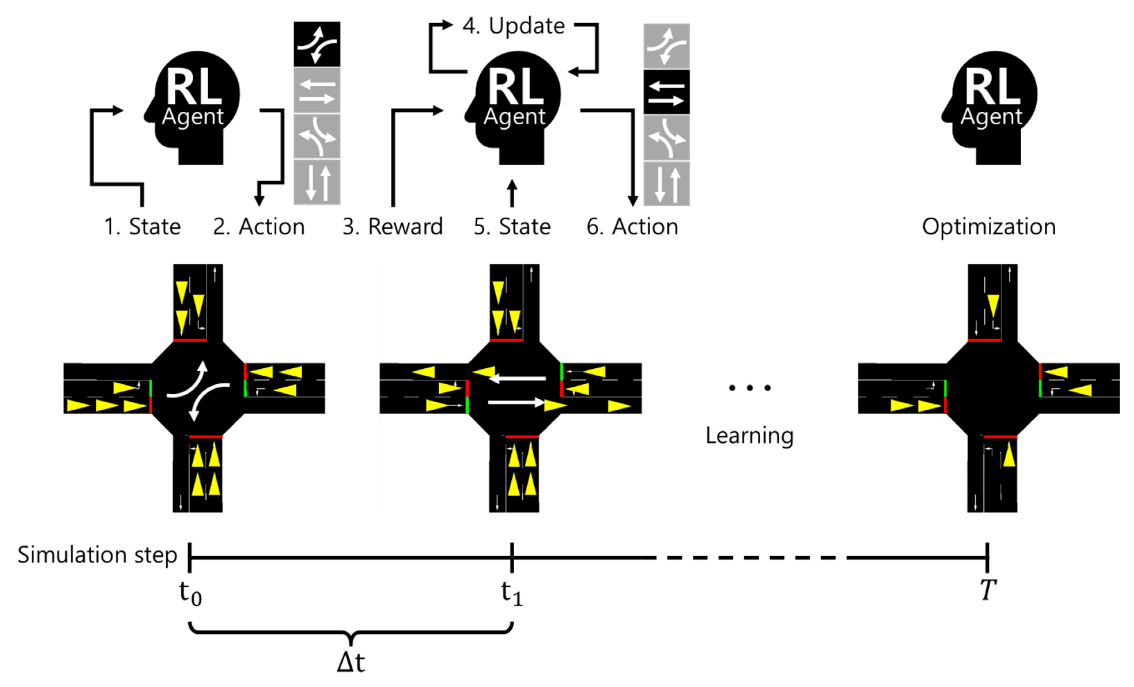
3.1. Learning Process
3.2. State
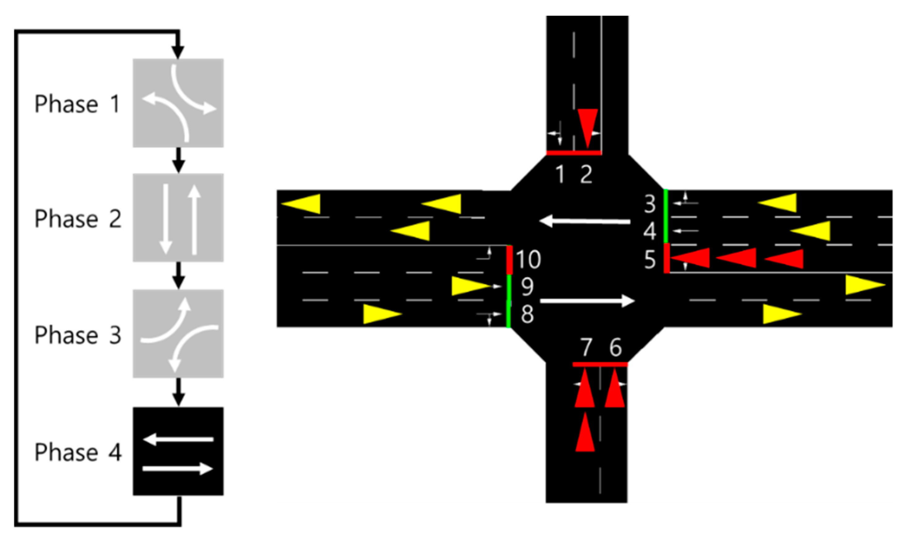
3.3. Action
3.4. Reward
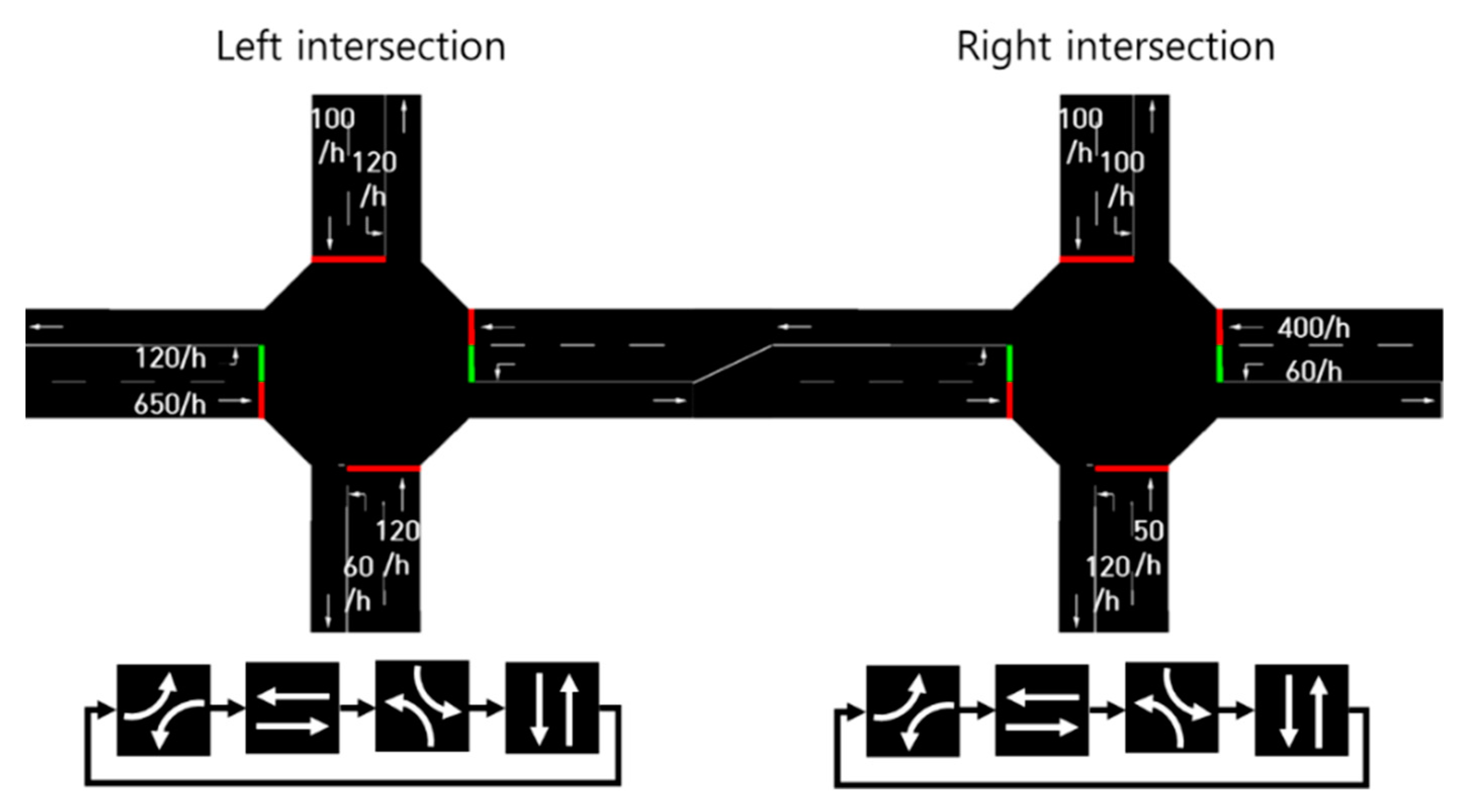
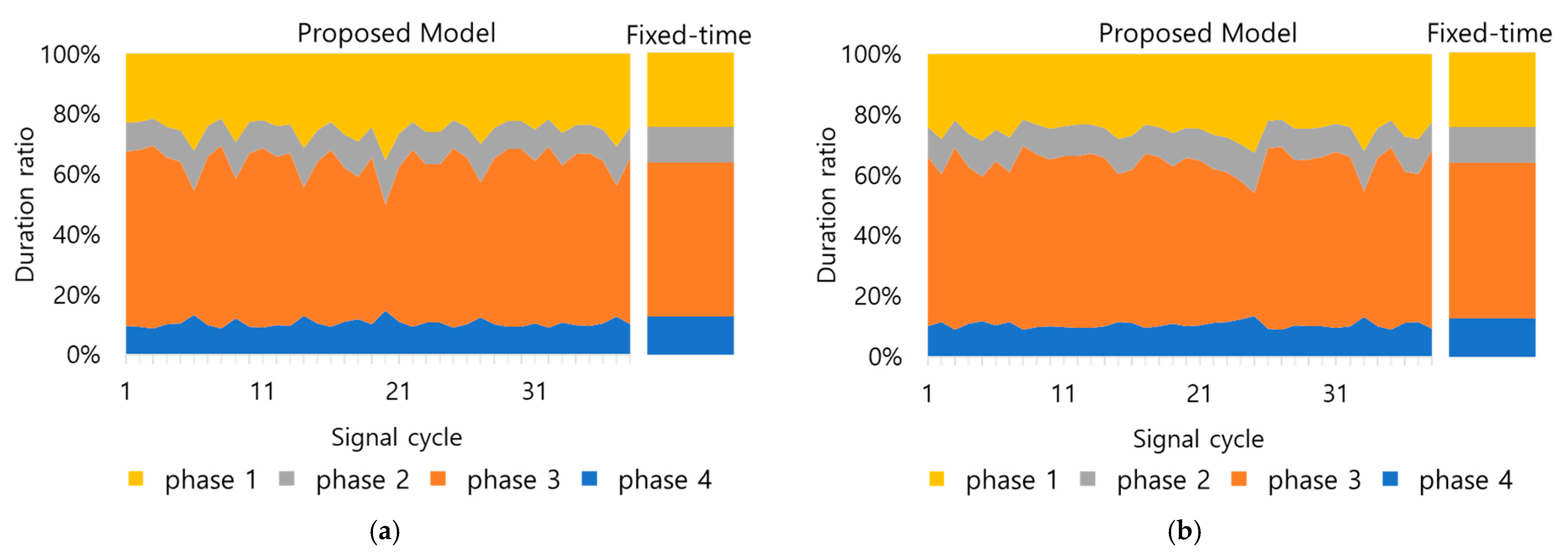
4. Simulation
4.1. Scenario 1
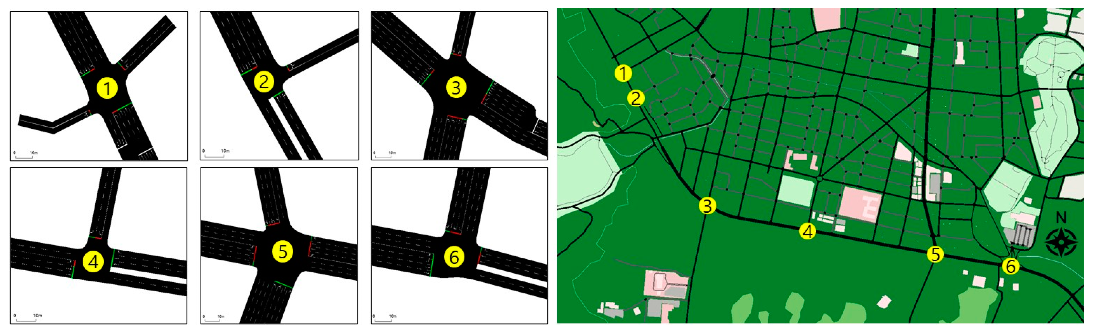
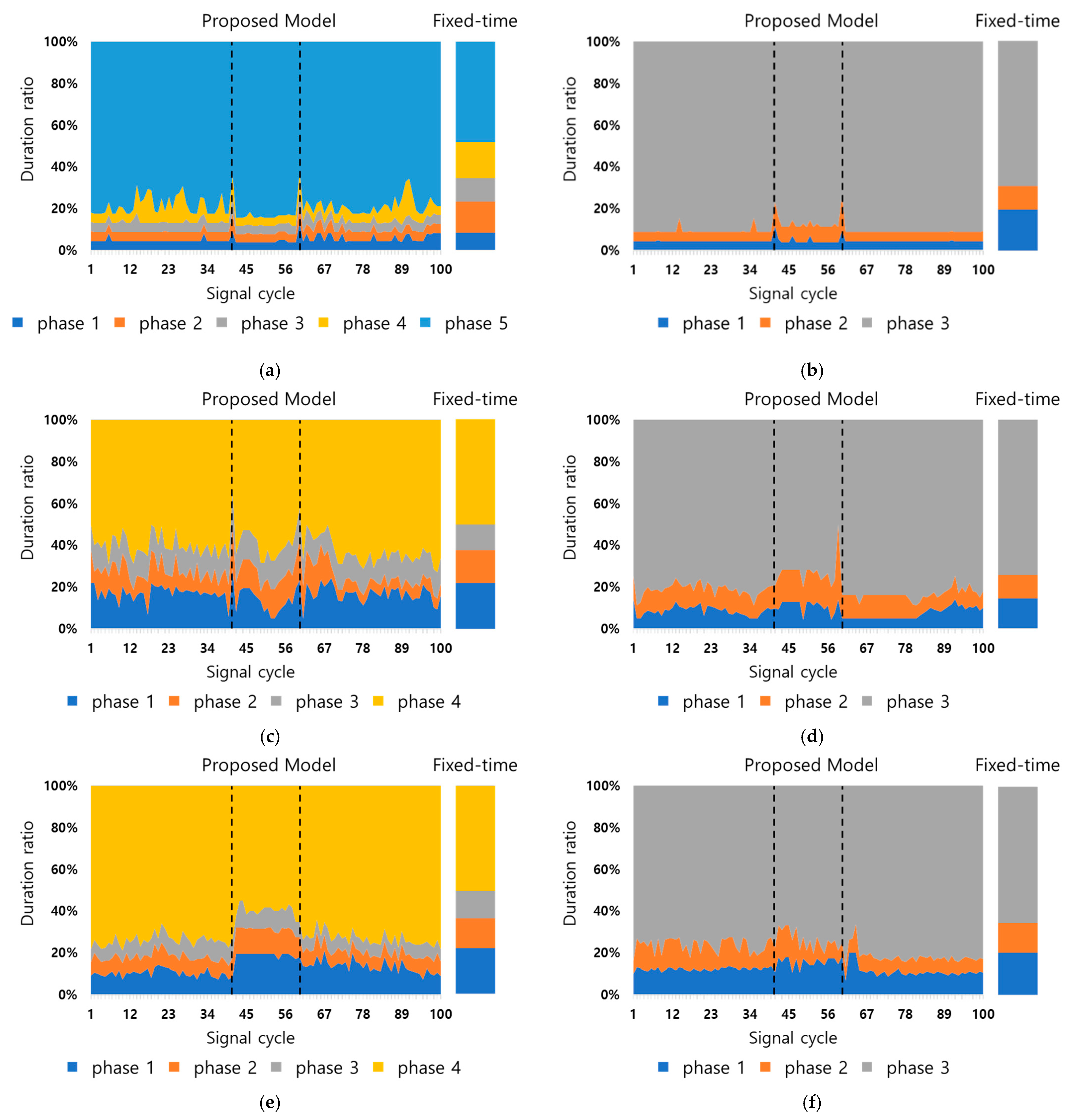
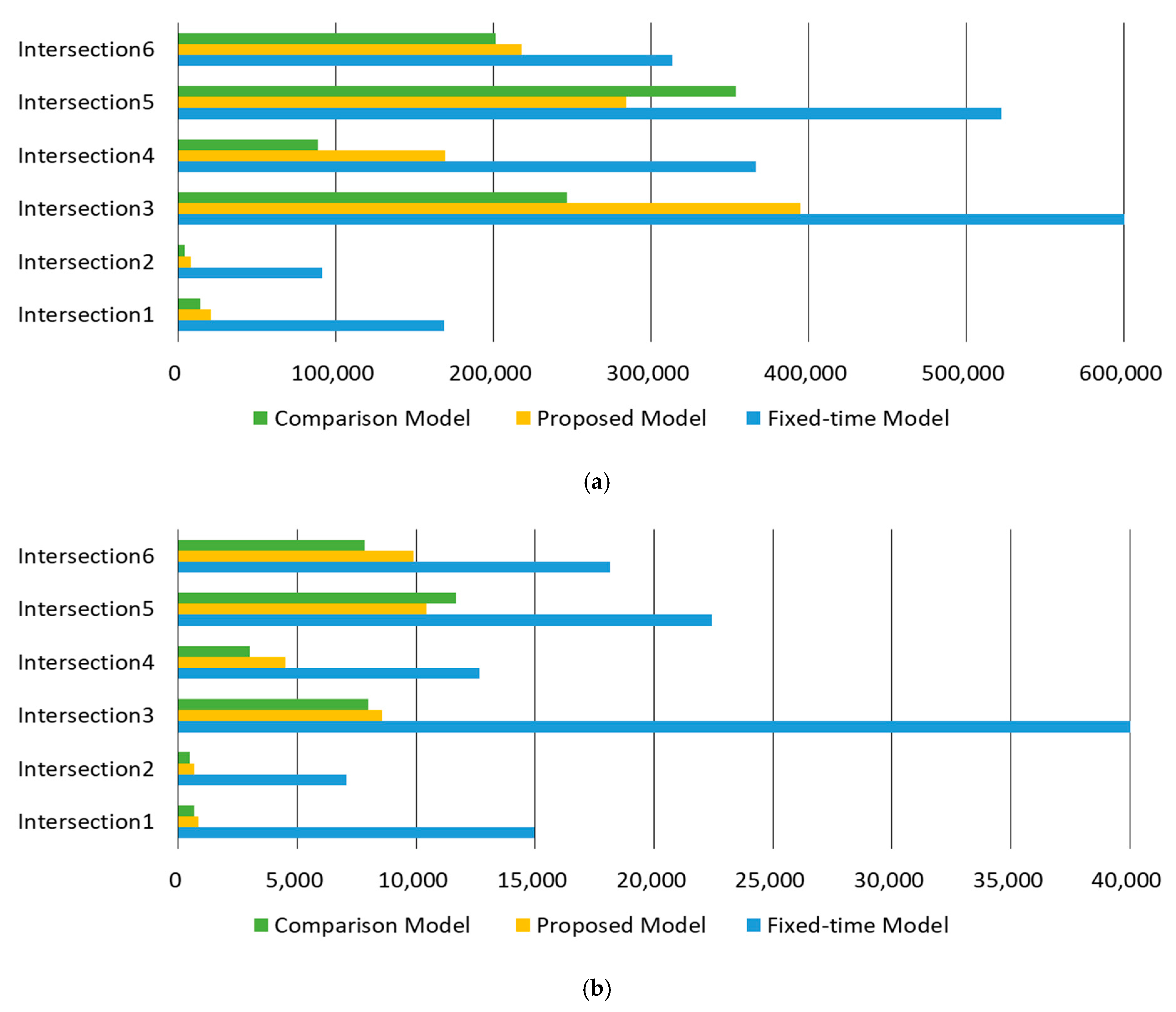
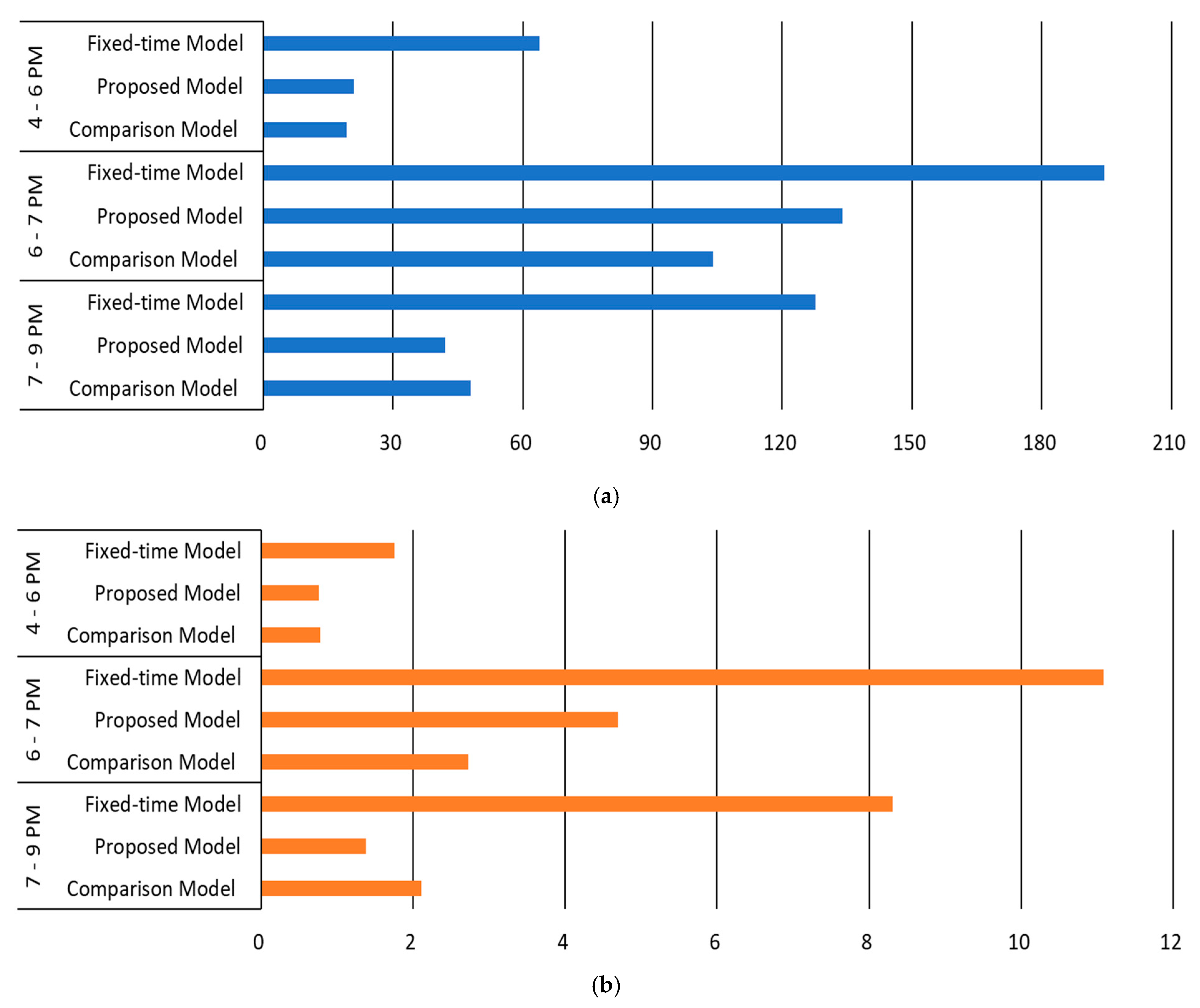
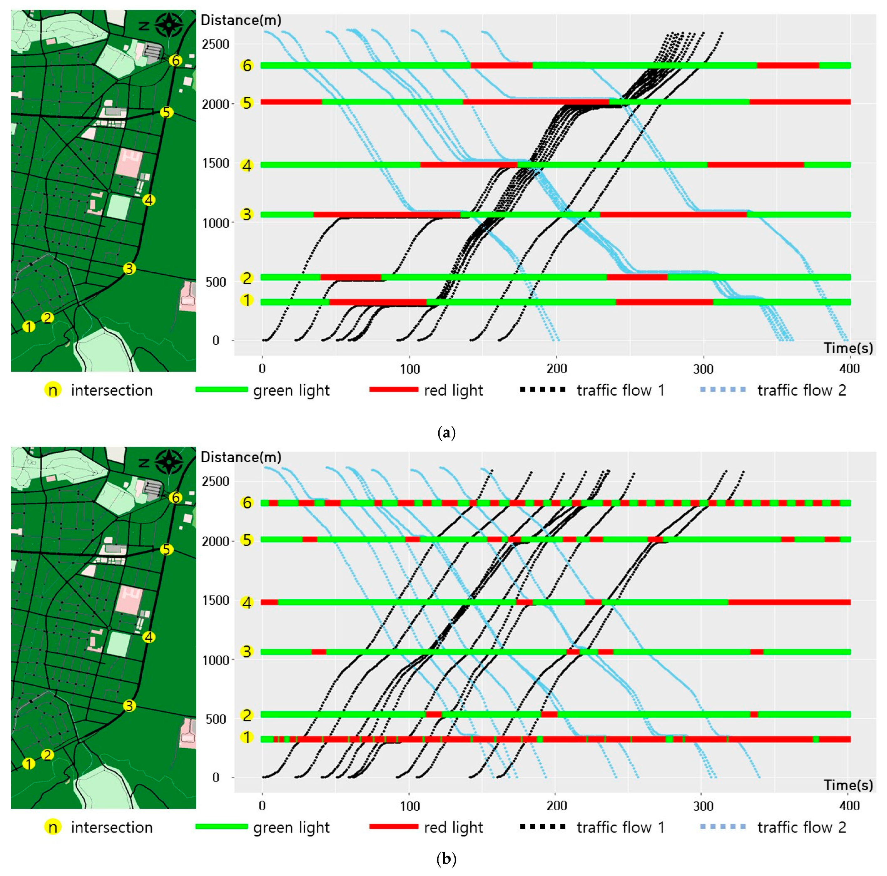
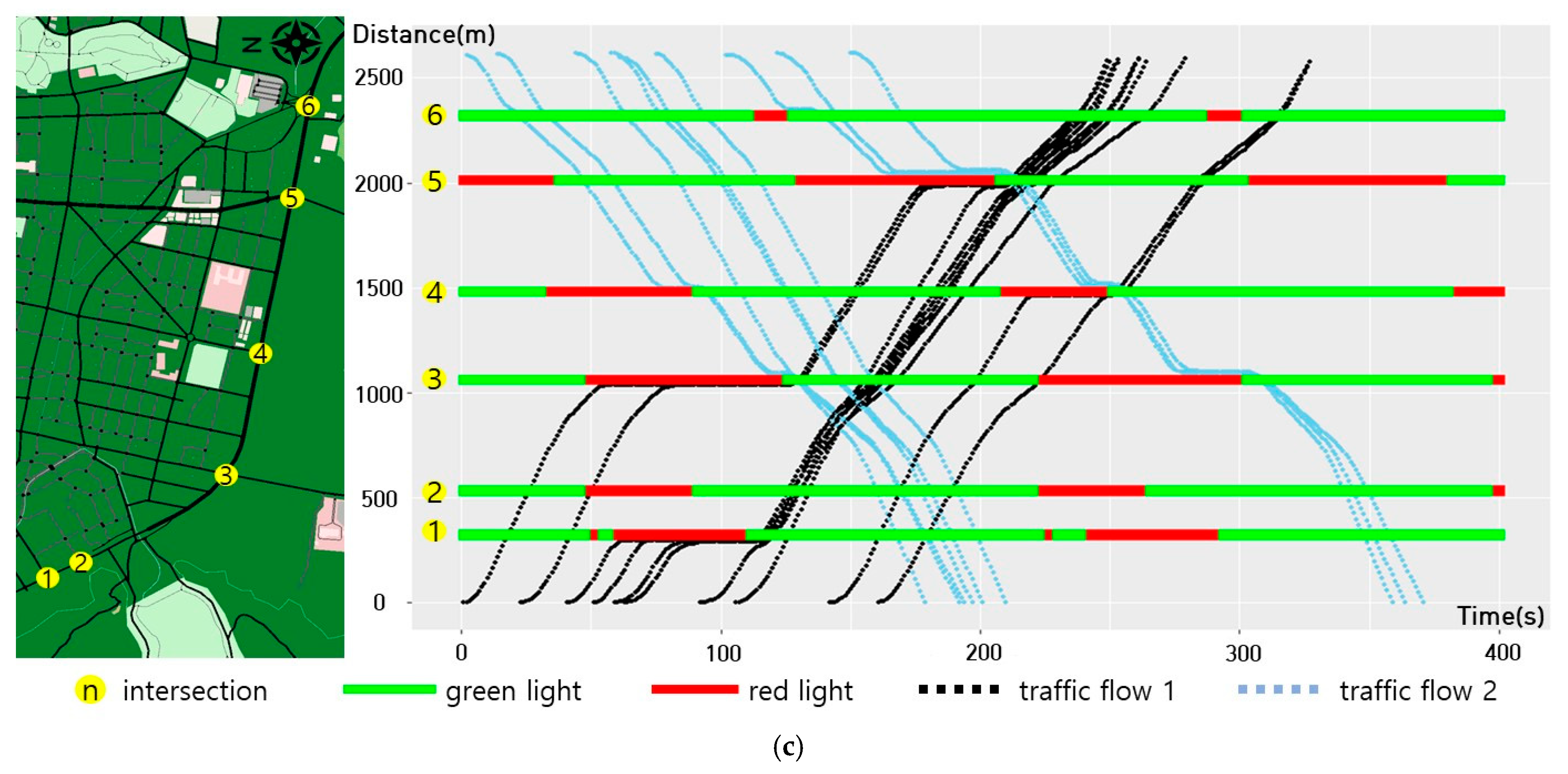
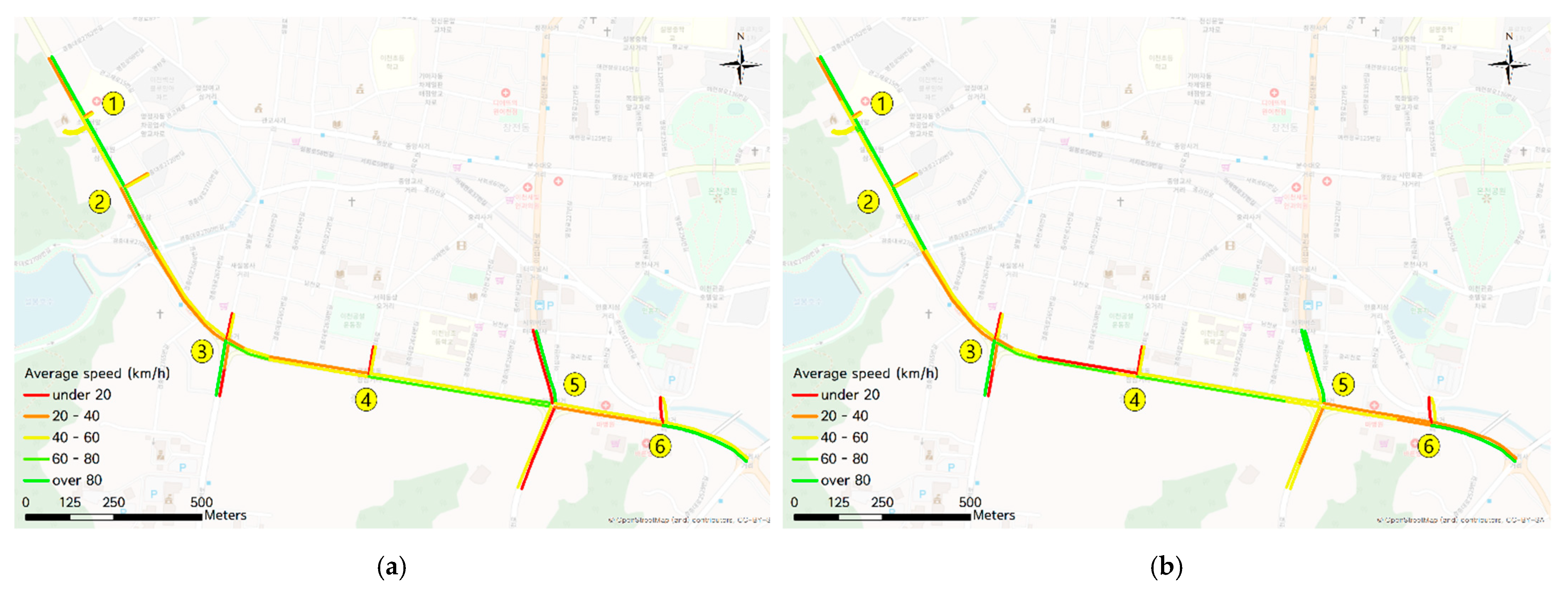
4.2. Scenario 2
5. Conclusions
Author Contributions
Funding
Institutional Review Board Statement
Informed Consent Statement
Data Availability Statement
Conflicts of Interest
References
- Han, Y.; Kim, Y. Spatiotemporal congestion recognition index to evaluate performance under oversaturated conditions. KSCE J. Civil Eng. 2019, 23, 3714–3723. [Google Scholar] [CrossRef]
- Yang, S.; Yang, B.; Wong, H.-S.; Kang, Z. Cooperative traffic signal control using multi-step return and off-policy asynchronous advantage actor-critic graph algorithm. Knowl. Based Syst. 2019, 183, 104855. [Google Scholar] [CrossRef]
- Aslani, M.; Mesgari, M.S.; Seipel, S.; Wiering, M. Developing adaptive traffic signal control by actor–critic and direct exploration methods. Proc. Inst. Civ. Eng. Transp. 2019, 172, 289–298. [Google Scholar] [CrossRef]
- Aslani, M.; Stefan, S.; Marco, W. Continuous residual reinforcement learning for traffic signal control optimization. Can. J. Civ. Eng. 2018, 45, 690–702. [Google Scholar] [CrossRef]
- Mannion, P.; Duggan, J.; Howley, E. An experimental review of reinforcement learning algorithms for adaptive traffic signal control. Auton. Road Transp. Support Syst. 2016, 4, 47–66. [Google Scholar] [CrossRef]
- Li, L.; Lv, Y.; Wang, F.-Y. Traffic signal timing via deep reinforcement learning. IEEE/CAA J. Autom. Sin. 2016, 3, 247–254. [Google Scholar]
- Ge, H.; Song, Y.; Wu, C.; Ren, J.; Tan, G. Cooperative deep q-learning with q-value transfer for multi-intersection signal control. IEEE Access 2019, 7, 40797–40809. [Google Scholar] [CrossRef]
- Al Islam, S.B.; Hajbabaie, A. Distributed coordinated signal timing optimization in connected transportation networks. Transp. Res. Part C Emerg. Technol. 2017, 100, 272–285. [Google Scholar] [CrossRef]
- Mousavi, S.S.; Schukat, M.; Howley, E. Traffic light control using deep policy-gradient and value-function-based reinforcement learning. IET Intell. Transp. Syst. 2017, 11, 417–423. [Google Scholar] [CrossRef] [Green Version]
- Rasheed, F.; Yau, K.L.A.; Low, Y.C. Deep reinforcement learning for traffic signal control under disturbances: A case study on Sunway city, Malaysia. Future Gener. Comput. Syst. 2020, 109, 431–445. [Google Scholar] [CrossRef]
- Sutton, R.S.; Barto, A.G. Reinforcement Learning: An Introduction; MIT Press: Cambridge, MA, USA, 2018. [Google Scholar]
- Touhbi, S.; Babram, M.A.; Nguyen-Huu, T.; Marilleau, N.; Hbid, M.L.; Cambier, C.; Stinckwich, S. Adaptive traffic signal control: Exploring reward definition for reinforcement learning. Procedia Comput. Sci. 2017, 109, 513–520. [Google Scholar] [CrossRef]
- Liang, X.; Du, X.; Wang, G.; Han, Z. Deep reinforcement learning for traffic light control in vehicular networks. Mach. Learn. 2018, 68, 1–11. [Google Scholar] [CrossRef] [Green Version]
- Wang, S.; Xie, X.; Huang, K.; Zeng, J.; Cai, Z. Deep reinforcement learning-based traffic signal control using high-resolution event-based data. Entropy 2019, 21, 744. [Google Scholar] [CrossRef] [Green Version]
- Gong, Y.; Abdel-Aty, M.; Cai, Q.; Rahman, M.S. Decentralized network level adaptive signal control by multi-agent deep reinforcement learning. Transp. Res. Interdiscip. Perspect. 2019, 9, 10306–10316. [Google Scholar] [CrossRef]
- Chu, T.; Wang, J.; Codecà, L.; Li, Z. Multi-agent deep reinforcement learning for large-scale traffic signal control. IEEE Trans. Intell. Transp. Syst. 2019, 21, 1086–1095. [Google Scholar] [CrossRef] [Green Version]
- Egea, A.C.; Howell, S.; Knutins, M.; Connaughton, C. Assessment of Reward Functions for Reinforcement Learning Traffic Signal Control under Real-World Limitations. In Proceedings of the 2020 IEEE International Conference on Systems, Man, and Cybernetics (SMC), Totonto, ON, Canada, 11–14 October 2020; pp. 965–972. [Google Scholar]
- Ozan, C.; Baskan, O.; Haldenbilen, S.; Ceylan, H. A modified reinforcement learning algorithm for solving coordinated signalized networks. Transp. Res. Part C Emerg. Technol. 2015, 54, 40–55. [Google Scholar] [CrossRef]
- Kim, D.; Jeong, O. Cooperative traffic signal control with traffic flow prediction in multi-intersection. Sensors 2020, 20, 137. [Google Scholar] [CrossRef] [PubMed] [Green Version]
- Yuan, J.; Abdel-Aty, M.; Gong, Y.; Cai, Q. Real-time crash risk prediction using long short-term memory recurrent neural network. Transp. Res. Rec. 2019, 2673, 314–326. [Google Scholar] [CrossRef]
- Zhao, Y.; Liang, Y.; Hu, J.; Zhang, Z. Traffic Signal Control for Isolated Intersection Based on Coordination Game and Pareto Efficiency. In Proceedings of the 2019 IEEE Intelligent Transportation Systems Conference, Auckland, New Zealand, 27–30 October 2019; pp. 3508–3513. [Google Scholar] [CrossRef]
- Kühnel, N.; Theresa, T.; Kai, N. Implementing an adaptive traffic signal control algorithm in an agent-based transport simulation. Procedia Comput. Sci. 2018, 130, 894–899. [Google Scholar] [CrossRef]


| Parameters | Scenario 1 | Scenario 2 |
|---|---|---|
| Number of episodes | 100 | 160 |
| Simulation time of one episode (second) | 3600 | 18,000 |
| Time interval (second) | 3 | 3 |
| Learning rate | 0.0001 | 0.0001 |
| Number of intersections | 2 | 6 |
Publisher’s Note: MDPI stays neutral with regard to jurisdictional claims in published maps and institutional affiliations. |
© 2021 by the authors. Licensee MDPI, Basel, Switzerland. This article is an open access article distributed under the terms and conditions of the Creative Commons Attribution (CC BY) license (https://creativecommons.org/licenses/by/4.0/).
Share and Cite
Gu, J.; Lee, M.; Jun, C.; Han, Y.; Kim, Y.; Kim, J. Traffic Signal Optimization for Multiple Intersections Based on Reinforcement Learning. Appl. Sci. 2021, 11, 10688. https://doi.org/10.3390/app112210688
Gu J, Lee M, Jun C, Han Y, Kim Y, Kim J. Traffic Signal Optimization for Multiple Intersections Based on Reinforcement Learning. Applied Sciences. 2021; 11(22):10688. https://doi.org/10.3390/app112210688
Chicago/Turabian StyleGu, Jaun, Minhyuck Lee, Chulmin Jun, Yohee Han, Youngchan Kim, and Junwon Kim. 2021. "Traffic Signal Optimization for Multiple Intersections Based on Reinforcement Learning" Applied Sciences 11, no. 22: 10688. https://doi.org/10.3390/app112210688