
Self-Tuning Lam Annealing: Learning Hyperparameters While Problem Solving


Computer Science, Stockton University, 101 Vera King Farris Dr, Galloway, NJ 08205, USA
Appl. Sci. 2021, 11(21), 9828; https://doi.org/10.3390/app11219828
Submission received: 15 September 2021
/
Revised: 13 October 2021
/
Accepted: 19 October 2021
/
Published: 21 October 2021
(This article belongs to the Topic Machine and Deep Learning)
Abstract
:The runtime behavior of Simulated Annealing (SA), similar to other metaheuristics, is controlled by hyperparameters. For SA, hyperparameters affect how “temperature” varies over time, and “temperature” in turn affects SA’s decisions on whether or not to transition to neighboring states. It is typically necessary to tune the hyperparameters ahead of time. However, there are adaptive annealing schedules that use search feedback to evolve the “temperature” during the search. A classic and generally effective adaptive annealing schedule is the Modified Lam. Although effective, the Modified Lam can be sensitive to the scale of the cost function, and is sometimes slow to converge to its target behavior. In this paper, we present a novel variation of the Modified Lam that we call Self-Tuning Lam, which uses early search feedback to auto-adjust its self-adaptive behavior. Using a variety of discrete and continuous optimization problems, we demonstrate the ability of the Self-Tuning Lam to nearly instantaneously converge to its target behavior independent of the scale of the cost function, as well as its run length. Our implementation is integrated into Chips-n-Salsa, an open-source Java library for parallel and self-adaptive local search.
Keywords:
Self-Tuning; Simulated Annealing; Modified Lam; hyperparameters; Exponential Moving Average; adaptive search; metaheuristics; self-adaptive; optimization; open-sourcePACS:
02.70.-c; 07.05.Mh; 89.20.FfMSC:
68T05; 68T20; 68W50; 90C27; 90C591. Introduction
Optimization problems of industrial relevance are often NP-Hard, such as applications of various classical problems such as the optimization variants of NP-Complete problems like the traveling salesperson, graph coloring, largest common subgraph, and bin packing, among many others [1].
Approaches that are guaranteed to provide optimal solutions to such problems have worst case run-times that are exponential. Thus, it is common to turn to metaheuristics, such as genetic algorithms [2] and other forms of evolutionary computation, simulated annealing [3,4,5], tabu search [6], ant colony optimization [7], stochastic local search [8], among many others. Metaheuristics offer a trade-off between time and solution quality. Although not guaranteed to optimally solve the problem, they can often find near optimal solutions, or at least sufficiently optimal solutions, in a fraction of the time of the alternatives. They are also usually characterized by an anytime [9] property, where solution quality improves with additional runtime. Thus, one can run such an algorithm as long as time allows, utilizing whatever solution is found at the time it is needed.
In this paper, we specifically concern ourselves with Simulated Annealing (SA). Kirkpatrick, Gelatt, and Vecchi introduced SA several decades ago [3]. Since then, it has been applied to optimization problems from a variety of industries, such as in transportation [10,11], assembly lines [12], machine vision [13], path planning for robotics [14,15], networking [16,17], wireless sensor networks [18,19], scheduling [20], manufacturing [21], software testing [22,23], and industrial cutting [24], among many others. SA is a stochastic local search algorithm inspired by an analogy to the metallurgic process of annealing, where a metal is heated and then slowly cooled until it achieves a state of equilibrium. As a local search algorithm, SA iteratively generates random neighbors of the current solution configuration. A random neighbor with a cost that is equal to or better than that of the current solution is accepted. A random neighbor with a cost that is worse than that of the current solution may still be accepted, but the decision is randomized and depends upon the cost difference and a temperature parameter. The higher the temperature, the higher the probability that a random neighbor will be accepted. Near the end of a run of SA, when temperature is low, the probability of accepting a neighbor of higher cost than the current solution becomes low. Algorithm 1 provides pseudocode for the basic form of SA.
| Algorithm 1 Simulated Annealing |
|
SA uses the Boltzmann distribution in deciding whether to accept a randomly chosen neighbor . Specifically, if the cost of the random neighbor is less than or equal to the cost of the current solution S, then it definitely accepts the neighbor. SA always accepts neighbors that are not worse than the current solution. Otherwise, if the cost of the neighbor is higher than the cost of the current solution, the neighbor is accepted with probability, (line 10 of Algorithm 1).
The temperature T of the SA changes during the run (line 12 of Algorithm 1). The component of SA that controls the change of temperature is known as the annealing schedule, and there are several common annealing schedules such as exponential cooling (, where is a cooling rate less than, but usually near, 1.0, such as 0.95), linear cooling (, where is a parameter), and logarithmic cooling (, where i is the iteration number, and c and d are parameters). All of these start the temperature at some initially “high” value (line 7 of Algorithm 1) and then monotonically decrease it during the run. However, what qualifies as “high”, and how quickly the temperature should decrease (values for the hyperparameters, , , c, d of the various annealing schedules), may vary from one problem to another, and perhaps even from one instance to another. Good choices for these also likely depends upon the amount of time you have available to solve your problem. If you have much time available, then you might start with a higher temperature, and use a slower rate of cooling, than you would if you had very little time available. If you utilize one of these classic annealing schedules, then you will need to tune the hyperparameters ahead of time in some way using problem instances representative of the instances that you expect to encounter for your application. However, if the assumptions that you make about expected future instances vary much from what you actually later encounter in practice, then your SA may perform significantly below its capability.
As an alternative to one of the classic annealing schedules, several researchers have developed adaptive annealing schedules [25,26,27,28,29,30,31,32], imparting upon SA the ability to self-adjust the temperature during the run utilizing problem solving feedback to learn to improve performance. A recent example is Hubin’s hybrid of an adaptive SA with expectation-maximization for inference in hidden Markov models [26]. Another example is the approach by Bezáková et al, which accelerates the rate of cooling as the temperature decreases [29]. Cicirello observed that many adaptive annealing schedules assume that you at least know how much time is available for the run, but if that assumption is incorrect then SA may either spend too much time in a random walk (e.g., if much less time is available than you thought), or converge too quickly to local optima (e.g., if much more time is available than you thought). This observation leads Cicirello to introduce an approach that adapts the run length of SA over the course of a sequence of restarts, both in the sequential case as well as for a parallel SA [27]. Lam and Delosme’s early work on adaptive simulated annealing dynamically adjusts the size of the neighborhood function to attempt to follow a theoretically determined trajectory of the rate of neighbor acceptance, while using a monotonically decreasing temperature [32]. This has become known as Lam annealing. Swartz later modified Lam and Delosme’s approach to keep the neighborhood function fixed, and instead allows the temperature to fluctuate up and down throughout the run as necessary in order to keep the SA run on the acceptance rate trajectory of Lam and Delosme’s approach [31]. Boyan refined Swartz’s approach into what is now known as the Modified Lam [30], and which was then later further optimized by Cicirello [25]. We provide complete algorithmic details of the Modified Lam in Section 2.1 since it forms the foundation of our approach.
Our primary contribution is a new adaptive annealing schedule that we call the Self-Tuning Lam. The Self-Tuning Lam builds upon the Modified Lam, and is designed to overcome its limitations. The Modified Lam is often described as parameter-free [33]. However, it has several constants, whose values are argued to suffice across most problems. However, in reality, these constants should really be treated as algorithm hyperparameters [34], whose values can affect either quality of final solution or convergence speed or both. For example, the Modified Lam is sensitive to the scale of cost differences between neighboring solutions in the search space. If the run length is sufficiently long, the Modified Lam will eventually adapt its behavior to the scale of the cost function, but it can be slow in doing so. Our new Self-Tuning Lam annealing schedule uses feedback from the early portion of the search to self-learn the algorithm hyperparameters, adjusting to the scale of cost differences between neighboring solutions. Using a variety of discrete and continuous optimization problems, we show that the effects of our approach is an adaptive annealing schedule that nearly instantaneously converges to the target behavior (i.e., Lam and Delosme’s idealized acceptance rate trajectory) and maintains that target behavior throughout the run.
Additionally, we have contributed our Java implementation of the Self-Tuning Lam to Chips-n-Salsa. Chips-n-Salsa is an existing open-source library of stochastic local search algorithms whose key features include self-adaptive as well as parallel search [35]. The source code for Chips-n-Salsa is hosted on GitHub https://github.com/cicirello/Chips-n-Salsa (accessed on 16 September 2021); and regular releases are deployed to the Maven Central repository https://search.maven.org/artifact/org.cicirello/chips-n-salsa (accessed on 16 September 2021), from which practitioners can easily import the library using popular build tools. More details about the library, including API documentation, are available via the Chips-n-Salsa website https://chips-n-salsa.cicirello.org/ (accessed on 16 September 2021). By integrating our new annealing schedule into an existing library, we increase the potential impact of our research, enabling others to easily build upon our work.
To enable reproducibility [36], we released all of the source code of our experiments, the raw data of our experiments, as well as the source code implemented to analyze the data and to generate all of the figures of this paper. This is all available on GitHub https://github.com/cicirello/self-tuning-lam-experiments (accessed on 13 October 2021).
The remainder of this paper is organized as follows. We present our approach in Section 2, in which we begin by detailing the original Modified Lam annealing schedule, and then providing the algorithmic details of our new Self-Tuning Lam. Then, in Section 3, we empirically compare the behavior of the Self-Tuning Lam to the original Modified Lam on a variety of benchmarking problems, including both discrete optimization and continuous function optimization, as well as an NP-Hard problem. The aim of our experiments is not to demonstrate that our approach is superior to the original Modified Lam. After all, the No Free Lunch Theorem [37] indicates that any two optimization algorithms are equivalent if performance is measured over all possible problems. Rather, the aim of our experiments is to demonstrate that the Self-Tuning Lam, independent of run length and independent of cost function scale, consistently achieves and maintains the target behavior of Lam and Delosme’s idealized acceptance rate trajectory. Whether that target behavior more effectively solves the problem varies; and in our discussion of the results, we explain the problem characteristics that impacts problem solving performance. We wrap up with further discussion and conclusions in Section 4.
2. Methods
We begin this section with a detailed description of the original Modified Lam (Section 2.1). We then extract several hyperparameters (Section 2.2), whose values are treated by the Modified Lam as predefined constants rather than algorithm hyperparameters to tune. Then we present the details of our new Self-Tuning Lam (Section 2.3) showing how we can auto-adjust these hyperparameters during the run of SA.
2.1. Modified Lam
At the heart of our approach is an existing adaptive annealing schedule known as the Modified Lam. The Modified Lam is based on the empirical work of Lam and Delosme [32], where they studied the behavior of SA over a variety of optimization problems, and observed that during optimal runs the rate at which SA chooses to keep neighboring solutions tends to follow a common trajectory. Specifically, at the beginning of an optimal run, SA accepts nearly all neighbors, but the acceptance rate declines rapidly during the first 15% of the run when it settles upon an acceptance rate of 44%, which it maintains for the next 50% of the run. During the last 35% of the run, the acceptance rate rapidly declines as it converges to a solution. They found that this acceptance rate trajectory effectively balances the trade-off between exploring the search-space and exploiting observed regions of better-quality solutions. The optimal runs under observation are prohibitively long to be of practical use. However, Lam and Delosme went a step further and used their observations to derive an adaptive SA that attempts to replicate the acceptance rate behavior of an optimal run, but for a run of predetermined length. Lam and Delosme’s approach decreases the temperature monotonically, similar to classic annealing schedules, but uses a variable-sized neighborhood. During the run, if the current acceptance rate is below the target rate, they increase the size of the neighborhood; while if it is above the target rate, they decrease the size of the neighborhood.
One of the main drawbacks of Lam and Delosme’s [32] approach is the practicality of defining the neighborhood of a solution in a way that enables easily changing its size. This lead Swartz to an alternative approach to matching the idealized target rate of acceptance. Swartz suggested keeping the neighborhood function fixed, and allowing the temperature to fluctuate both up and down (rather than strictly decreasing) in order to attempt to match the target acceptance rate [31]. Boyan later provided a practical instantiation of what is now the Modified Lam [30]. Boyan’s Modified Lam requires the run length (in number of SA iterations) as an input. The Modified Lam then defines the target acceptance rate for iteration i, and for an SA run N iterations in length, as follows:
This leads to exponentially declining acceptance rates for the first 15% and the final 35% of the run, and a constant acceptance rate of 0.44 for the other 50% of the run. This Lam target acceptance rate is shown in Figure 1.
Boyan’s Modified Lam estimates the actual acceptance rate throughout the run using an Exponential Moving Average as follows (i again is the iteration number):
and where .
The initial temperature , and the temperature is updated during iteration i depending upon whether the estimated acceptance rate is higher or lower than the target rate as follows:
Recently, Cicirello made some further enhancements, including incremental calculation of the for iteration i from that of iteration , into what he called the Optimized Modified Lam [25], which is shown in pseudocode form in Algorithm 2. Cicirello’s Optimized Modified Lam follows the same target acceptance rate sequence as Boyan’s version, but requires only two exponentiations for the entire run, while the original version requires exponentiations, for a substantial time savings, especially for long runs. For multistart SA, the savings are even more significant, in that the Optimized Modified Lam requires only two exponentiations total during R restarts (provided run length for all R restarts is the same), whereas the original requires exponentiations. The Optimized Modified Lam is the current default annealing schedule in the open source Chips-n-Salsa library [35]. From this point onward, whenever we indicate Modified Lam, we specifically refer to this optimized version; and this is the version with which we compare the new Self-Tuning Lam later in the experiments of Section 3.
| Algorithm 2 Optimized Modified Lam Annealing |
|
2.2. Extracting Hyperparameters from the Modified Lam
Although the Modified Lam annealing schedule is often argued to be parameter-free, it has several constants that control its runtime behavior. For sufficiently long runs of SA, the values for these constants do not matter much, which is why the potential for tuning is often overlooked and why they are treated as constants rather than parameters. Here we replace several of these constants with hyperparameters, and later show how to effectively auto-tune these during the search.
In Section 2.1, we saw that the Modified Lam must approximate the acceptance rate as it changes throughout the run. Recall that is the estimate of the acceptance rate at iteration i. The Modified Lam has three constants associated with the definition of , including the and in Equation (2), as well as the value of . Our Self-Tuning Lam introduces hyperparameters for these.
First note that Equation (2) is equivalent to an Exponential Moving Average (EMA), , of a time-series Y, where if the random neighbor at time t was accepted, and if the random neighbor at time t was rejected. Thus define as follows:
Since can only be 1 or 0, we can rewrite this as:
A simple rewriting to change time t to iteration i and to rename arrives at:
which when is the same as the original Equation (2).
We also saw in Section 2.1 that the Modified Lam uses a temperature adjustment (Equation (3)) much like the classic exponential cooling schedule, where the is essentially the “cooling” rate, but such that the temperature can be adjusted up or down by that rate as necessary. Additionally, we saw that it uses a predefined initial temperature . We extract as a hyperparameter to tune, and introduce a hyperparameter by redefining the temperature adjustment as follows:
We extracted the following hyperparameters, which the Self-Tuning Lam auto-tunes during the search: , the initial value of the EMA estimate of the acceptance rate; from Equation (6), which is a discount factor controlling the impact of earlier observations on the acceptance rate estimate at the current iteration of the search; , the initial temperature; and , the rate of temperature change from Equation (7).
2.3. Self-Tuning Lam
We now introduce the new Self-Tuning Lam by deriving our approach to learning the hyperparameters that we identified in Section 2.2.
In the subsections that follow, we utilize the constants itemized in Table 1. The refers to Equation (1), and N is the run length in number of SA iterations. Although they appear to vary with N, the N cancels the N in the definition of . Thus, these are truly constants, and the value of is independent of N, and likewise for the others. The purpose and rationale for these is explained as they are used.
We have decomposed the formal presentation of the Self-Tuning Lam into several subsections. In Section 2.3.1, we show how to determine the length of the tuning phase. In Section 2.3.2, we explain how we tune the hyperparameters that control the EMA of the acceptance rate throughout the run. Those parameters, and , only depend upon the run length N in a rather straightforward manner. We derive the initial temperature in Section 2.3.3, and the rate of temperature change in Section 2.3.4. This is where most of the tuning occurs. Tuning the temperature related parameters depends upon the run length, as well as the scale of cost differences between neighboring solutions, the latter of which involves sampling the solution space. Finally, Section 2.3.5 puts it all together with pseudocode of the Self-Tuning Lam.
2.3.1. Tuning Phase Length
The Self-Tuning Lam tunes the hyperparameters at the start of the run during a tuning phase of length M, defined in terms of the run length N as follows:
Thus, the first 0.1% of long runs is used for tuning; and the first 1% of short runs is used for tuning. Extremely short runs ( SA iterations) use defaults.
During the M tuning iterations, all neighbors are accepted regardless of cost difference from current solution. This is consistent with the target acceptance rate 0.1% into the run (), and 1% into the run (), when SA should be accepting nearly all neighbors.
We vary the length of the tuning phase with run length, rather than using a fixed number of tuning iterations, for two reasons. Longer runs can afford spending more time tuning than shorter runs; and by varying the tuning phase length as a percentage of the run, a few values that are required to tune the hyperparameters are independent of run length (constants of Table 1), which supports very efficient implementation.
2.3.2. Tuning the Acceptance Rate EMA Hyperparameters
There are two hyperparameters, and , that are related to the estimation of the acceptance rate that occurs throughout the run. The Modified Lam defined a constant , independent of run length and cost function scale, essentially assuming that at the start it is equally likely to accept a neighbor as it is to reject it. For an approach like the Modified Lam, which does not rely on any knowledge of the problem instance, this is a reasonable assumption considering that an EMA should eventually settle in upon an accurate estimation independent of its initial value.
The Self-Tuning Lam initializes more accurately, to enhance the accuracy of the EMA of the acceptance rate earlier in the search. Although the 0 seems to imply the beginning of the run, we actually mean when the adaptive portion of the run commences, once the M tuning iterations have ended. Prior to that point, the Self-Tuning Lam does not need . Because it accepts all neighbors during the tuning phase, it would not be unreasonable to define . However, we can be more accurate. We will see in the next section that the temperature is initialized based on samples of the cost function derived from the tuning iterations so as to cause the expected value of the acceptance rate to equal the target acceptance rate. Therefore, we can initialize to the target:
The original Modified Lam defines , independent of run length. This is equivalent to what the finance industry refers to as a 999-day EMA, where an N-day EMA is defined by . We obviously are not dealing with statistics of investments over time. However, this definition of an N-day EMA is useful to us as a way to define in terms of run length. The problem with using a constant for is that for short runs of SA, the ongoing estimation of may not adapt quickly enough as the true acceptance rate varies throughout the run.
In the Self-Tuning Lam, we define in terms of the run length N. Specifically, we set for a -day EMA, but we do not allow an to avoid basing the running estimate of the acceptance rate on too few samples. Thus, is defined as follows:
2.3.3. Tuning the Initial Temperature
One of the two hyperparameters that directly controls the evolution of the temperature T throughout the run is the initial temperature . The Modified Lam sets it to a constant, independent of run length and cost function scale. The initial temperature has a direct effect on the Modified Lam’s problem solving efficacy, with respect to cost function scale. If the average difference of cost between neighboring solutions is significantly above , then the early portion of the search will fail to explore, choosing instead to reject all neighbors with inferior cost, increasing the impact of local optima in the search space. Since the Modified Lam is capable of increasing temperature, it will eventually adjust for this if the run is sufficiently long, but will waste time early in the process.
In the Self-Tuning Lam, we utilize the M iterations of our new tuning phase to gather data related to the average change in cost of random neighbors. First, recall from Section 2.3.1 that the tuning phase of the Self-Tuning Lam accepts all neighbors, and thus begins with a random walk from a random initial solution. Using the M tuning iterations, we compute the average difference in cost between neighbors, but excluding cases where the neighboring solutions have the same cost (those will be accounted for separately as we will see). Let be the random initial solution, and let be the random neighbor of generated during iteration i. Additionally, let be the cost of solution , where the problem is to minimize this cost. Define k as the count of the number of pairs of neighboring solutions with different costs found during the tuning phase, as shown here:
Now, define the average change in cost, , as follows:
The case above when occurs if all of the tuning samples reside on a plateau in the search space. In this case, we set as we require it to be non-zero, which for an integer cost problem is the lowest possible non-zero cost difference.
Define d as the number of cases where the cost of neighbor is either the same as or superior to that of the prior solution during the tuning phase, as shown here:
These are cases where SA would deterministically choose to accept the neighbor. Next, use d to define the proportion of tuning phase samples where SA would have deterministically chosen to accept the neighbor, independent of the temperature:
The case above when occurs when all of the tuning samples reside on a plateau. Our tuning use of requires , which is the reason for the adjustment in this case.
We now use and to estimate the probability that SA accepts a random neighbor using the usual Boltzmann decision at temperature :
which is the probability of the deterministic acceptance case (i.e., SA always accepts neighbors that are not worse than the current solution), plus the probability, , that the random neighbor has worse cost times the probability of accepting it anyway (the SA’s Boltzmann distribution), where we use as an estimate of the cost difference.
In Equation (9) we defined at the end of the tuning phase to be equal to the target acceptance rate M iterations into the run. We wish to set the initial temperature , such that the expected acceptance rate induced by matches . To accomplish this, we set , as follows:
and then solve for :
The term is the reason we made the earlier adjustment in Equation (14) to guarantee that . However, there is an additional issue with the ln in Equation (17) when , which will only occur if the tuning phase wanders around on a plateau. This should rarely occur since we previously saw that is close to 1.0. If it occurs, we reset . This allows us to redefine as:
Recall from Equation (9) that is defined in terms of constants depending upon run length. So, the second logarithmic term is constant, leading finally to:
where and are as previously listed in Table 1.
2.3.4. Tuning the Rate of Temperature Change
During each iteration, the temperature is either cooled by multiplying by or heated by dividing by depending upon whether the acceptance rate is above or below the target Lam rate. The original Modified Lam sets to a constant, independent of run length and cost function scale. However, the value of in relation to run length and cost function scale may impact behavior. For example, a that is too near to 1.0 and may prevent the annealing schedule from achieving the target Lam acceptance rate, but if is too low it may cause large oscillations above and below the target Lam rate.
In the Self-Tuning Lam, using the tuning phase data, we compute a value for that will enable it to keep pace with the exponential drop that occurs in the target Lam rate. Under the assumption that each of the next M iterations after the tuning phase will cool the temperature, we compute a value for that will drop the initial temperature to the temperature that leads to the target Lam rate at the end of that M iterations. Define R to be the target Lam rate after these M iterations as follows:
We can now follow a similar approach to Equation (16) to compute the necessary temperature to achieve the above R, setting up the following equation:
We can then solve this for , making a similar assumption for the case when as we did in the previous section when , to derive the following:
where and are as previously listed in Table 1.
2.3.5. Putting It All Together
In this section, we describe the Self-Tuning Lam algorithmically. The tuning phase length M is computed from the run length N in Algorithm 3 as described in Section 2.3.1. The hyperparameters and for the EMA of the acceptance rate are tuned in Algorithms 4 and 5, respectively, as described in Section 2.3.2. The initial temperature and the rate of temperature change are tuned in Algorithm 6. Recall from Section 2.3.3 and Section 2.3.4 that tuning the temperature schedule requires collecting observations of the average change in cost, which is done by a random walk of length M. Algorithm 6 returns and as well as the solution S at the end of that random walk, which is used as the starting solution for the rest of the SA run. The complete pseudocode of the Self-Tuning Lam is provided in Algorithm 7, which also uses the approach of the Optimized Modified Lam [25] to incrementally compute the target Lam acceptance rate.
| Algorithm 3 |
|
| Algorithm 4 |
|
| Algorithm 5 |
|
| Algorithm 6 |
|
| Algorithm 7 Self-Tuning Modified Lam Annealing |
|
3. Results
In this section, we present our experimental results, exploring how well the Self-Tuning Lam follows the target acceptance rate. Recall that the target Lam acceptance rate declines exponentially over the first 15% of the run to an acceptance rate of 0.44. It maintains the 0.44 acceptance rate for the next 50% of the run, when it again declines exponentially over the last 35% of the run. This was illustrated earlier in Figure 1.
We compare the Self-Tuning Lam to the Modified Lam on discrete optimization (Section 3.1) and continuous optimization problems (Section 3.2), as well as an NP-Hard problem (Section 3.3). Our objective is not necessarily to demonstrate superiority in solution quality in a broad sense. Rather, we aim to show that the behavior of the Self-Tuning Lam better matches the target behavior for Lam annealing. In particular, we aim to show that it consistently follows the target Lam acceptance rate across problems with varying characteristics, independent of cost function scale, and run length. We do however also report solution quality in terms of the cost function that is minimized.
We solve each problem 100 times with the Self-Tuning Lam and 100 times with the Modified Lam, for each of several run lengths. At 200 equally spaced intervals during the run, we record whether or not SA accepted the neighbor. Then, at each of those 200 intervals, we compute the acceptance rate across the 100 SA runs as the percentage of the runs where SA accepted a neighbor at an interval. We then compute the Mean Squared Error (MSE) of the 200 samples of the Self-Tuning Lam’s acceptance rate relative to the target rate, and likewise for the Modified Lam. After confirming normality, we test the significance of the difference in the MSE with a T-test.
In Section 3.4, we also explore the time differences (if any) between the two annealing schedules. The purpose of this comparison is to confirm that the tuning procedure of the Self-Tuning Lam does not increase the runtime of SA.
The Java programs for running the experiments were compiled on Windows 10 using OpenJDK 11 for a Java 11 target. The experiments were executed using the OpenJDK 64-bit Server VM (build 11.0.8+10) on a Windows 10 machine, with an AMD A10-5700 3.4 GHz CPU, and 8GB RAM. For the original Modified Lam annealing schedule, as well as the SA implementation itself, we used Chips-n-Salsa 2.12.1, compiled on Ubuntu using OpenJDK 11, 64-bit, for a Java 8 target (the library currently supports Java 8 and up). We used an official release from the Maven Central repository, rather than a development version of the Chips-n-Salsa library to ensure reproducibility of our results. The build configuration files in the source code repository will ensure that interested readers who rerun our experiments use the exact versions of libraries, etc., that were used to produce the results of this paper. The new Self-Tuning Lam annealing schedule has been subsequently added to the Chips-n-Salsa library, 2.13.0.
3.1. Discrete Optimization Results
We begin our experimental comparison with discrete optimization problems. We specifically use classic optimization problems over the space of bit vectors [38,39], which are commonly used in benchmarking genetic algorithms. The problems isolate specific characteristics (e.g., local minima, etc.) commonly encountered in search spaces.
For all of the bit-string optimization problems, our neighborhood function flips a randomly chosen bit (i.e., from a 0 to a 1 or vice versa).
3.1.1. OneMax: Single Global Optimum and No Local Optima
Our first set of results are on the well-known OneMax problem, originally posed by Ackley [38] and commonly utilized in benchmarking genetic algorithms, where the objective is to maximize the function (over bit vectors x):
We use a bit vector length of 256, so the optimal solution (all ones) has a value of 2560.
We have defined our SA as a minimizer, which is how SA is usually described. Thus, we transform the problem, such that we must minimize the following cost function:
Further, although Ackley’s formulation has a coefficient of 10 (i.e., each 0-bit incurs a cost of 10), we make an additional modification to explore the effects of cost scale:
We consider three cases, , , and , where each 0-bit incurs a cost of 1, 10, and 100 respectively. The optimal solution is a bit vector of all ones, which has a cost of 0.
OneMax is not hard to solve. However, we should expect SA to waste time while solving it. Since the search landscape has a single global optimum, and no local optima, any movement that increases cost must eventually be reverted. A simple strict descending hill climber optimally solves OneMax faster than SA, since SA will accept neighbors of increasing cost to attempt to avoid local optima that it does not know are not there.
Figure 2, Figure 3 and Figure 4 show the actual acceptance rates computed over the 100 runs of the Self-Tuning Lam and the Modified Lam, as well as the target acceptance rate for the three variations of the OneMax cost function, , , and , respectively. The figures also list the MSE for each algorithm relative to the target acceptance rate, and the p-value for a T-Test testing the significance of the difference of the MSE.
In the first case, where each 0-bit incurs a cost of 1 (Figure 2), the Self-Tuning Lam matches the target acceptance rate extremely well (low MSE) for all run lengths considered; whereas the Modified Lam is affected more by run length, as is easily seen visually in Figure 2a for short runs 1000 SA iterations in length. The Self-Tuning Lam’s MSE is lower than that of the Modified Lam at extremely statistically significant levels for runs of length 1000 and 10,000 iterations (Figure 2a,b). However, for longer runs of 100,000 iterations, the difference in MSE is not significant, , as shown in Figure 2c. The 1 million iteration case, at first glance, appears to be an exception where the Modified Lam better matches the target rate (e.g., lower MSE at statistically significant level, ). However, a closer inspection of the raw data shows that this is because the Self-Tuning Lam optimally solved the problem prior to the end of the run for all 100 runs at this run length. The effect is seen in Figure 2d approximately 70% to 75% into the run where the acceptance rate for the Self-Tuning Lam drops to 0, where it remains. The SA implementation from the Chips-n-Salsa library terminates a run early if a solution is found with a cost equal to the theoretical minimum cost for the problem. The same occurs for the Modified Lam in this case, but slightly later in the run, closer to the 80% mark. Due to this, the MSE comparison for the 1 million iteration runs of Figure 2d should be excluded from the analysis.
When we increase the cost incurred by each 0-bit to 10 (Figure 3) and 100 (Figure 4), we see that the Self-Tuning Lam continues to match the target acceptance rate very well (i.e., low MSE) at all run lengths, but the Modified Lam is much farther from the target. The MSE of the Self-Tuning Lam is much lower than that of the Modified Lam at extremely statistically significant levels for these two cost function scales and run lengths except for 1 million iteration runs for (Figure 3d) where no significant difference was found. In the other cases, the acceptance rate of the Modified Lam either oscillates wildly with respect to the target rate (e.g., Figure 3b) or never manages to synchronize itself with the target rate in the first place (e.g., Figure 3a and Figure 4a–d).
Although our focus is in better matching the target Lam rate, we also provide results on the optimization objective in Table 2, Table 3 and Table 4 for all three scales of OneMax. In all three cases, all runs of length 100,000 or more iterations optimally solved the problem by the end of the run. Nearly all 10,000 iteration runs optimally solved the problem as well. Any difference in solution quality for longer runs is negligible. For the shortest runs (1000 iterations), the Modified Lam found higher quality (lower cost) solutions on average when the cost per bit was either 10 or 100 (Table 3 and Table 4, respectively), but the Self-Tuning Lam found better solutions when the cost per bit was 1 (Table 2).
There is a simple explanation for why the Modified Lam finds better solutions for short runs when 0-bits cost 10 or 100. Ironically, it is exactly due to its failure to match the target acceptance rate. OneMax has no local optima, so accepting any neighbor of increasing cost will definitely increase time to find the optimal. When we scale the cost of 0-bits to 10 or 100, the initial temperature is so low relative to the costs that the probability of accepting neighbors of increased cost is very near 0, and the run is so short that there is insufficient time to increase T to converge with the target acceptance rate (e.g., see Figure 3a and Figure 4a). Thus, the Modified Lam is behaving like a strict hill climber, and a strict hill climber should necessarily outperform SA on OneMax. We include OneMax results to demonstrate the Self-Tuning Lam’s ability to more effectively match the target acceptance rate independent of the cost scale, which it does quite nicely.
3.1.2. TwoMax: Single Global Optimum and Single Local Optimum
We next consider the classic TwoMax problem [38] over bit vectors x of length n, characterized by one global optimum, and one local optimum, where we must maximize:
The global maximum is x of all ones, with ; and the local maximum is x of all zeros, with . We transform the problem to minimizing the cost function:
The global minimum has a cost of 0, and the local minimum has a cost of . We again use bit vectors of length 256, so the local minimum for this problem has a cost of 512.
Figure 5 shows the acceptance rates for the Modified Lam and the Self-Tuning Lam, and the target acceptance rate, for different run lengths. Similar to what we previously saw for OneMax, the Self-Tuning Lam effectively follows the target Lam acceptance rate, with very low MSE, and which you can also see visually in the graphs. The acceptance rate for the Modified Lam oscillates wildly for most run lengths, and for the shortest run length is rather far from the target. The MSE of the Self-Tuning Lam is extremely statistically significantly lower than that of the Modified Lam (from a for the 100,000 iteration run length to a for the shortest run lengths).
Table 5 summarizes the results for TwoMax. For very short runs, the Modified Lam outperforms the Self-Tuning Lam (at statistically significant levels). However, as run length increases, the Self-Tuning Lam begins outperforming the Modified Lam due to its more effective exploration. The performance advantage appears to switch around run length 10,000, when the Self-Tuning Lam finds solutions with lower average cost, although not at a statistically significant level. When run length is increased further to 100,000 SA iterations, the Self-Tuning Lam optimally solves the problem in all 100 experimental runs, while the Modified Lam gets caught in the local optima for some runs. The cost difference is statistically significant in that case ().
3.1.3. Trap: Single Global Optimum and a Strongly Attractive Local Optimum
In the Trap problem, there is a single global optimum, and a single local optimum, but where most of the search space is within the attraction basin of the local optimum [39]. Specifically, we must maximize the following function over bit vectors x of length n:
where . The global maximum is x of all ones, with ; and the local maximum is x of all zeros, with , just like TwoMax. However, the sub-optimal local maximum is significantly more attractive than the global maximum. We transform the problem to minimizing the following cost function:
which has a minimum cost of 0 for the global optimum, and a cost of for the local optimum, which for the 256-bit vectors of our experiments has a cost of 512.
In Figure 6, we see that the Self-Tuning Lam consistently achieves the target Lam acceptance rate independent of run length with low MSE, while the Modified Lam is far less consistent. The Modified Lam eventually achieves the target rate for longer runs, taking more time at the start to adapt the temperature. For 1 million iteration runs, the difference in MSE is not statistically significant (). However, for all other run lengths, the Self-Tuning Lam achieves a much lower MSE at statistically significant levels.
Both algorithms consistently get stuck in the “trap”. Although for TwoMax we saw that the superior exploration of the Self-Tuning Lam leads to an increased chance of converging to the global optimum, this is not the case with Trap. Table 6 summarizes the results. No runs at any length of either algorithm found the global optimum. For the two longest run lengths, all 100 runs of both algorithms got caught in the trap, converging to the local optimum with cost 512. The same is nearly true for the runs of length 10,000, where some runs of the Self-Tuning Lam were still attempting to escape the trap (e.g., the average cost in that case was just above 512). Although the shortest runs saw an average cost for the Modified Lam lower than that of the Self-Tuning Lam at a statistically significant level, neither algorithm escaped the trap in any runs.
3.2. Continuous Optimization Results
We now consider continuous function optimization, utilizing function optimization problems that have been used in other experimental studies [40,41]. Additionally, we define a variation of each enabling scaling the function so that we can demonstrate that the Self-Tuning Lam’s behavior is robust to cost scale. We consider several run lengths. For each combination of problem, run length, and algorithm, we average 100 runs.
We use Gaussian mutation [42], where a real value x is mutated into via:
where is a normally distributed random variable with mean 0 and standard deviation . We use . The reason for such a small is the domain of the functions we are optimizing. For example, for two of them.
3.2.1. One Global Minimum, One Local Minimum, and Inflexion Point
We first use a pair of functions from Forrester et al. [40], both of which are minimization problems, so unlike the discrete optimization experiments, no transformation is necessary. Both define . The first function that we must minimize is:
The second problem is defined in terms of the first, where we must minimize:
Both functions are characterized by a global minimum, a sub-optimal local minimum, and an inflexion point, as seen in Figure 7.
The global minimum for occurs at , and is . The local minimum occurs at , which leads to . Similarly, the global minimum for occurs at , and is . The local minimum occurs at , which leads to .
However, we add a scale parameter to each to enable exploring the impact of function scale on the behavior of the Self-Tuning Lam and Modified Lam annealing schedules. Therefore, we consider the following functions (for ):
and
We begin by examining the results on minimizing . Before exploring the acceptance rates, take a look at comparisons of the average solutions found by the two algorithms at different run lengths N, for the four scaled versions of the problem, , , , and , in Table 7, Table 8, Table 9 and Table 10, respectively. Note that the value of the optimal solution scales according to our scale factor.
We derive several observations from these. First, for the original version of the problem , we did not observe a statistically significant difference. However, for all other scalings of the function, , , and , the Self-Tuning Lam finds vastly superior solutions than the Modified Lam for runs of 10,000 or 100,000 SA iterations, at extremely statistically significant levels. There is not a significant difference for the 1 million iteration runs, as both algorithms consistently optimally or near optimally solve the problem at that run length. However, the solutions found by the Self-Tuning Lam are already near-optimal for the 100,000 iteration runs, while the Modified Lam solutions are still significantly off at that run length. The Self-Tuning Lam optimally solves the problem an order of magnitude faster than the Modified Lam. We attribute this to the Self-Tuning Lam’s ability to more consistently follow its target Lam acceptance rate, independent of function scale, as seen in Figure 8, Figure 9, Figure 10 and Figure 11, and independent of run length (e.g., parts (a) to (d) of each figure that follows).
We continue by examining the results of the experiments on minimizing . Comparisons of the average solutions found by the two algorithms at different run lengths N, for the four scaled versions of the problem that we consider, , , , and , are shown in Table 11, Table 12, Table 13 and Table 14, respectively. Note that the value of the optimal solution scales according to our scale factor .
First, for the original version of the problem (Table 11), no statistically significant difference was seen, except for the shortest runs (), where the Modified Lam exhibited a slight performance advantage. The Self-Tuning Lam achieved a near-optimal solution on average with fewer iterations than the Modified Lam (e.g., beginning at 10,000 iterations for the Self-Tuning Lam vs 100,000 iterations for the Modified Lam). However, the difference at 10,000 iterations was not statistically significant ().
At all other scales (Table 12, Table 13 and Table 14) the Self-Tuning Lam achieved far superior solutions on average than the Modified Lam at very statistically significant levels for . For all three of those scales, the Self-Tuning Lam’s solutions for were on average near-optimal, just as achieved for the original version of the problem; whereas the Modified Lam required an order of magnitude longer to achieve solutions of that quality. No statistically significant difference was seen for the longest runs of , as average solutions for both algorithms are very near the optimal.
When minimizing , the Self-Tuning Lam optimally solves the problem an order of magnitude faster than the Modified Lam. This is likely due to the Self-Tuning Lam’s ability to more consistently follow the target acceptance rate, independent of cost scale (see Figure 12, Figure 13, Figure 14 and Figure 15) and run length (e.g., parts (a) to (d) of those figures).
3.2.2. Single Global Minimum and Large Number of Local Minimums
We now consider a problem with many local minimums, but only a single global minimum, as illustrated in Figure 16, where we must minimize the function [41]:
for . The minimum occurs at , where .
We introduce a scale parameter to explore the impact of cost scale on the behavior of the annealing schedules. Thus, we define the variation for :
Table 15, Table 16, Table 17 and Table 18 summarize the results. At a high-level, we find a similar pattern to the previous continuous problems. For the original function scale (Table 15), runs with produced no statistically significant difference, but for the shortest runs (), the Modified Lam found better quality solutions.
Once we scale the cost function (Table 16, Table 17 and Table 18), the Self-Tuning Lam finds near-optimal solutions an order of magnitude faster than the Modified Lam (at for the Self-Tuning Lam vs. for the Modified Lam). Furthermore, for each of those three scales, the differences in solution quality for short runs () are very statistically significant in favor of the Self-Tuning Lam. The differences in solution quality for the longest runs () are not statistically significant. Both algorithms find solutions that are on average near-optimal for runs of those lengths.
Figure 17, Figure 18, Figure 19 and Figure 20 show graphs of the acceptance rates of the Self-Tuning Lam and the Modified Lam, relative to the target Lam acceptance rate for the problems of minimizing , , , and , respectively. Just as we saw previously with the problems of minimizing and , the Self-Tuning Lam more consistently follows its target Lam acceptance rate, independent of function scale, as seen in each of Figure 17, Figure 18, Figure 19 and Figure 20, and independent of run length as seen in parts (a) to (d) of each of the four figures that follow. This is contrasted with the acceptance rates of the Modified Lam that only converge to the target acceptance rates for the longer run lengths, such as in part (d) of each of the following figures, and in some cases part (c).
3.3. An NP-Hard Problem: The Traveling Salesperson
We now examine experiments with the Traveling Salesperson Problem (TSP), a classic NP-Hard [1] problem. We generate test problem instances randomly, with city locations distributed uniformly. To explore the effects of cost function scale, consider two problem variations with cities arranged within a: (a) unit square, and (b) 100 by 100 square. We average the results over 100 runs, using 100 random instances, whereas the earlier benchmark problems define a single instance per problem. We use 100 instances to ensure that we do not rely on an instance that is either especially easy or especially hard. The cost function is the Euclidean distance of the tour of the cities. The mutation operator is the classic two-change [43], which removes two edges from the tour, replacing them with two edges that create a different valid tour.
Table 19 and Table 20 compare average tour costs of the two algorithms for the case where the 1000 cities are randomly distributed over the unit square, and over a 100 by 100 square, respectively. To statistically validate the results, we use T-tests with paired samples since both algorithms solve the same 100 random instances. Figure 21 and Figure 22 show the acceptance rates of the two algorithms relative to the target Lam rate.
In the first case (Table 19 and Figure 21), when cities are distributed over the unit square, we find that for runs of length and , the Self-Tuning Lam finds better quality solutions at extremely statistically significant levels ( and , respectively); while at the longest run lengths, differences are not statistically significant. When the Self-Tuning Lam performs better it corresponds to when it better matches the target Lam rate as seen in Figure 21a,b. For the longest runs when there is no statistically significant difference in the cost function, we also find that there is no statistically significant difference in the MSE of the two algorithms relative to the target Lam rate, which can be seen in Figure 21c,d.
When we distribute cities over a 100 by 100 square (Table 20 and Figure 22), we first find for very short runs ( iterations) that the Modified Lam produces slightly better solutions on average at a statistically significant level (). However, in this case there was no significant difference in the MSE of the acceptance rates of the two algorithms with respect to the target rate (Figure 22a). When we increase the run length to iterations, the Self-Tuning Lam produces better quality solutions at an extremely statistically significant level (), in line with the statistically significant lower MSE of its acceptance rate from the target Lam rate (Figure 22b). As before, we did not find a significant difference in the cost function for the longest run lengths, where we also see approximately equivalent MSE for the acceptance rates (Figure 22c,d). Note that although the MSE difference is significant () for the iteration runs (Figure 22c), visual inspection shows it is due very early in the run and that the Modified Lam otherwise well approximates the target rate.
3.4. Time Comparison of the Annealing Schedules
In this subsection, we examine whether the Self-Tuning Lam impacts the runtime of SA. We posit that the time required to tune the hyperparameters is negligible. Computing the tuning phase length M and involve a small number of basic arithmetic operations as seen earlier in Equations (8) and (10); and is defined as one of two constants. All three of these are computed once. Tuning the initial temperature and the rate of temperature change are more involved. Each of these include some one-time computation (Equations (19) and (24)), which require computing a couple logarithms and an m-th root. However, they also depend on , which is computed across the M tuning iterations. However, during the M tuning iterations, the Self-Tuning Lam simply accepts all neighbors, without using the Boltzmann distribution for the decision. So calculating is instead of calculating the Boltzmann distribution during those iterations, which saves SA from the need to compute any exponentiations during the tuning phase. These savings should offset the time needed to tune and .
To confirm that the Self-Tuning Lam’s tuning process does not increase runtime compared to the Modified Lam, we isolate the annealing computation from SA, independent of any specific optimization problem, timing the operations that are strictly due to the annealing schedule. We did this as follows. For a given run length N, we initialize the annealing schedule for that run length. We then simulate N iterations by generating a “cost” for a neighbor at each iteration, without actually generating any neighbors or calculating any actual cost function. At the beginning of the run, the artificially generated “cost” alternates between higher than current cost and lower than current cost. An eighth of the way through the run, we generate “costs” that are better than the current every four iterations, and then after the next eighth of the run this becomes every eight iterations, and so forth. The rationale is to simulate typical behavior where SA will eventually settle into a local optimum. By artificially generating costs in this way, we eliminate the time impact of cost function computation and neighbor generation. Therefore, what we are timing is simply the operations of the annealing schedules alone.
For each run length N and each of the two algorithms, we repeat this procedure 100 times, computing the average runtime in seconds of CPU time. Table 21 summarizes the results. Runs of fewer than iterations completed too quickly on our test machine to meaningfully measure CPU time. Therefore, our results begin with , and we double N for each subsequent trial. As you can see, the differences in the CPU time of the two annealing schedules are not statistically significant () at any run length considered.
4. Discussion and Conclusions
The Modified Lam is one of the more widely-known adaptive annealing schedules. Rather than a monotonically decreasing temperature, the Modified Lam allows the temperature to fluctuate both up and down, using feedback from the search to attempt to match Lam and Delosme’s idealized rate of neighbor acceptance. It has often been argued to be a parameter-free annealing schedule, often performing well across a wide range of problem types. It uses an EMA estimate of the acceptance rate internally to determine if SA is currently accepting too few neighbors or too many neighbors relative to the target idealized rate. The parameters of that EMA are treated as constants, rather than tunable parameters. As a consequence, short runs may not sufficiently weight the most recent iterations, and long runs may too heavily weight the most recent iterations. Due to its constant initial temperature, it may accept too few neighbors in the early portion of the search, essentially beginning with a strict hill climb; and its constant rate of temperature change may prevent the Modified Lam from adjusting the temperature quickly enough to track the target rate of acceptance.
In our experiments, we showed that due to this, the Modified Lam is sensitive to cost function scale and run length. Namely, we saw that short runs of the Modified Lam lead to an acceptance rate during the run that rarely matches the target acceptance rate, and is often significantly below the target, such as seen in Figure 2a, Figure 3a, Figure 4a, Figure 5a, Figure 6a, Figure 9a, Figure 10a, Figure 11a, Figure 13a, Figure 14a, Figure 15a, Figure 18a, Figure 19a and Figure 20a. For longer runs, the Modified Lam is often slow to match the target acceptance rate, and then once it does begins large oscillations around the target as it continuously overcompensates in its adjustments, such as in Figure 3b, Figure 5b–d and Figure 6b. In some cases, the Modified Lam is just generally far off from its target acceptance rate, such as in Figure 4a–d, Figure 10b, Figure 11b, Figure 12a, Figure 14b, Figure 15b, Figure 17a, Figure 19b and Figure 20b.
We also saw that with the TSP, an NP-Hard problem, that the cases where the Self-Tuning Lam outperformed the Modified Lam are exactly those cases (i.e., run length and cost function scale) where the Modified Lam failed to match the target Lam acceptance rate. The two algorithms only found equivalent quality solutions when their acceptance rate trajectories both approximately matched the target rate.
Our new Self-Tuning Lam considers four hyperparameters, the initial value and discount factors for the EMA internal estimate of the acceptance rate, as well as the initial temperature, and rate of temperature change. It then uses a small part of the beginning of the run to self-tune these hyperparameters using search feedback, effectively adjusting the behavior of the annealing schedule to the scale of the cost function and to the run length. Throughout Section 3, we considered a variety of discrete and continuous optimization problems, and saw that the Self-Tuning Lam consistently follows the target idealized acceptance rate, independent of the problem, cost function scale, and run length, as seen in the red dashed lines in all of the figures showing acceptance rates throughout that section. In most cases, the Self-Tuning Lam’s acceptance rate during SA runs more closely matches the target rate than the Modified Lam (e.g., lower MSE at very statistically significant levels). In many cases, the Self-Tuning Lam also leads to superior solutions to the optimization problems themselves, more effectively escaping local minimums; whereas the Modified Lam’s acceptance rate was often lower than its target, resulting in insufficient exploration to evade locally optimal solutions. Furthermore, we saw that the time associated with self-tuning the hyperparameters is negligible, with no statistically significant difference in the CPU time of the two annealing schedules.
We showed that the Self-Tuning Lam is an effective, adaptive annealing schedule, applicable across broad problem classes. Its behavior is neither sensitive to cost scale, nor to run length. It completely eliminates the need to tune annealing schedule parameters ahead of time, instead learning hyperparameter values online during the search. In this way, it adapts to the specific problem instance that it is solving.
One limitation of the approach concerns the applications where the cost function we are optimizing is very expensive to compute, such that we can only afford an extremely short run of SA. For example, from Equation (8), we find that a run iterations in length will only use iteration to estimate the average neighbor cost difference. If the run is even shorter than that, no tuning samples are obtained and the Self-Tuning Lam sets the hyperparameters that control temperature adaptation as if the average cost difference is 1. This follows directly from the specification of the remainder of the tuning process. This is a minor limitation since most applications of SA can afford longer runs. However, one scenario where such an unusually short run of SA might be encountered is if the cost function involved running a discrete event simulation once for each iteration of SA. In such a case, we should indeed expect such a short SA run in the number of iterations because each iteration will consume much time. This type of case creates an equivalent challenge for any adaptive annealing schedule since adaptation can only occur with sufficient time. One potential future direction to explore is whether it might be advantageous, in the case of very short SA runs, to utilize data from prior runs on other instances of the problem in estimating the average cost difference. For cases where our tuning process otherwise has little or no samples it can work with, this may be beneficial.
Our implementation of the Self-Tuning Lam is integrated into an open source Java library of adaptive and parallel stochastic local search algorithms. The code to reproduce our experiments, as well as the raw and processed data, is also openly available.
Funding
This research received no external funding.
Institutional Review Board Statement
Not applicable.
Informed Consent Statement
Not applicable.
Data Availability Statement
All experiment data (raw and post-processed) is available on GitHub, https://github.com/cicirello/self-tuning-lam-experiments (accessed on 13 October 2021), which also includes all source code of our experiments, as well as instructions for compiling and running the experiments.
Conflicts of Interest
The author declares no conflict of interest.
Abbreviations
The following abbreviations are used in this manuscript:
| EMA | Exponential Moving Average |
| MSE | Mean Squared Error |
| SA | Simulated Annealing |
References
- Garey, M.R.; Johnson, D.S. Computers and Intractability: A Guide to the Theory of NP-Completeness; W. H. Freeman & Co.: New York, NY, USA, 1979. [Google Scholar]
- Mitchell, M. An Introduction to Genetic Algorithms; MIT Press: Cambridge, MA, USA, 1998. [Google Scholar]
- Kirkpatrick, S.; Gelatt, C.D.; Vecchi, M.P. Optimization by Simulated Annealing. Science 1983, 220, 671–680. [Google Scholar] [CrossRef] [PubMed]
- Laarhoven, P.J.M.; Aarts, E.H.L. Simulated Annealing: Theory and Applications; Kluwer Academic Publishers: Norwell, MA, USA, 1987. [Google Scholar]
- Delahaye, D.; Chaimatanan, S.; Mongeau, M. Simulated Annealing: From Basics to Applications. In Handbook of Metaheuristics; Gendreau, M., Potvin, J.Y., Eds.; Springer: Berlin/Heidelberg, Germany, 2019; pp. 1–35. [Google Scholar] [CrossRef] [Green Version]
- Glover, F.; Laguna, M. Tabu Search; Springer Science+Business Media: New York, NY, USA, 1997. [Google Scholar]
- Dorigo, M.; Stützle, T. Ant Colony Optimization; MIT Press: Cambridge, MA, USA, 2004. [Google Scholar]
- Hoos, H.; Stützle, T. Stochastic Local Search: Foundations and Applications; Morgan Kaufmann: San Francisco, CA, USA, 2004. [Google Scholar]
- Zilberstein, S. Using Anytime Algorithms in Intelligent Systems. AI Mag. 1996, 17, 73–83. [Google Scholar] [CrossRef]
- Liang, Y.; Gao, S.; Wu, T.; Wang, S.; Wu, Y. Optimizing Bus Stop Spacing Using the Simulated Annealing Algorithm with Spatial Interaction Coverage Model. In Proceedings of the 11th ACM SIGSPATIAL International Workshop on Computational Transportation Science, Seattle, WA, USA, 6 November 2018; pp. 53–59. [Google Scholar] [CrossRef]
- Cismaru, D.C. Energy Efficient Train Operation using Simulated Annealing Algorithm and SIMULINK model. In Proceedings of the 2018 International Conference on Applied and Theoretical Electricity (ICATE), Craiova, Romania, 4–6 October 2018; pp. 1–4. [Google Scholar] [CrossRef]
- Dinh, M.H.; Nguyen, V.D.; Truong, V.L.; Do, P.T.; Phan, T.T.; Nguyen, D.N. Simulated Annealing for the Assembly Line Balancing Problem in the Garment Industry. In Proceedings of the Tenth International Symposium on Information and Communication Technology, Hanoi, Vietnam, 4–6 December 2019; pp. 36–42. [Google Scholar] [CrossRef]
- Zhou, Z.; Du, Y.; Du, Y.; Yun, J.; Liu, R. A Simulated Annealing White Balance Algorithm for Foreign Fiber Detection. In Proceedings of the 2nd International Conference on Biomedical Engineering and Bioinformatics, Tianjin, China, 19–21 September 2018; pp. 160–164. [Google Scholar] [CrossRef]
- Zhuang, H.; Dong, K.; Qi, Y.; Wang, N.; Dong, L. Multi-Destination Path Planning Method Research of Mobile Robots Based on Goal of Passing through the Fewest Obstacles. Appl. Sci. 2021, 11, 7378. [Google Scholar] [CrossRef]
- Daryanavard, H.; Harifi, A. UAV Path Planning for Data Gathering of IoT Nodes: Ant Colony or Simulated Annealing Optimization. In Proceedings of the 2019 3rd International Conference on Internet of Things and Applications (IoT), Isfahan, Iran, 17–18 April 2019; pp. 1–4. [Google Scholar] [CrossRef]
- Ma, B.; He, Y.; Du, J.; Han, M. Research on Path Planning Problem of Optical Fiber Transmission Network Based on Simulated Annealing Algorithm. In Proceedings of the 2019 IEEE 8th Joint International Information Technology and Artificial Intelligence Conference (ITAIC), Chongqing, China, 24–26 May 2019; pp. 1298–1301. [Google Scholar] [CrossRef]
- Abuajwa, O.; Roslee, M.B.; Yusoff, Z.B. Simulated Annealing for Resource Allocation in Downlink NOMA Systems in 5G Networks. Appl. Sci. 2021, 11, 4592. [Google Scholar] [CrossRef]
- Sun, W.; Zhang, L. WSN Location Algorithm Based on Simulated Annealing Co-linearity DV-Hop. In Proceedings of the 2018 2nd IEEE Advanced Information Management,Communicates, Electronic and Automation Control Conference (IMCEC), Xi’an, China, 25–27 May 2018; pp. 1518–1522. [Google Scholar] [CrossRef]
- Li, J.; Li, L.; Yu, F.; Ju, Y.; Ren, J. Application of simulated annealing particle swarm optimization in underwater acoustic positioning optimization. In Proceedings of the OCEANS 2019, Marseille, France, 17–20 June 2019; pp. 1–4. [Google Scholar] [CrossRef]
- Rudy, J. Parallel Makespan Calculation for Flow Shop Scheduling Problem with Minimal and Maximal Idle Time. Appl. Sci. 2021, 11, 8204. [Google Scholar] [CrossRef]
- Najafabadi, H.R.; Goto, T.G.; Falheiro, M.S.; Martins, T.C.; Barari, A.; Tsuzuki, M.S.G. Smart Topology Optimization Using Adaptive Neighborhood Simulated Annealing. Appl. Sci. 2021, 11, 5257. [Google Scholar] [CrossRef]
- Yan, L.; Hu, W.; Han, L. Optimize SPL Test Cases with Adaptive Simulated Annealing Genetic Algorithm. In Proceedings of the ACM Turing Celebration Conference, Association for Computing Machinery, Chengdu, China, 17–19 May 2019; pp. 1–7. [Google Scholar] [CrossRef]
- Zamli, K.Z.; Safieny, N.; Din, F. Hybrid Test Redundancy Reduction Strategy Based on Global Neighborhood Algorithm and Simulated Annealing. In Proceedings of the 2018 7th International Conference on Software and Computer Applications, Kuantan, Malaysia, 8–10 February 2018; pp. 87–91. [Google Scholar] [CrossRef]
- Liu, S.; Wang, H.; Cai, Y. Research on Fish Slicing Method Based on Simulated Annealing Algorithm. Appl. Sci. 2021, 11, 6503. [Google Scholar] [CrossRef]
- Cicirello, V.A. Optimizing the Modified Lam Annealing Schedule. EAI Endorsed Trans. Ind. Netw. Intell. Syst. 2020, 7, e1. [Google Scholar] [CrossRef]
- Hubin, A. An Adaptive Simulated Annealing EM Algorithm for Inference on Non-Homogeneous Hidden Markov Models. In Proceedings of the International Conference on Artificial Intelligence, Information Processing and Cloud Computing, Sanya, China, 19–21 December 2019; pp. 1–9. [Google Scholar] [CrossRef] [Green Version]
- Cicirello, V.A. Variable Annealing Length and Parallelism in Simulated Annealing. In Proceedings of the Tenth International Symposium on Combinatorial Search, Pittsburgh, PA, USA, 16–17 June 2017; pp. 2–10. [Google Scholar]
- Štefankovič, D.; Vempala, S.; Vigoda, E. Adaptive Simulated Annealing: A near-Optimal Connection between Sampling and Counting. J. ACM 2009, 56, 18:1–18:36. [Google Scholar] [CrossRef]
- Bezáková, I.; Štefankovič, D.; Vazirani, V.V.; Vigoda, E. Accelerating Simulated Annealing for the Permanent and Combinatorial Counting Problems. SIAM J. Comput. 2008, 37. [Google Scholar] [CrossRef]
- Boyan, J.A. Learning Evaluation Functions for Global Optimization. Ph.D. Thesis, Carnegie Mellon University, Pittsburgh, PA, USA, 1998. [Google Scholar]
- Swartz, W.P. Automatic Layout of Analog and Digital Mixed Macro/Standard Cell Integrated Circuits. Ph.D. Thesis, Yale University, New Haven, CT, USA, 1993. [Google Scholar]
- Lam, J.; Delosme, J.M. Performance of a New Annealing Schedule. In Proceedings of the 25th ACM/IEEE Design Automation Conference, Anaheim, CA, USA, 12–15 June 1988; pp. 306–311. [Google Scholar] [CrossRef]
- Cicirello, V.A. On the Design of an Adaptive Simulated Annealing Algorithm. In Proceedings of the International Conference on Principles and Practice of Constraint Programming First Workshop on Autonomous Search, Providence, RI, USA, 23 September 2007. [Google Scholar]
- Probst, P.; Boulesteix, A.L.; Bischl, B. Tunability: Importance of Hyperparameters of Machine Learning Algorithms. J. Mach. Learn. Res. 2019, 20, 1–32. [Google Scholar]
- Cicirello, V.A. Chips-n-Salsa: A Java Library of Customizable, Hybridizable, Iterative, Parallel, Stochastic, and Self-Adaptive Local Search Algorithms. J. Open Source Softw. 2020, 5, 2448. [Google Scholar] [CrossRef]
- National Academies of Sciences, Engineering, and Medicine. Reproducibility and Replicability in Science; The National Academies Press: Washington, DC, USA, 2019. [Google Scholar] [CrossRef]
- Wolpert, D.; Macready, W. No free lunch theorems for optimization. IEEE Trans. Evol. Comput. 1997, 1, 67–82. [Google Scholar] [CrossRef] [Green Version]
- Ackley, D.H. A Connectionist Algorithm for Genetic Search. In Proceedings of the 1st International Conference on Genetic Algorithms, Pittsburgh, PA, USA, 1 July 1985; pp. 121–135. [Google Scholar]
- Ackley, D.H. An Empirical Study of Bit Vector Function Optimization. In Genetic Algorithms and Simulated Annealing; Davis, L., Ed.; Morgan Kaufmann Publishers: Los Altos, CA, USA, 1987; pp. 170–204. [Google Scholar]
- Forrester, A.I.J.; Sóbester, A.; Keane, A.J. Appendix: Example Problems. In Engineering Design via Surrogate Modelling: A Practical Guide; John Wiley & Sons, Ltd.: Hoboken, NJ, USA, 2008; pp. 195–203. [Google Scholar] [CrossRef] [Green Version]
- Gramacy, R.B.; Lee, H.K.H. Cases for the nugget in modeling computer experiments. Stat. Comput. 2012, 22, 713–722. [Google Scholar] [CrossRef]
- Hinterding, R. Gaussian mutation and self-adaption for numeric genetic algorithms. In Proceedings of the 1995 IEEE International Conference on Evolutionary Computation, Perth, WA, Australia, 29 November–1 December 1995; pp. 384–389. [Google Scholar] [CrossRef]
- Lin, S. Computer solutions of the traveling salesman problem. Bell Syst. Tech. J. 1965, 44, 2245–2269. [Google Scholar] [CrossRef]
Figure 1.
The Lam target acceptance rate.

Figure 2.
OneMax (each 0-bit costs 1): Self-Tuning Lam, Modified Lam, and target acceptance rates for (a) 1000 iterations, (b) 10,000 iterations, (c) 100,000 iterations, and (d) 1 million iterations.
Figure 2.
OneMax (each 0-bit costs 1): Self-Tuning Lam, Modified Lam, and target acceptance rates for (a) 1000 iterations, (b) 10,000 iterations, (c) 100,000 iterations, and (d) 1 million iterations.

Figure 3.
OneMax (each 0-bit costs 10): Self-Tuning Lam, Modified Lam, and target acceptance rates for (a) 1000 iterations, (b) 10,000 iterations, (c) 100,000 iterations, and (d) 1 million iterations.
Figure 3.
OneMax (each 0-bit costs 10): Self-Tuning Lam, Modified Lam, and target acceptance rates for (a) 1000 iterations, (b) 10,000 iterations, (c) 100,000 iterations, and (d) 1 million iterations.

Figure 4.
OneMax (each 0-bit costs 100): Self-Tuning Lam, Modified Lam, and target acceptance rates for (a) 1000 iterations, (b) 10,000 iterations, (c) 100,000 iterations, and (d) 1 million iterations.
Figure 4.
OneMax (each 0-bit costs 100): Self-Tuning Lam, Modified Lam, and target acceptance rates for (a) 1000 iterations, (b) 10,000 iterations, (c) 100,000 iterations, and (d) 1 million iterations.

Figure 5.
TwoMax problem: Self-Tuning Lam, Modified Lam, and target acceptance rates for (a) 1000 iterations, (b) 10,000 iterations, (c) 100,000 iterations, and (d) 1 million iterations.
Figure 5.
TwoMax problem: Self-Tuning Lam, Modified Lam, and target acceptance rates for (a) 1000 iterations, (b) 10,000 iterations, (c) 100,000 iterations, and (d) 1 million iterations.

Figure 6.
Trap problem: Self-Tuning Lam, Modified Lam, and target acceptance rates for (a) 1000 iterations, (b) 10,000 iterations, (c) 100,000 iterations, and (d) 1 million iterations.
Figure 6.
Trap problem: Self-Tuning Lam, Modified Lam, and target acceptance rates for (a) 1000 iterations, (b) 10,000 iterations, (c) 100,000 iterations, and (d) 1 million iterations.

Figure 7.
Graphs of (a) and (b) .

Figure 8.
Minimize : Self-Tuning Lam, Modified Lam, and target acceptance rates for (a) 1000 iterations, (b) 10,000 iterations, (c) 100,000 iterations, and (d) 1 million iterations.
Figure 8.
Minimize : Self-Tuning Lam, Modified Lam, and target acceptance rates for (a) 1000 iterations, (b) 10,000 iterations, (c) 100,000 iterations, and (d) 1 million iterations.

Figure 9.
Minimize : Self-Tuning Lam, Modified Lam, and target acceptance rates for (a) 1000 iterations, (b) 10,000 iterations, (c) 100,000 iterations, and (d) 1 million iterations.
Figure 9.
Minimize : Self-Tuning Lam, Modified Lam, and target acceptance rates for (a) 1000 iterations, (b) 10,000 iterations, (c) 100,000 iterations, and (d) 1 million iterations.

Figure 10.
Minimize : Self-Tuning Lam, Modified Lam, and target acceptance rates for (a) 1000 iterations, (b) 10,000 iterations, (c) 100,000 iterations, and (d) 1 million iterations.
Figure 10.
Minimize : Self-Tuning Lam, Modified Lam, and target acceptance rates for (a) 1000 iterations, (b) 10,000 iterations, (c) 100,000 iterations, and (d) 1 million iterations.

Figure 11.
Minimize : Self-Tuning Lam, Modified Lam, and target acceptance rates for (a) 1000 iterations, (b) 10,000 iterations, (c) 100,000 iterations, and (d) 1 million iterations.
Figure 11.
Minimize : Self-Tuning Lam, Modified Lam, and target acceptance rates for (a) 1000 iterations, (b) 10,000 iterations, (c) 100,000 iterations, and (d) 1 million iterations.

Figure 12.
Minimize : Self-Tuning Lam, Modified Lam, and target acceptance rates for (a) 1000 iterations, (b) 10,000 iterations, (c) 100,000 iterations, and (d) 1 million iterations.
Figure 12.
Minimize : Self-Tuning Lam, Modified Lam, and target acceptance rates for (a) 1000 iterations, (b) 10,000 iterations, (c) 100,000 iterations, and (d) 1 million iterations.

Figure 13.
Minimize : Self-Tuning Lam, Modified Lam, and target acceptance rates for (a) 1000 iterations, (b) 10,000 iterations, (c) 100,000 iterations, and (d) 1 million iterations.
Figure 13.
Minimize : Self-Tuning Lam, Modified Lam, and target acceptance rates for (a) 1000 iterations, (b) 10,000 iterations, (c) 100,000 iterations, and (d) 1 million iterations.

Figure 14.
Minimize : Self-Tuning Lam, Modified Lam, and target acceptance rates for (a) 1000 iterations, (b) 10,000 iterations, (c) 100,000 iterations, and (d) 1 million iterations.
Figure 14.
Minimize : Self-Tuning Lam, Modified Lam, and target acceptance rates for (a) 1000 iterations, (b) 10,000 iterations, (c) 100,000 iterations, and (d) 1 million iterations.

Figure 15.
Minimize : Self-Tuning Lam, Modified Lam, and target acceptance rates for (a) 1000 iterations, (b) 10,000 iterations, (c) 100,000 iterations, and (d) 1 million iterations.
Figure 15.
Minimize : Self-Tuning Lam, Modified Lam, and target acceptance rates for (a) 1000 iterations, (b) 10,000 iterations, (c) 100,000 iterations, and (d) 1 million iterations.

Figure 16.
Graph of .

Figure 17.
Minimize : Self-Tuning Lam, Modified Lam, and target acceptance rates for (a) 1000 iterations, (b) 10,000 iterations, (c) 100,000 iterations, and (d) 1 million iterations.
Figure 17.
Minimize : Self-Tuning Lam, Modified Lam, and target acceptance rates for (a) 1000 iterations, (b) 10,000 iterations, (c) 100,000 iterations, and (d) 1 million iterations.

Figure 18.
Minimize : Self-Tuning Lam, Modified Lam, and target acceptance rates for (a) 1000 iterations, (b) 10,000 iterations, (c) 100,000 iterations, and (d) 1 million iterations.
Figure 18.
Minimize : Self-Tuning Lam, Modified Lam, and target acceptance rates for (a) 1000 iterations, (b) 10,000 iterations, (c) 100,000 iterations, and (d) 1 million iterations.

Figure 19.
Minimize : Self-Tuning Lam, Modified Lam, and target acceptance rates for (a) 1000 iterations, (b) 10,000 iterations, (c) 100,000 iterations, and (d) 1 million iterations.
Figure 19.
Minimize : Self-Tuning Lam, Modified Lam, and target acceptance rates for (a) 1000 iterations, (b) 10,000 iterations, (c) 100,000 iterations, and (d) 1 million iterations.

Figure 20.
Minimize : Self-Tuning Lam, Modified Lam, and target acceptance rates for (a) 1000 iterations, (b) 10,000 iterations, (c) 100,000 iterations, and (d) 1 million iterations.
Figure 20.
Minimize : Self-Tuning Lam, Modified Lam, and target acceptance rates for (a) 1000 iterations, (b) 10,000 iterations, (c) 100,000 iterations, and (d) 1 million iterations.

Figure 21.
TSP with cities in unit square: Self-Tuning Lam, Modified Lam, and target acceptance rates for (a) 1000 iterations, (b) 10,000 iterations, (c) 100,000 iterations, and (d) 1 million iterations.
Figure 21.
TSP with cities in unit square: Self-Tuning Lam, Modified Lam, and target acceptance rates for (a) 1000 iterations, (b) 10,000 iterations, (c) 100,000 iterations, and (d) 1 million iterations.

Figure 22.
TSP (cities in 100 by 100 square): Self-Tuning Lam, Modified Lam, and target acceptance rates for (a) 1000 iterations, (b) 10,000 iterations, (c) 100,000 iterations, and (d) 1 million iterations.
Figure 22.
TSP (cities in 100 by 100 square): Self-Tuning Lam, Modified Lam, and target acceptance rates for (a) 1000 iterations, (b) 10,000 iterations, (c) 100,000 iterations, and (d) 1 million iterations.


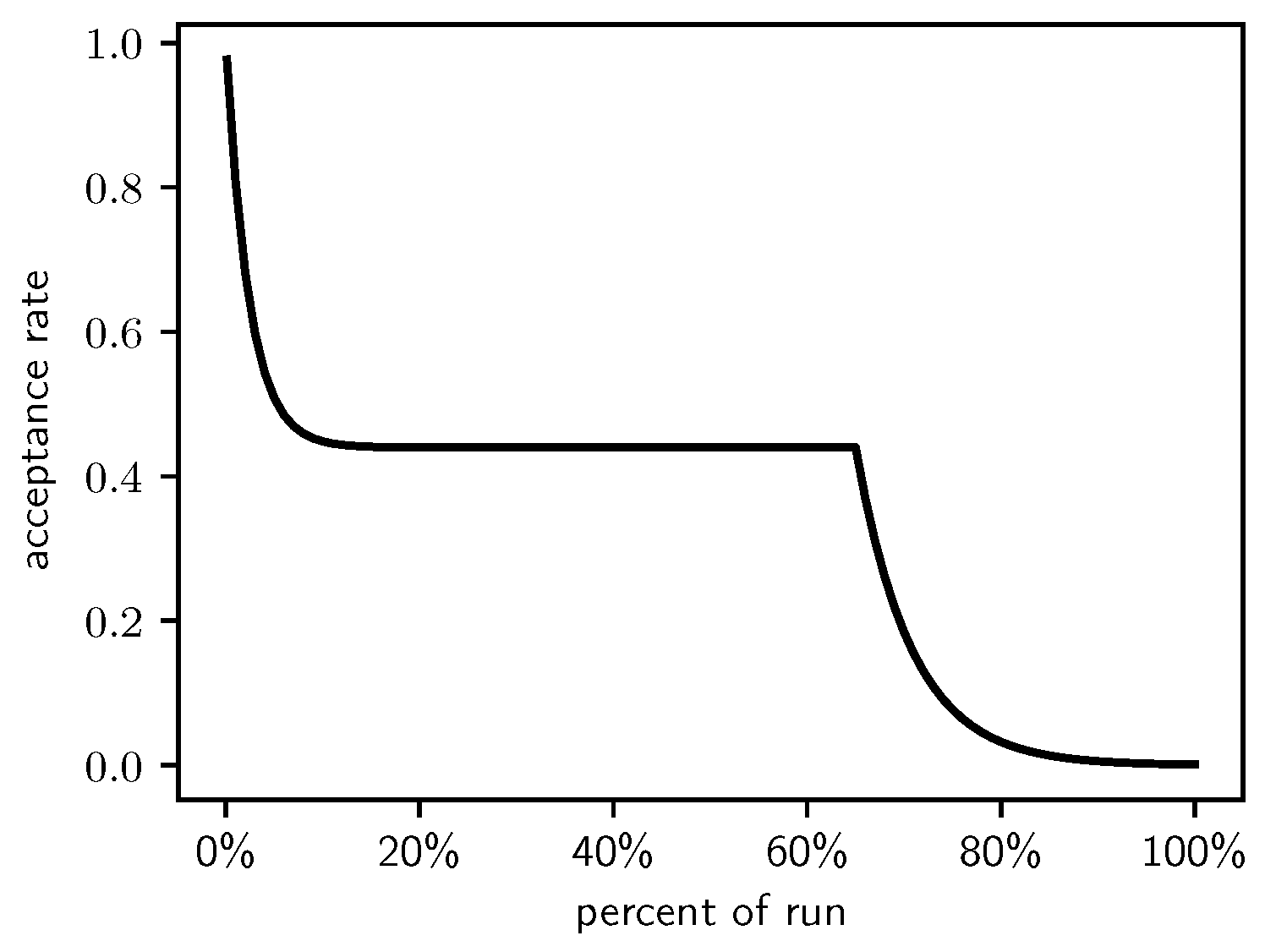
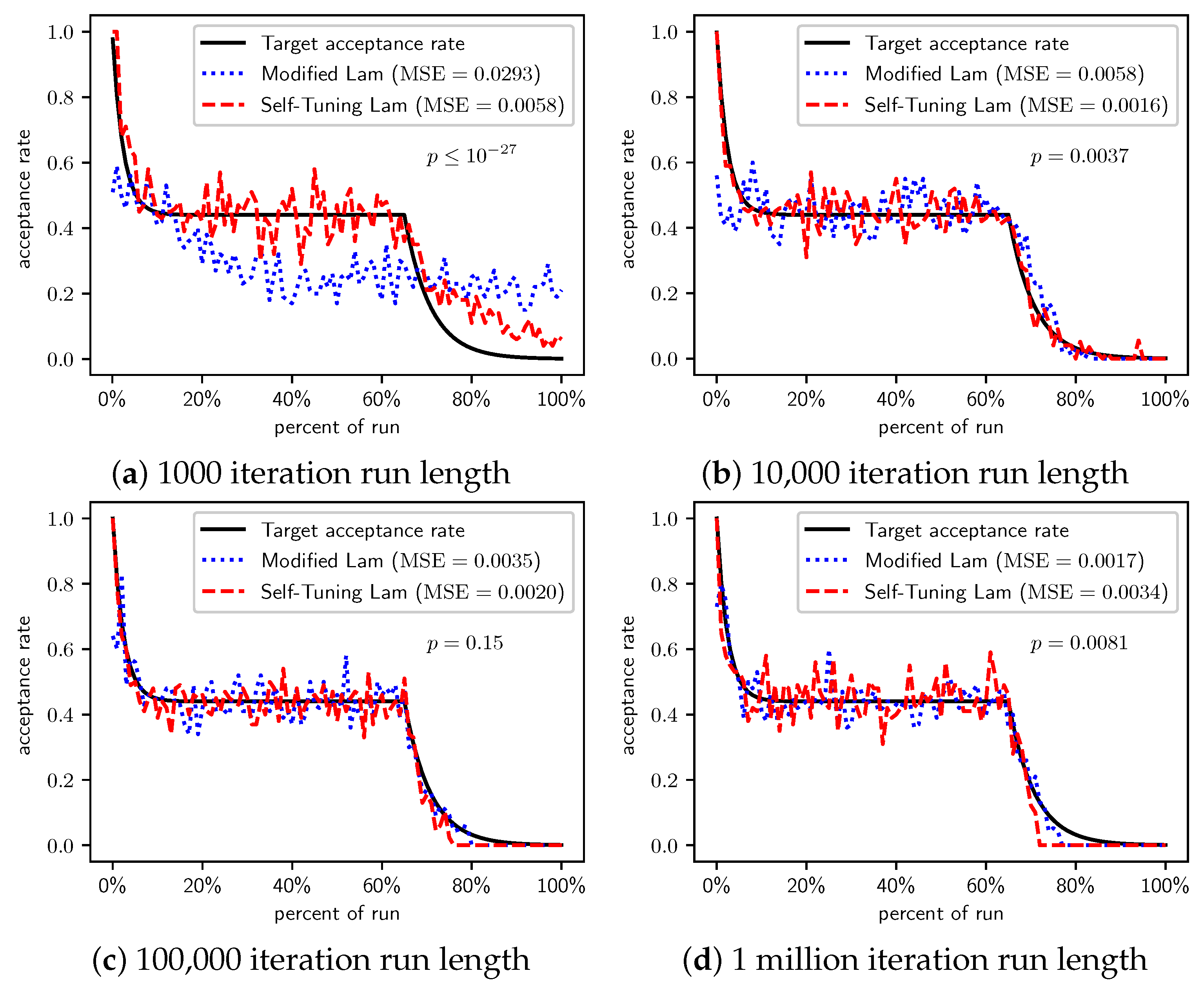
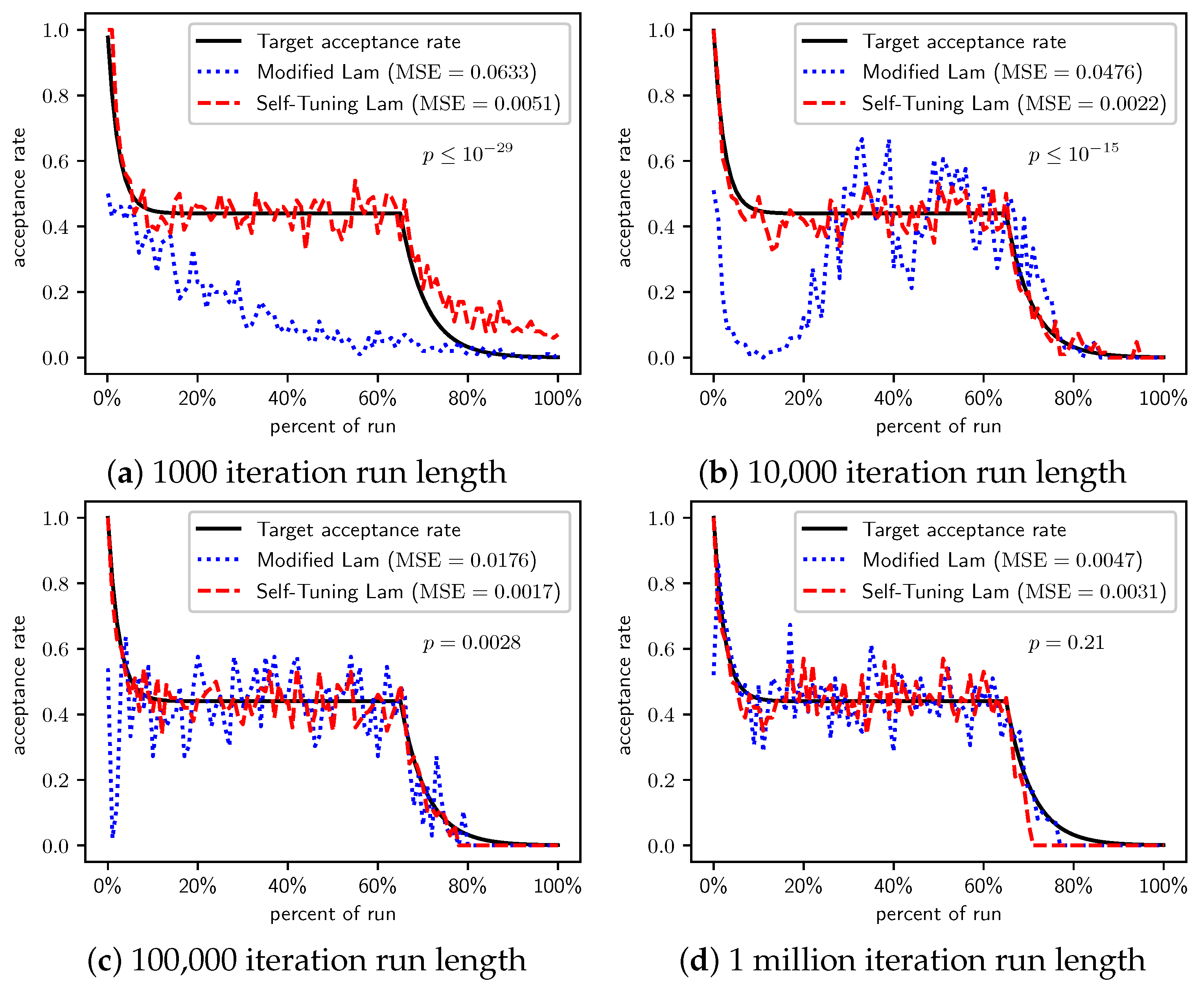
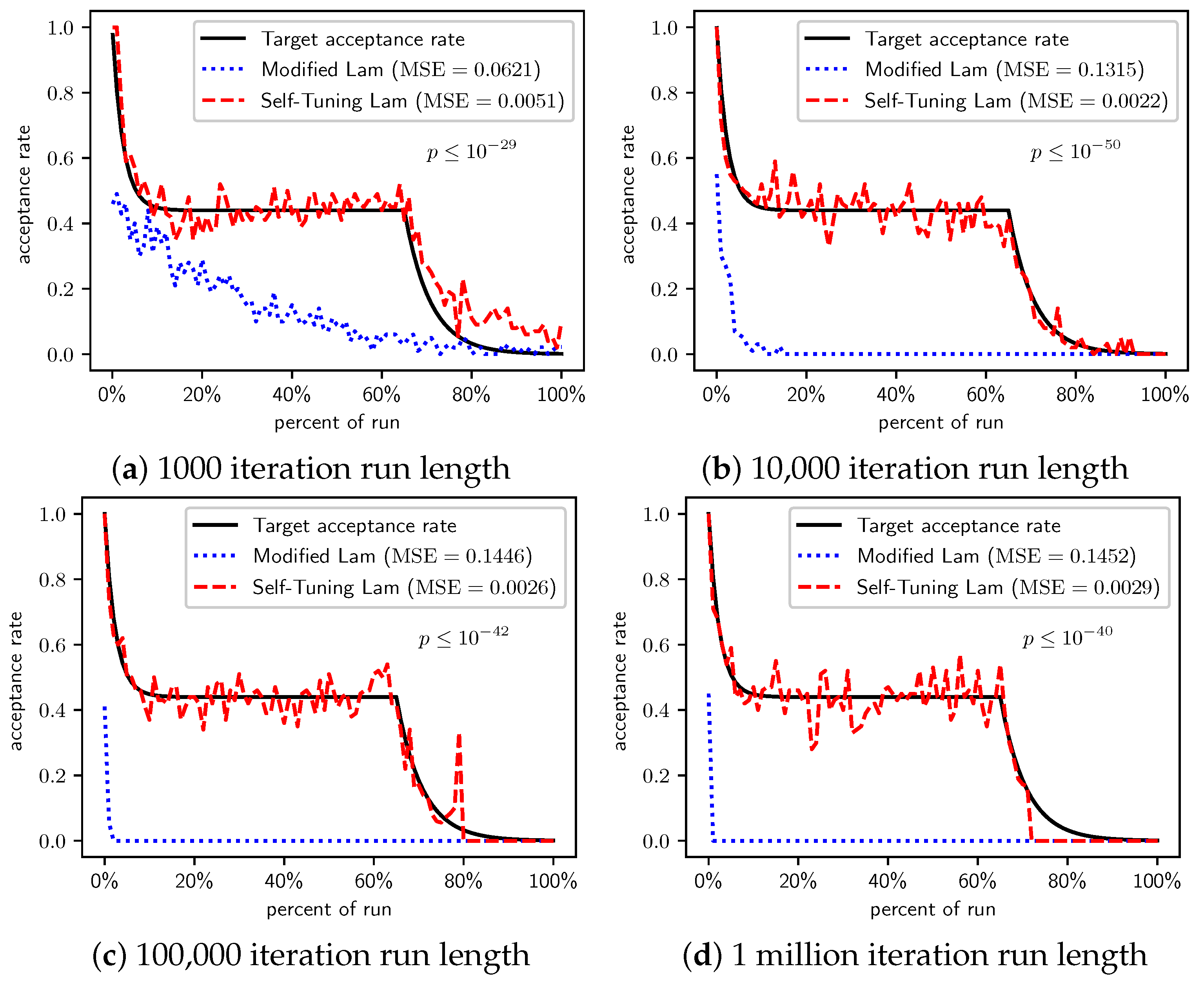
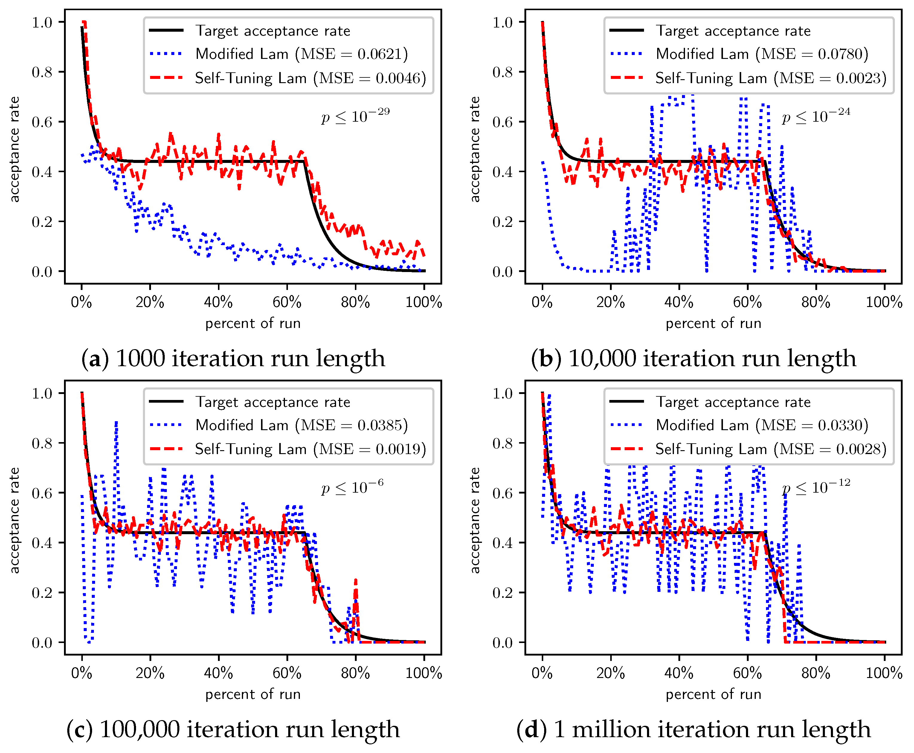
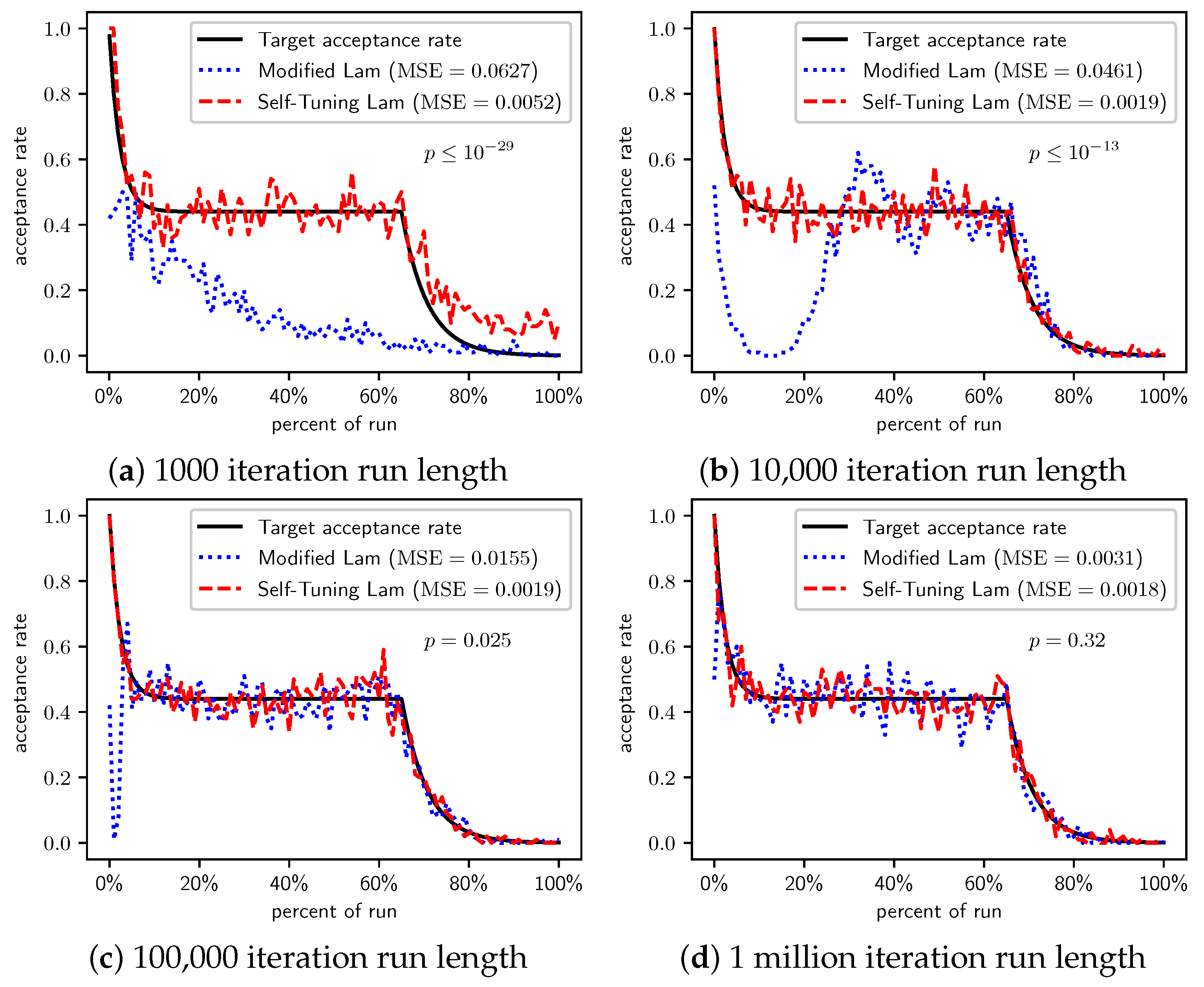
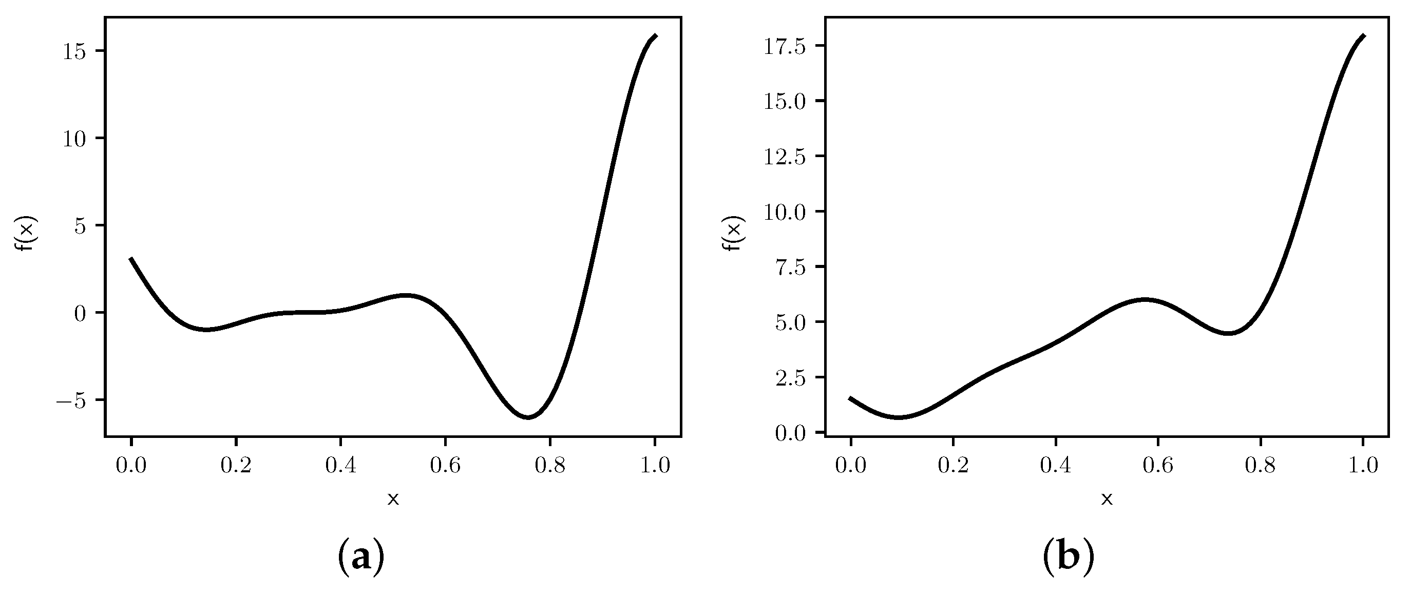
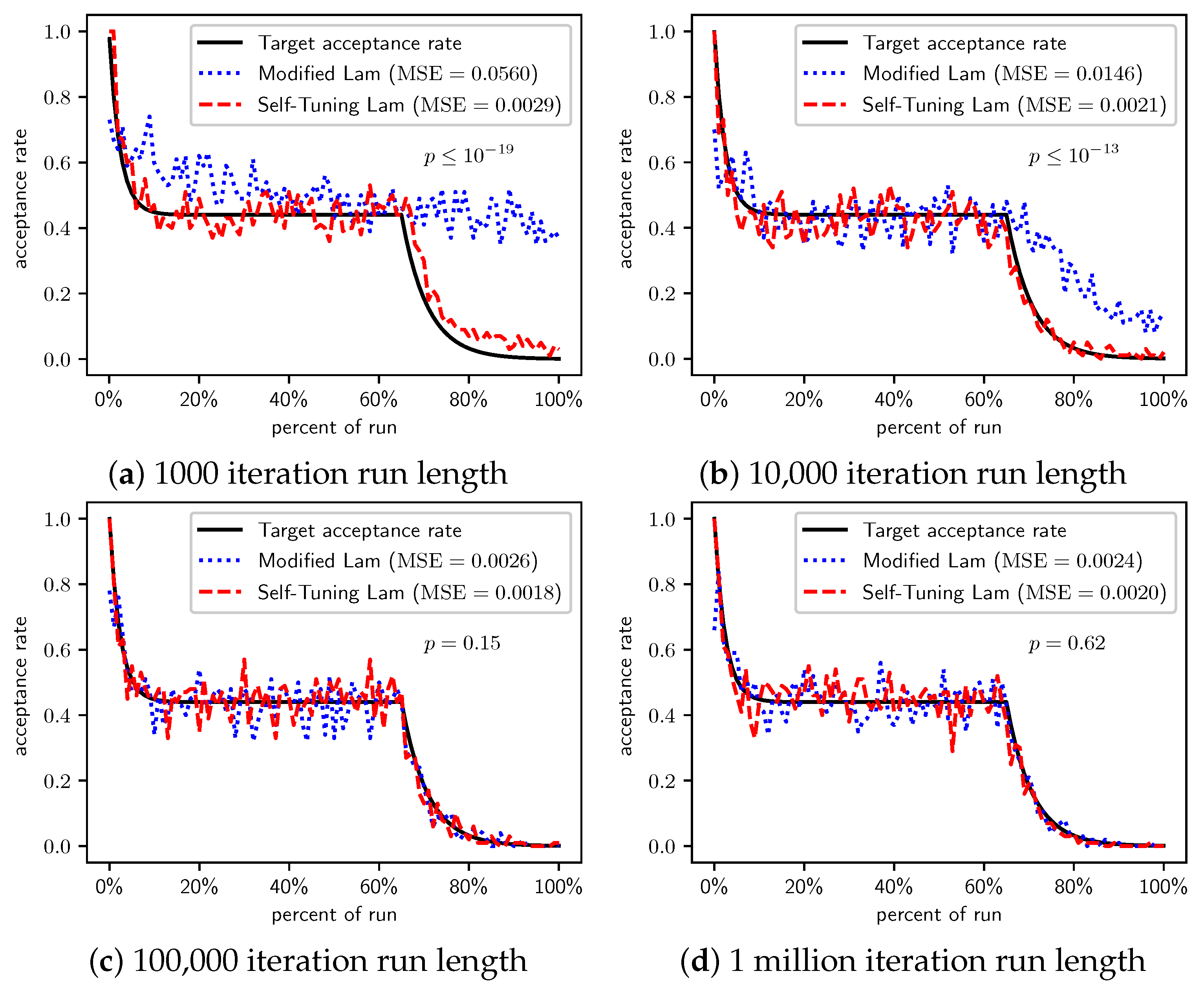
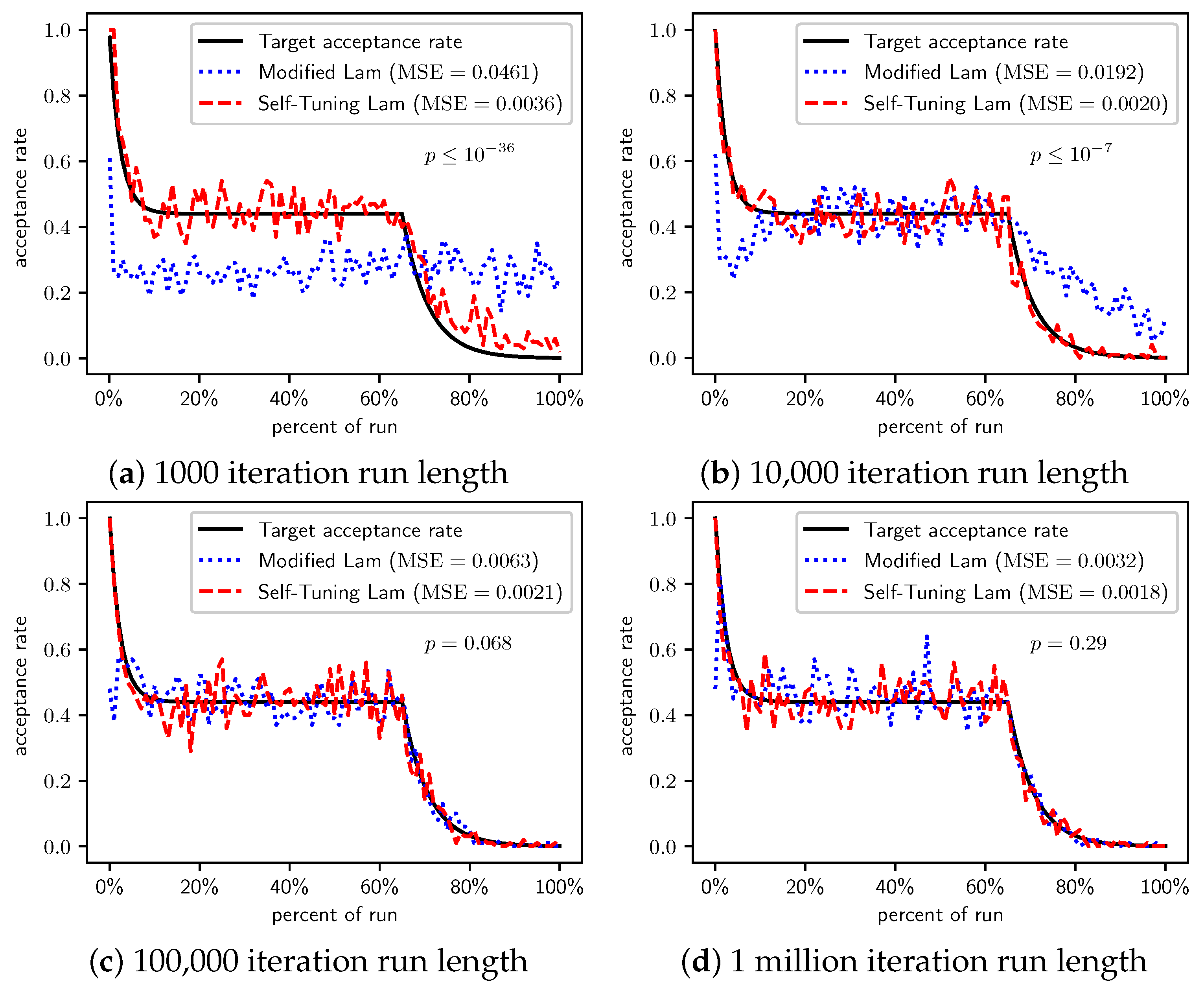
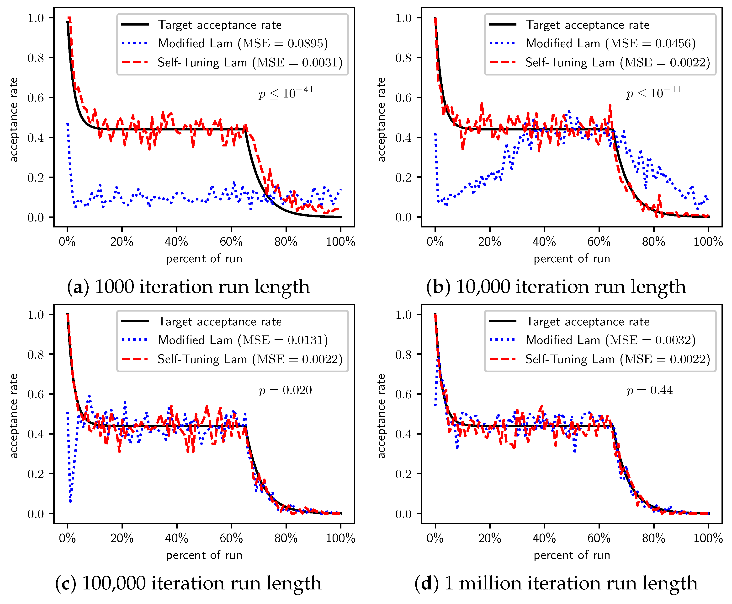
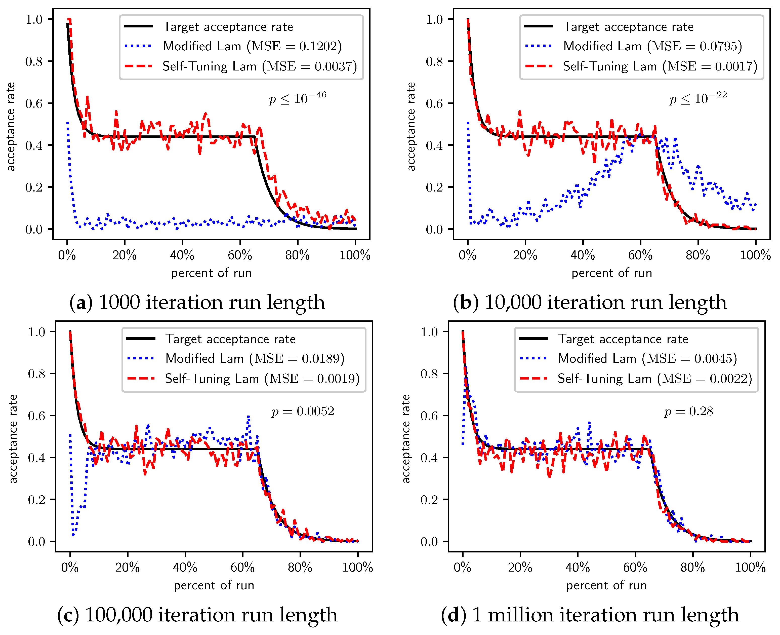
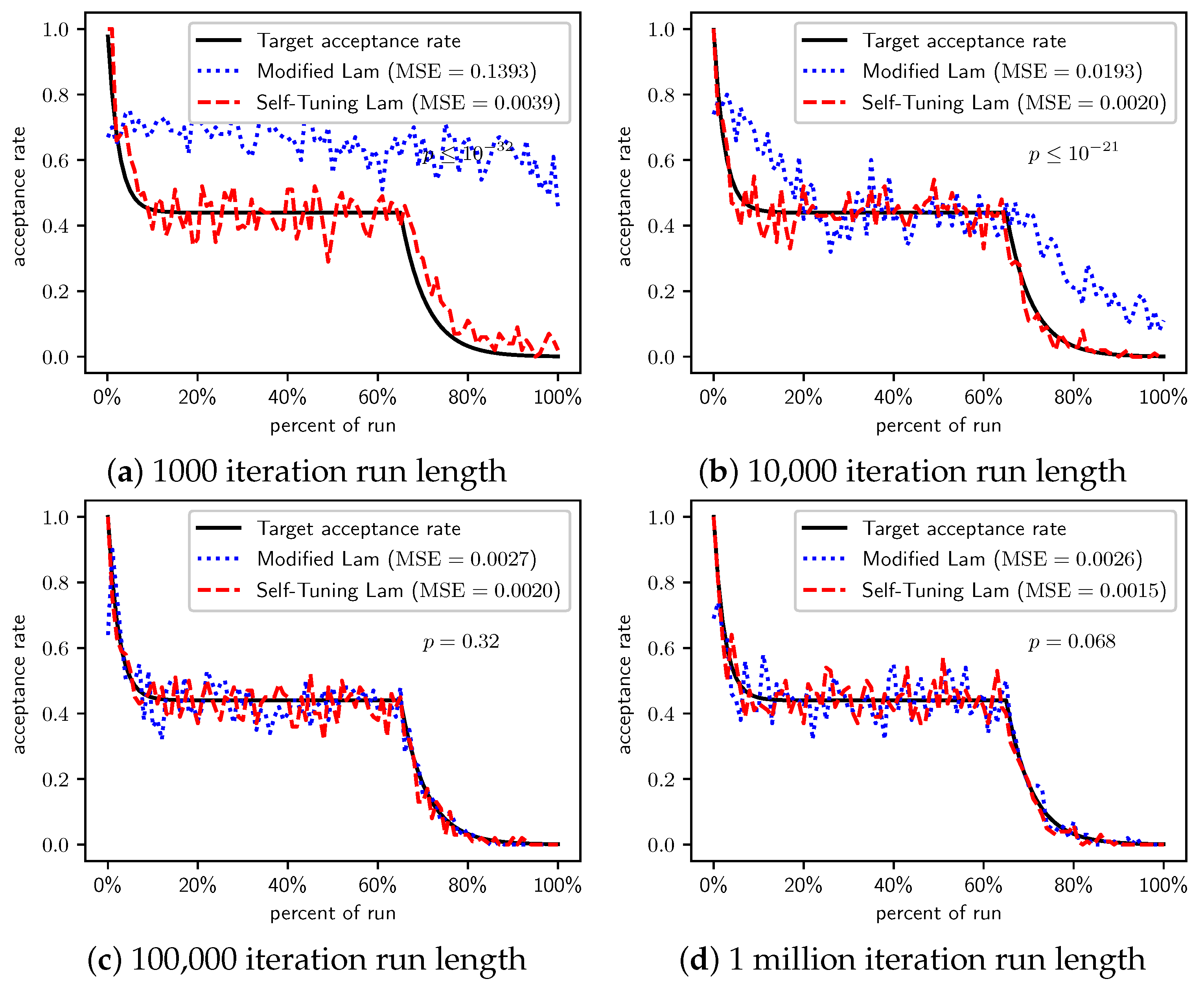
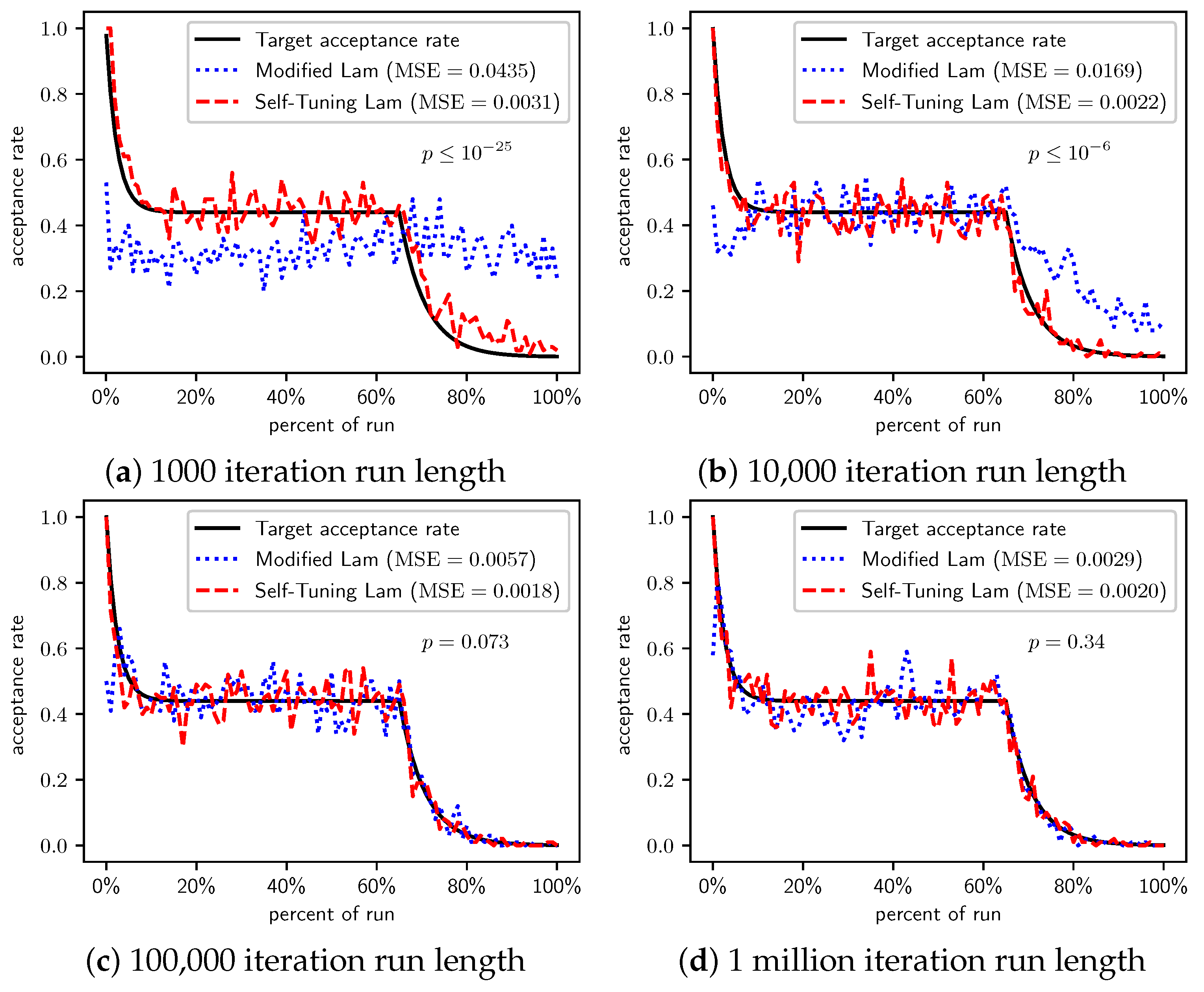
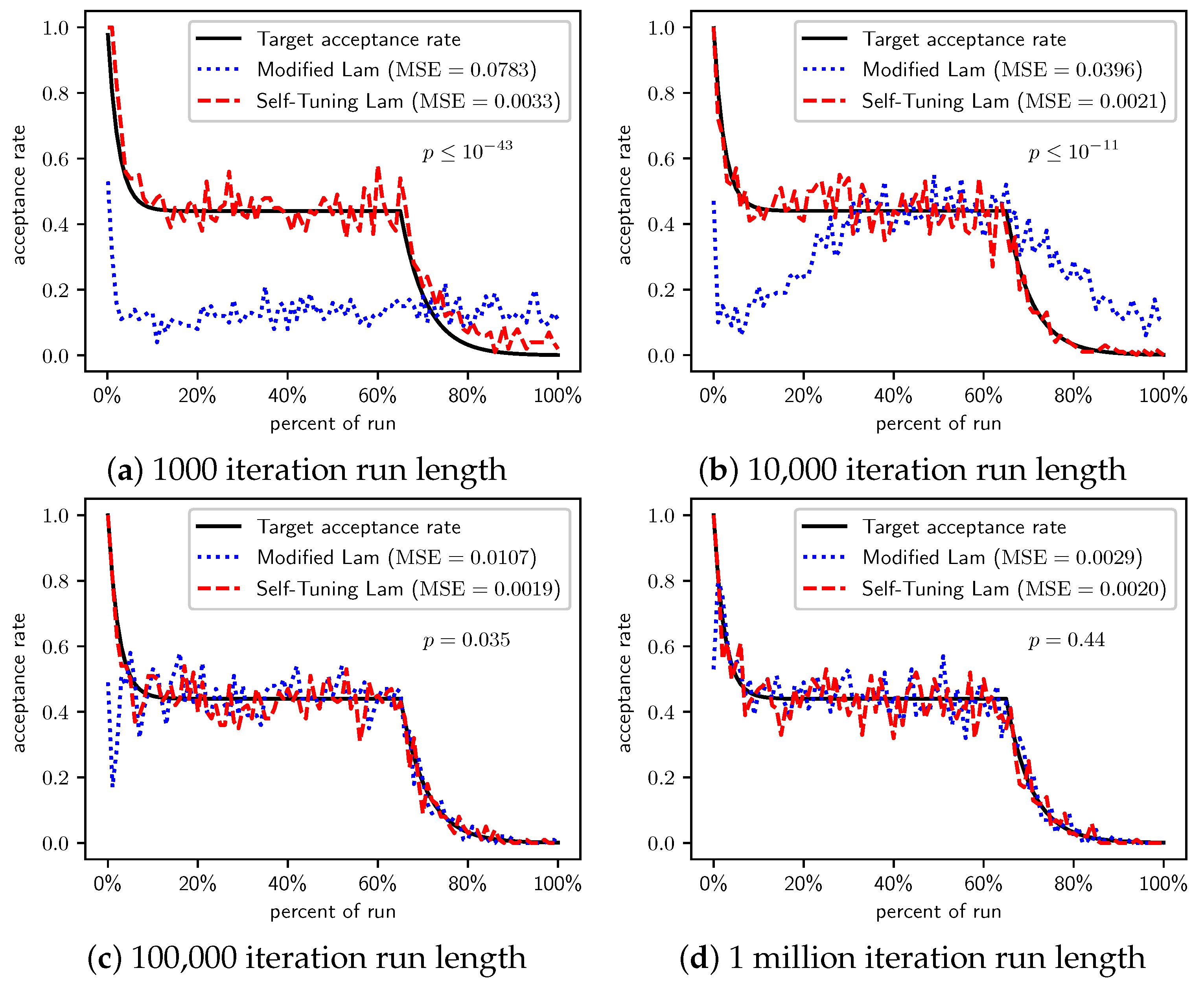
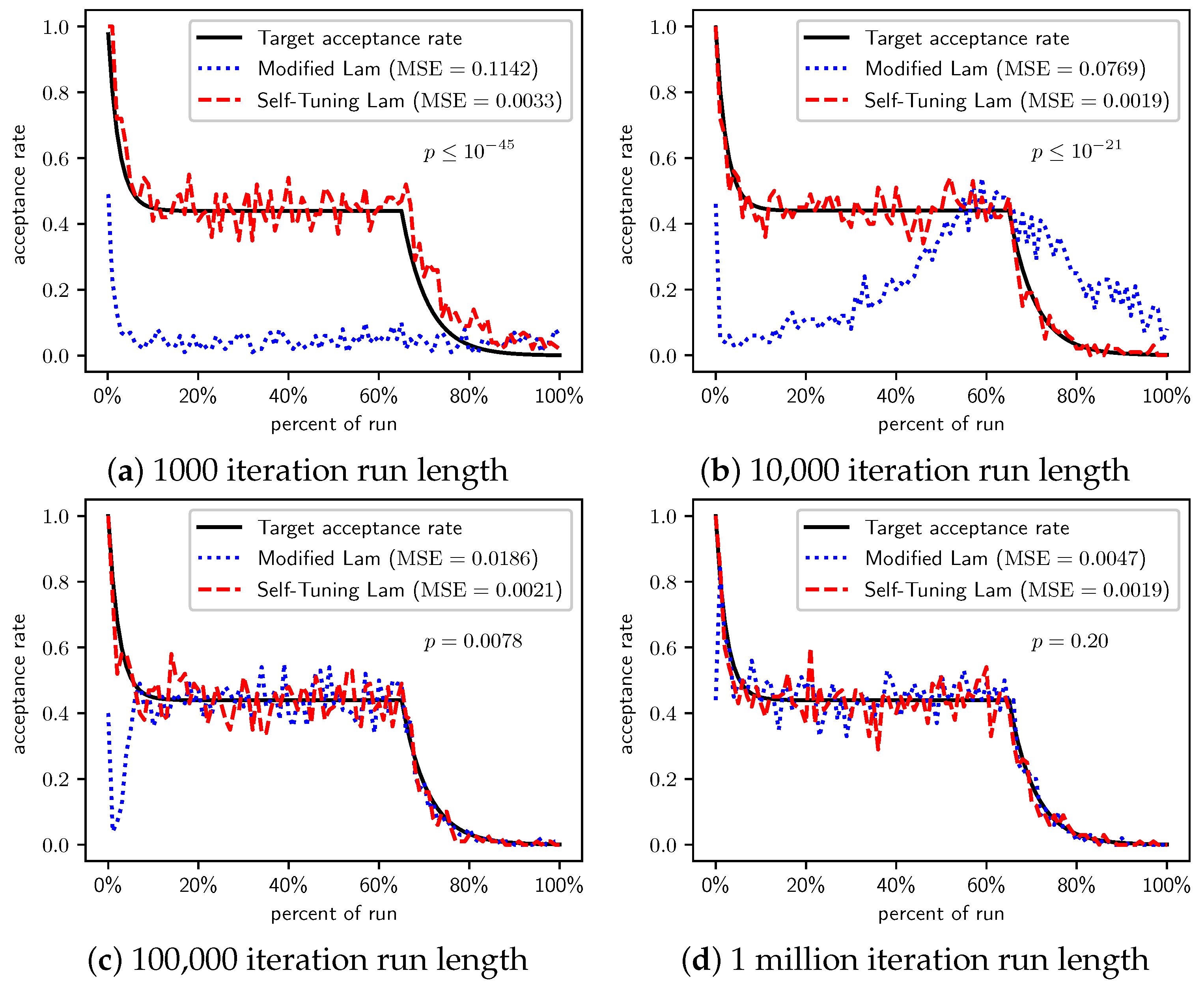
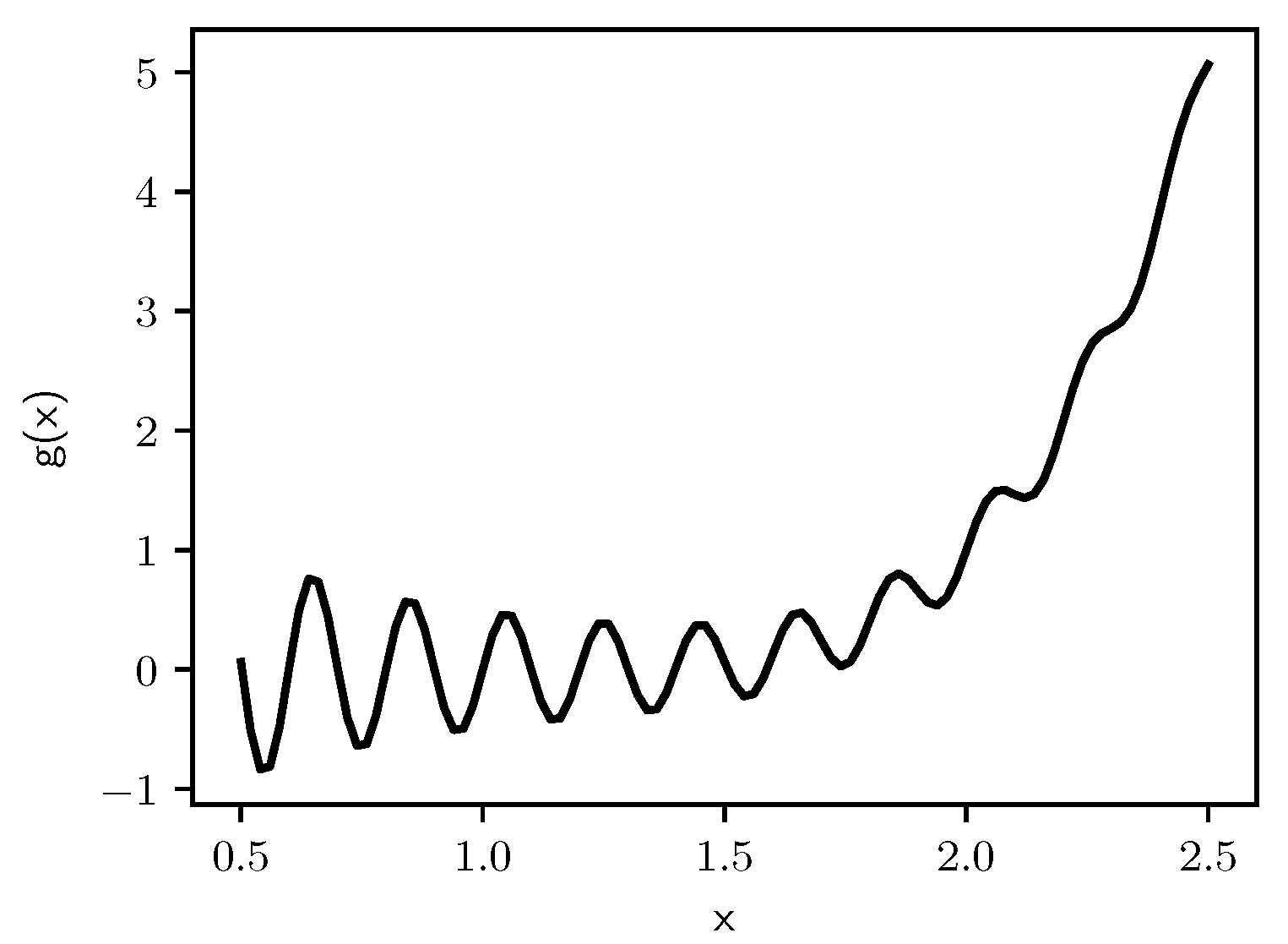
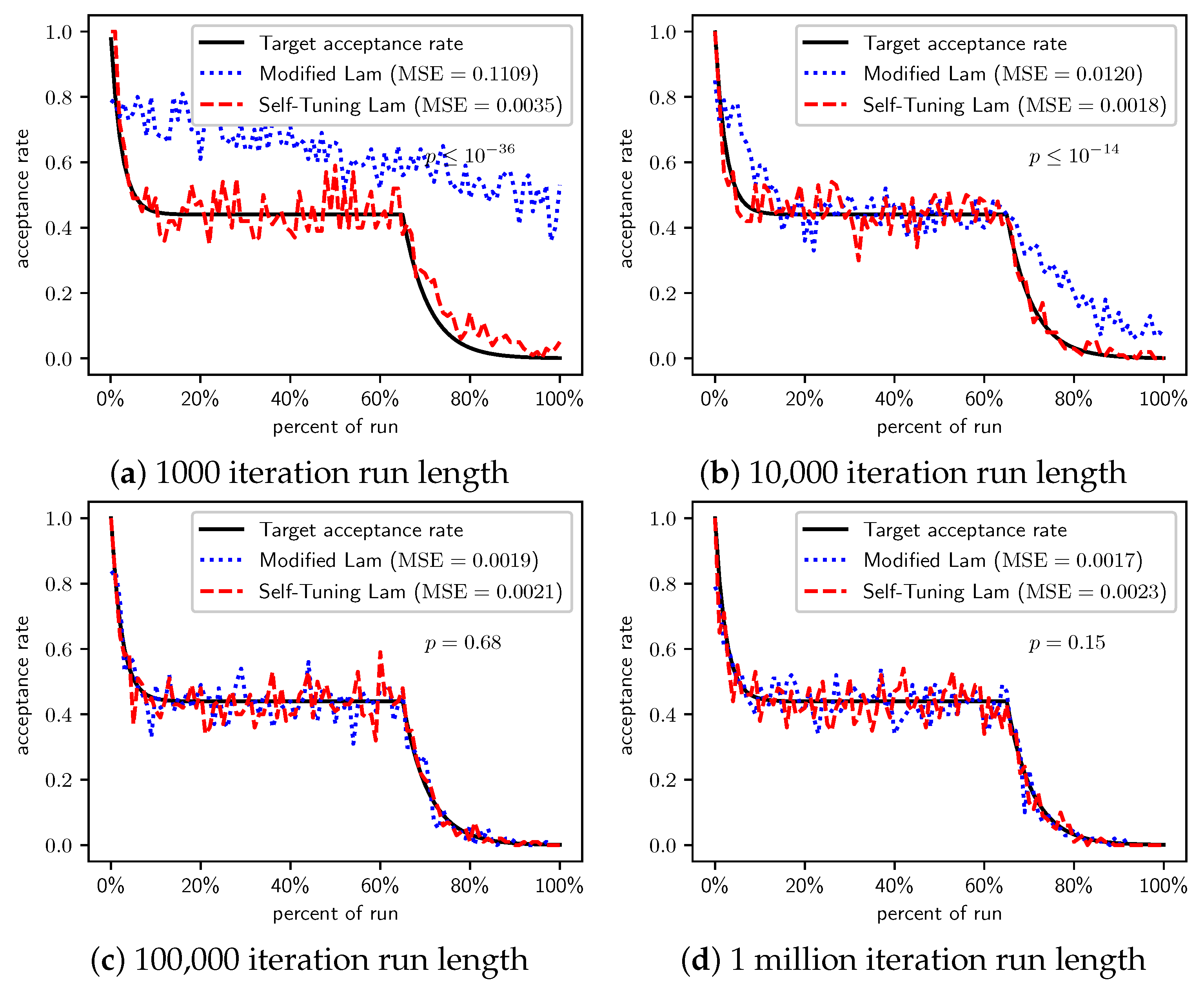
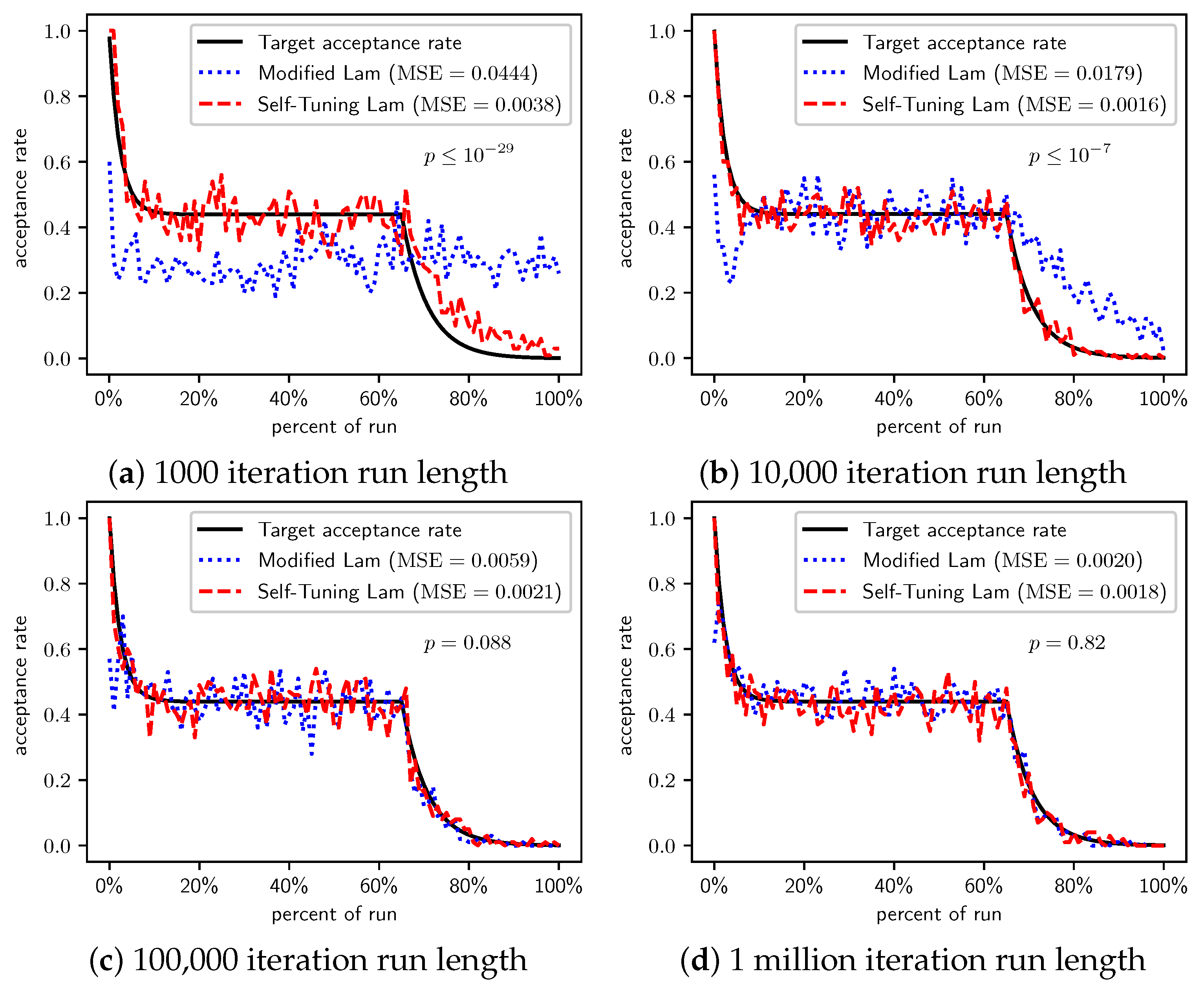
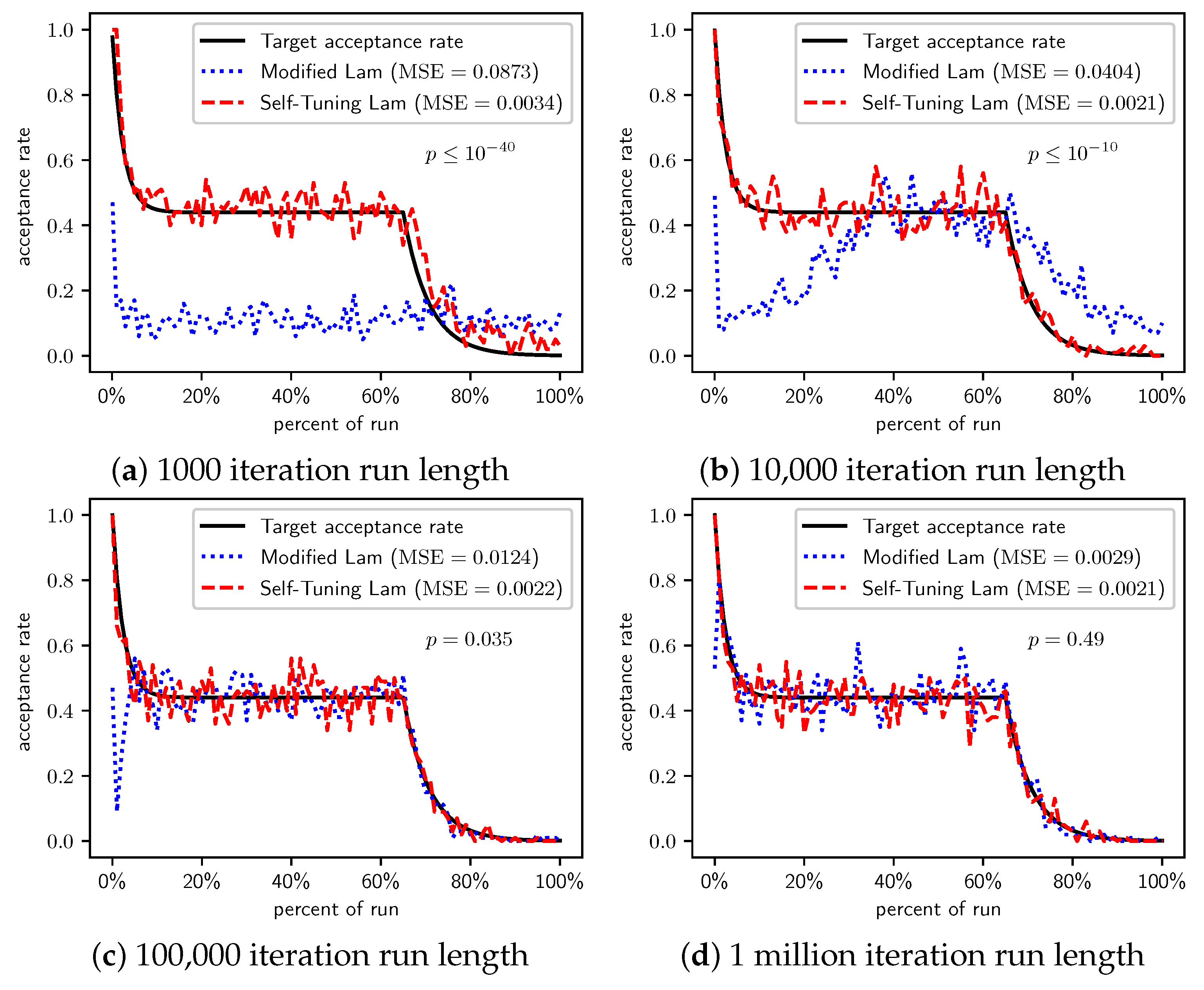
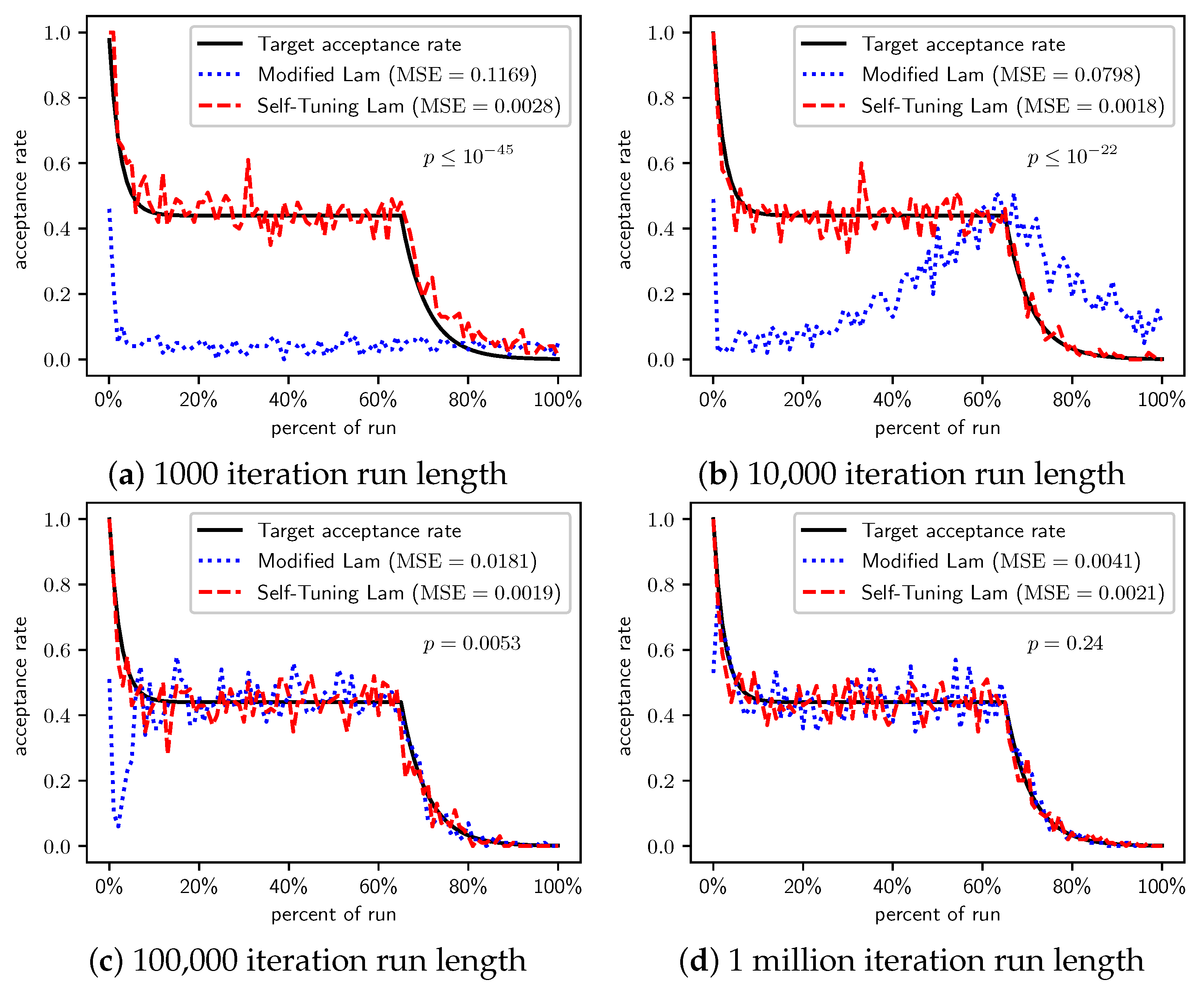
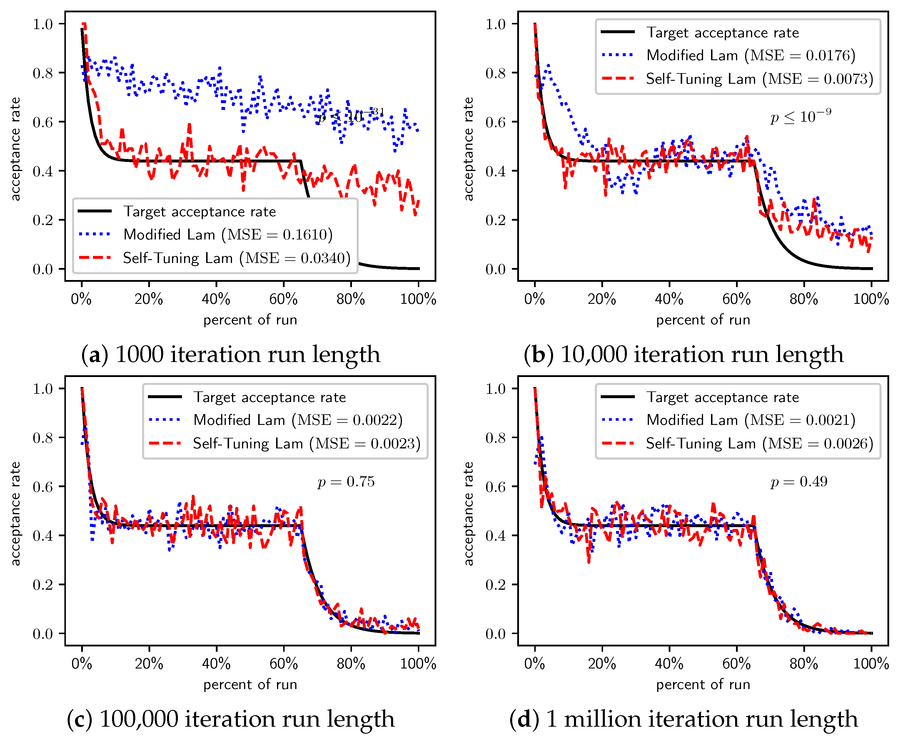
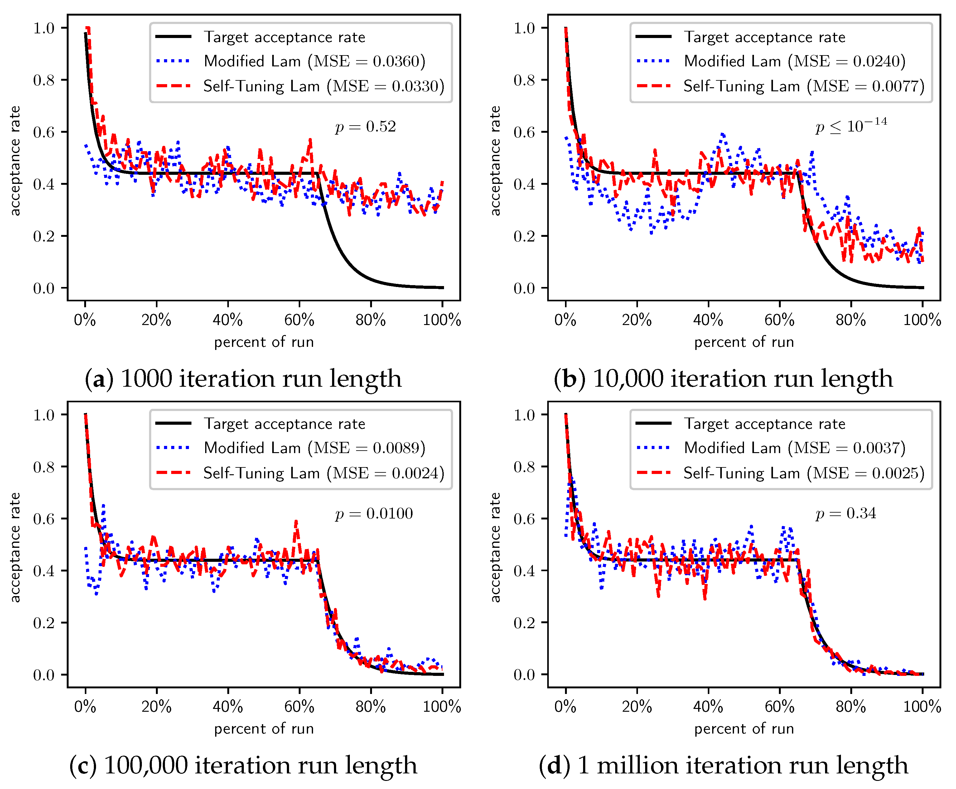
Table 1.
Constants used in the specification of the Self-Tuning Lam, including the constant, its mathematical definition, and its double-precision floating point value.
Table 1.
Constants used in the specification of the Self-Tuning Lam, including the constant, its mathematical definition, and its double-precision floating point value.
| Constant | Definition | Value |
|---|---|---|
| 0.9768670788789564 | ||
| 0.9546897506857566 | ||
| 0.8072615745900611 | ||
| 0.6808590431613767 | ||
| 0.3141120890121576 | ||
| 0.260731492877931 | ||
| 0.18987910472222955 | ||
| 0.17334743675123146 |
Table 2.
Average solution cost for the OneMax problem, case when each 0-bit costs 1.
| N | Modified Lam | Self-Tuning Lam | T-Test p-Value |
|---|---|---|---|
| 1000 | < | ||
| n/a | |||
| n/a |
Table 3.
Average solution cost for the OneMax problem, case when each 0-bit costs 10.
| N | Modified Lam | Self-Tuning Lam | T-Test p-Value |
|---|---|---|---|
| 1000 | < | ||
| n/a | |||
| n/a |
Table 4.
Average solution cost for the OneMax problem, case when each 0-bit costs 100.
| N | Modified Lam | Self-Tuning Lam | T-Test p-Value |
|---|---|---|---|
| 1000 | < | ||
| n/a | |||
| n/a |
Table 5.
Average solution cost for the TwoMax problem.
| N | Modified Lam | Self-Tuning Lam | T-Test p-Value |
|---|---|---|---|
| 1000 | < | ||
| n/a |
Table 6.
Average solution cost for the Trap problem.
| N | Modified Lam | Self-Tuning Lam | T-Test p-Value |
|---|---|---|---|
| 1000 | < | ||
| n/a | |||
| n/a |
Table 7.
Average solution for minimizing . The minimum is .
| N | Modified Lam | Self-Tuning Lam | T-Test p-Value |
|---|---|---|---|
| 1000 | |||
| n/a |
Table 8.
Average solution for minimizing . The minimum is .
| N | Modified Lam | Self-Tuning Lam | T-Test p-Value |
|---|---|---|---|
| 1000 | |||
| < | |||
| < | |||
Table 9.
Average solution for minimizing . The minimum is .
| N | Modified Lam | Self-Tuning Lam | T-Test p-Value |
|---|---|---|---|
| 1000 | |||
| < | |||
| < | |||
Table 10.
Average solution for minimizing . The minimum is .
| N | Modified Lam | Self-Tuning Lam | T-Test p-Value |
|---|---|---|---|
| 1000 | |||
| < | |||
| < | |||
Table 11.
Average solution for minimizing . The minimum is .
| N | Modified Lam | Self-Tuning Lam | T-Test p-Value |
|---|---|---|---|
| 1000 | |||
Table 12.
Average solution for minimizing . The minimum is .
| N | Modified Lam | Self-Tuning Lam | T-Test p-Value |
|---|---|---|---|
| 1000 | < | ||
| < | |||
Table 13.
Average solution for minimizing . The minimum is .
| N | Modified Lam | Self-Tuning Lam | T-Test p-Value |
|---|---|---|---|
| 1000 | |||
| < | |||
Table 14.
Average solution for minimizing . The minimum is .
| N | Modified Lam | Self-Tuning Lam | T-Test p-Value |
|---|---|---|---|
| 1000 | |||
| < | |||
Table 15.
Average solution for minimizing . The minimum is .
| N | Modified Lam | Self-Tuning Lam | T-Test p-Value |
|---|---|---|---|
| 1000 | < | ||
Table 16.
Average solution for minimizing . The minimum is .
| N | Modified Lam | Self-Tuning Lam | T-Test p-Value |
|---|---|---|---|
| 1000 | |||
Table 17.
Average solution for minimizing . The minimum is .
| N | Modified Lam | Self-Tuning Lam | T-Test p-Value |
|---|---|---|---|
| 1000 | < | ||
| < | |||
Table 18.
Average solution for minimizing . The minimum is .
| N | Modified Lam | Self-Tuning Lam | T-Test p-Value |
|---|---|---|---|
| 1000 | < | ||
| < | |||
Table 19.
Average cost of solution to TSP with 1000 cities distributed within a unit square.
| N | Modified Lam | Self-Tuning Lam | T-Test p-Value |
|---|---|---|---|
| 1000 | < | ||
| < | |||
Table 20.
Average cost of solution to TSP with 1000 cities distributed within a 100 by 100 square.
| N | Modified Lam | Self-Tuning Lam | T-Test p-Value |
|---|---|---|---|
| 1000 | |||
| < | |||
Table 21.
Runtime comparison, measured in seconds of CPU time, of the Modified Lam and Self-Tuning Lam annealing schedules. Averages of 100 runs of each run length.
Table 21.
Runtime comparison, measured in seconds of CPU time, of the Modified Lam and Self-Tuning Lam annealing schedules. Averages of 100 runs of each run length.
| N | Modified Lam | Self-Tuning Lam | T-Test p-Value |
|---|---|---|---|
Publisher’s Note: MDPI stays neutral with regard to jurisdictional claims in published maps and institutional affiliations. |
© 2021 by the author. Licensee MDPI, Basel, Switzerland. This article is an open access article distributed under the terms and conditions of the Creative Commons Attribution (CC BY) license (https://creativecommons.org/licenses/by/4.0/).
Share and Cite
MDPI and ACS Style
Cicirello, V.A. Self-Tuning Lam Annealing: Learning Hyperparameters While Problem Solving. Appl. Sci. 2021, 11, 9828. https://doi.org/10.3390/app11219828
AMA Style
Cicirello VA. Self-Tuning Lam Annealing: Learning Hyperparameters While Problem Solving. Applied Sciences. 2021; 11(21):9828. https://doi.org/10.3390/app11219828
Chicago/Turabian StyleCicirello, Vincent A. 2021. "Self-Tuning Lam Annealing: Learning Hyperparameters While Problem Solving" Applied Sciences 11, no. 21: 9828. https://doi.org/10.3390/app11219828
Note that from the first issue of 2016, this journal uses article numbers instead of page numbers. See further details here.