
Assessing Nitrate Contamination Risks in Groundwater: A Machine Learning Approach

 ,
,  , ,
, ,  , and
, and
Abstract
:1. Introduction
2. Materials and Methods
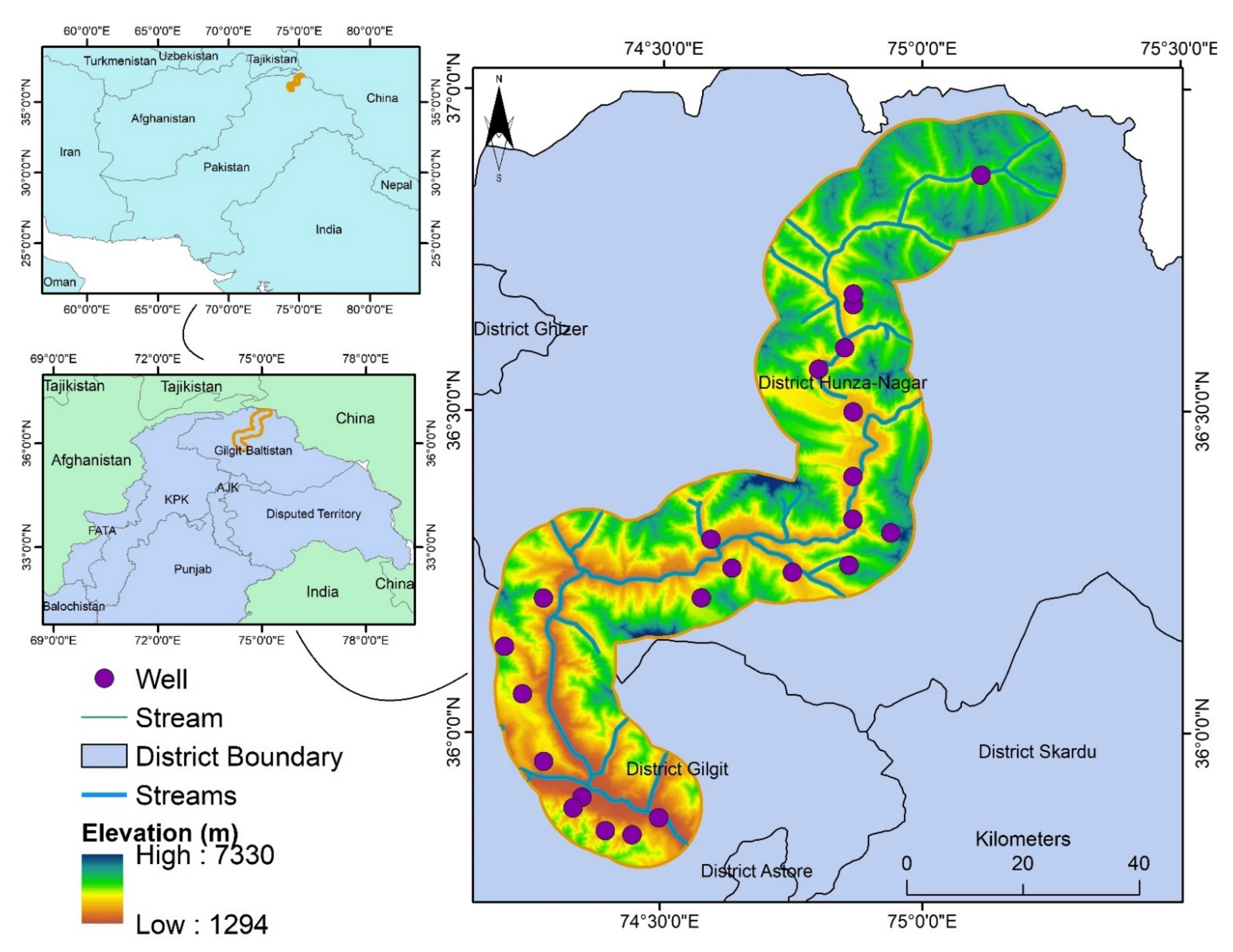
2.1. Study Area
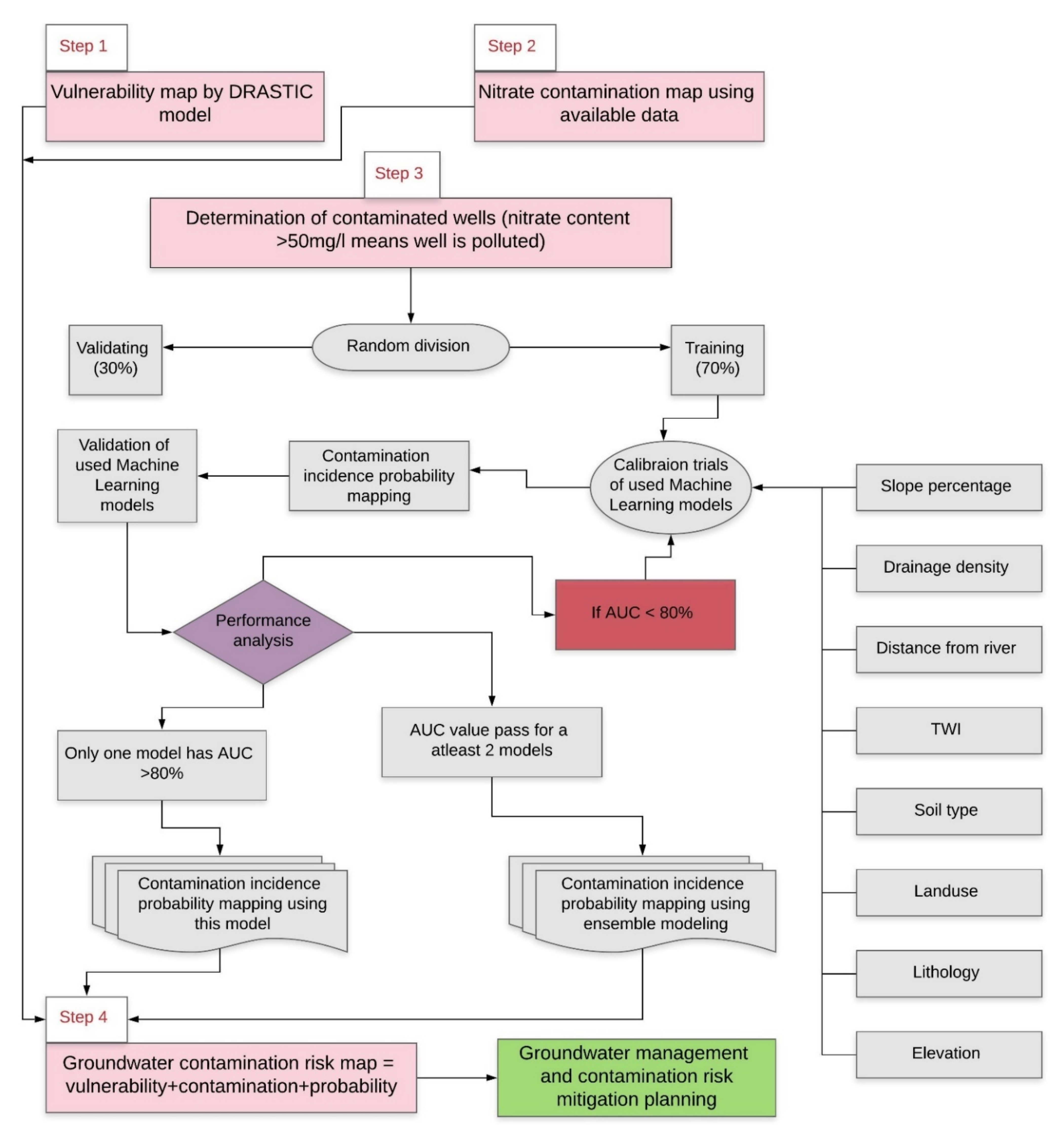
2.2. Methodology
2.3. Groundwater Vulnerability Mapping through the DRASTIC Model
2.4. Groundwater Nitrate Contamination Mapping
2.5. Groundwater Contamination Probability Mapping through Machine Learning (ML) Techniques
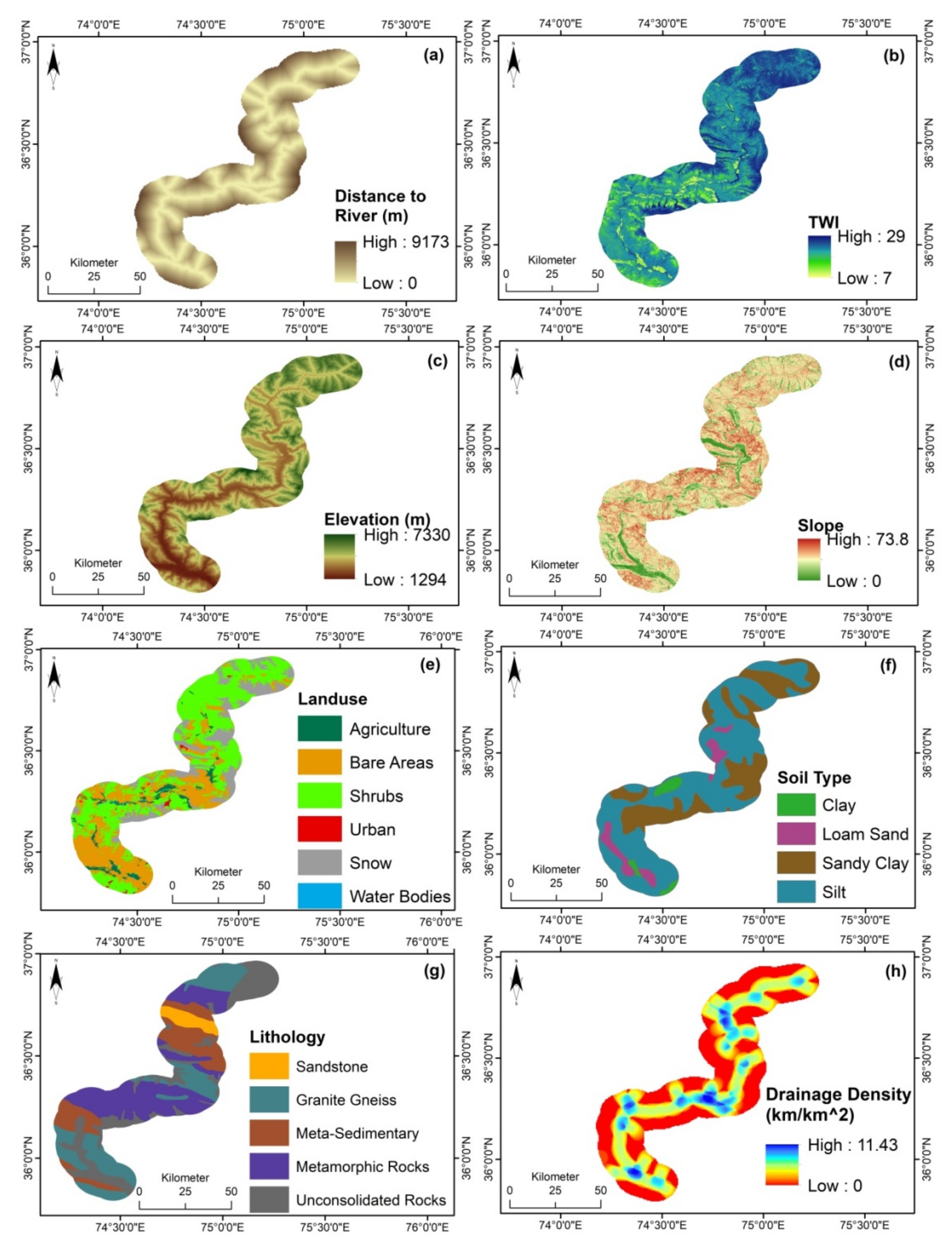
2.5.1. Groundwater Contamination Conditioning Factors
2.5.2. Boosted Regression Trees (BRT)

| Parameter | Source | Technique/Formula | Reference |
|---|---|---|---|
| Elevation | STRM DEM | 30 × 30 m DEM | [71] |
| Slope | STRM DEM | N = no. of contour cutting; i = contour interval | [72] |
| Drainage Density | STRM DEM | Proximity analysis | [73] |
| Landuse | FAO land use | Maximum likelihood | [74] |
| Distance to River | Google earth | Multiple buffer | [75] |
| TWI | STRM DEM | a = upslope contributing area (m2); b = slope in radians | [76] |
| Soil Data | Geological Maps of Pakistan | Proximity analysis | [73] |
| Lithology | Geological Maps of Pakistan | Proximity analysis | [73] |
2.5.3. Support Vector Machines (SVM)
2.5.4. Multivariate Discriminant Analysis (MDA)
2.5.5. Implementation and Accuracy Assessment
- All of the models are operated, and the accuracy is assessed. The attained AUC is measured at less than 80% for all the models. Thus, all of the models are recalibrated to achieve the threshold value (a minimum AUC value of at least 80%);
- One model achieved an AUC value over 80%, and, without further calibration, it is utilized to map the groundwater contamination incidence probability;
- All of the remaining models achieved accuracy after further recalibration trials (AUC above 80%), and are used to map the groundwater contamination incidence probability without further recalibration procedures. An ensemble modeling process was utilized, which pools the outcomes of the single models, and produces synthesized results in order to achieve further accuracy [15]. In ensemble techniques, weighted incorporation of certain models is primarily employed, such as bagging and boosting. In the present study, the following equation is used to conduct the ensemble modeling:where EM represents the Ensemble models by evaluating AUC values of each model.
2.6. Groundwater Pollution Risk Mapping
3. Results and Discussions
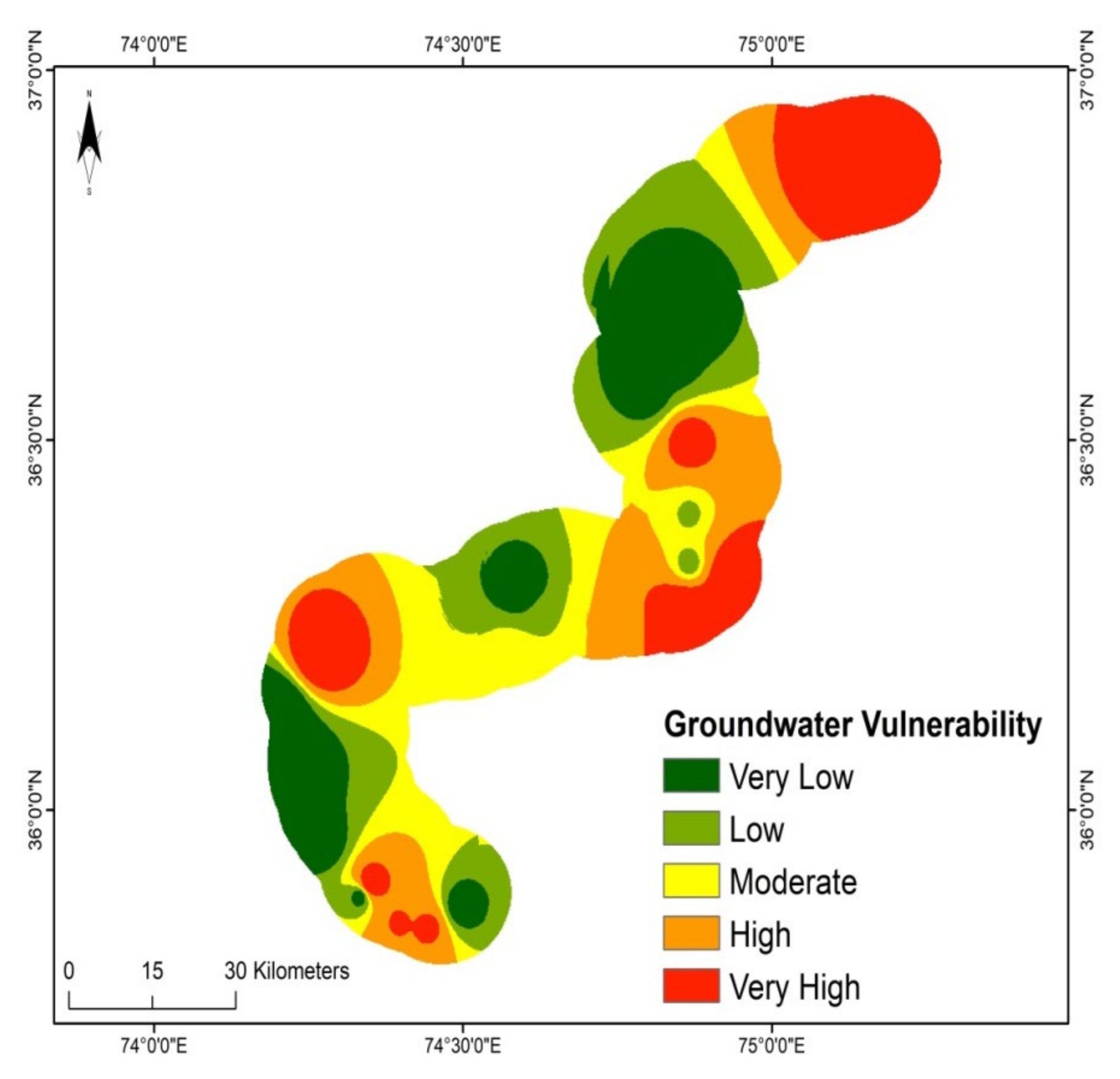
3.1. Groundwater Contamination Vulnerability Mapping
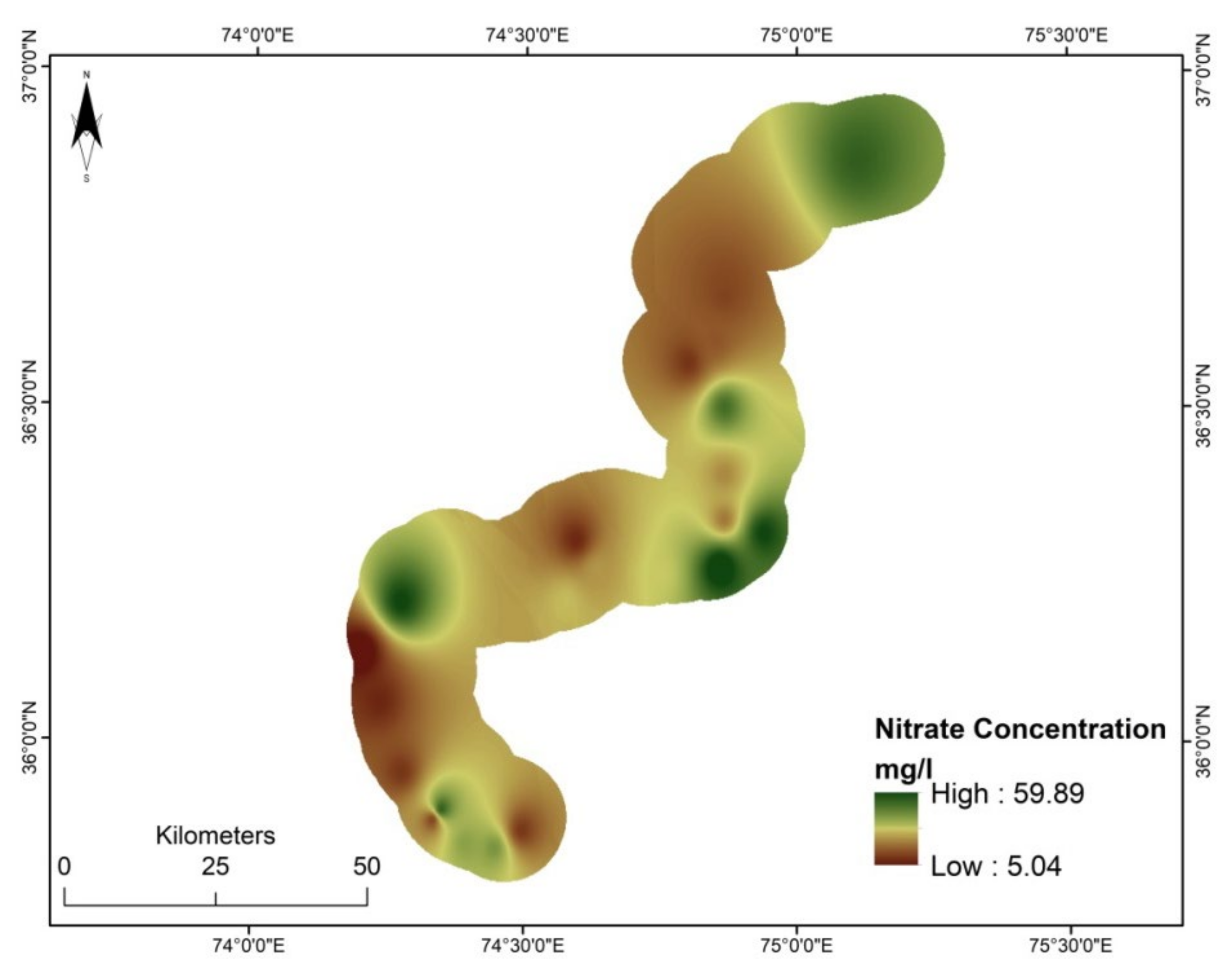
3.2. Groundwater Nitrate Concentration Mapping
3.3. Thematic Maps of Groundwater Contamination Conditioning Factors
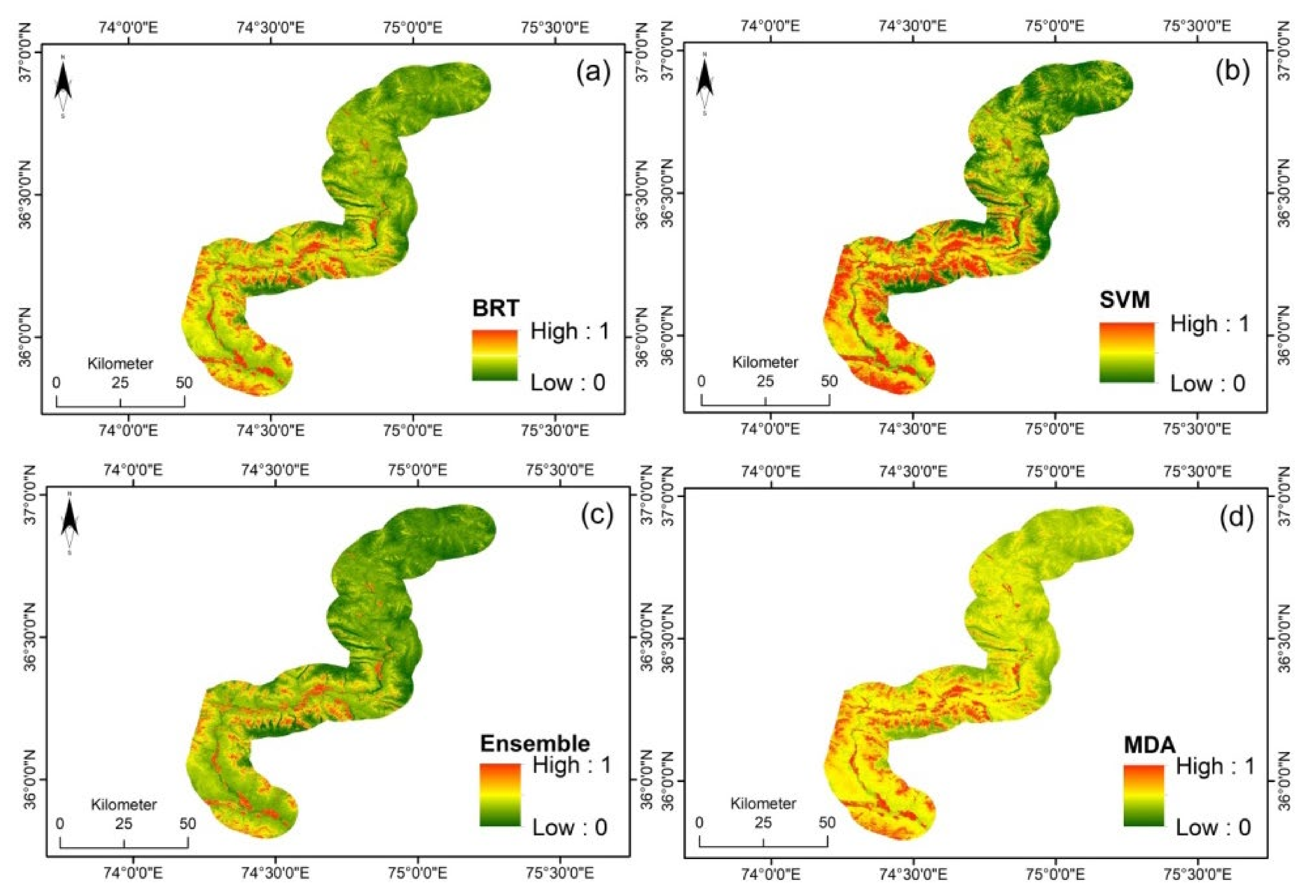
3.4. Groundwater Contamination Incidence Probability Mapping
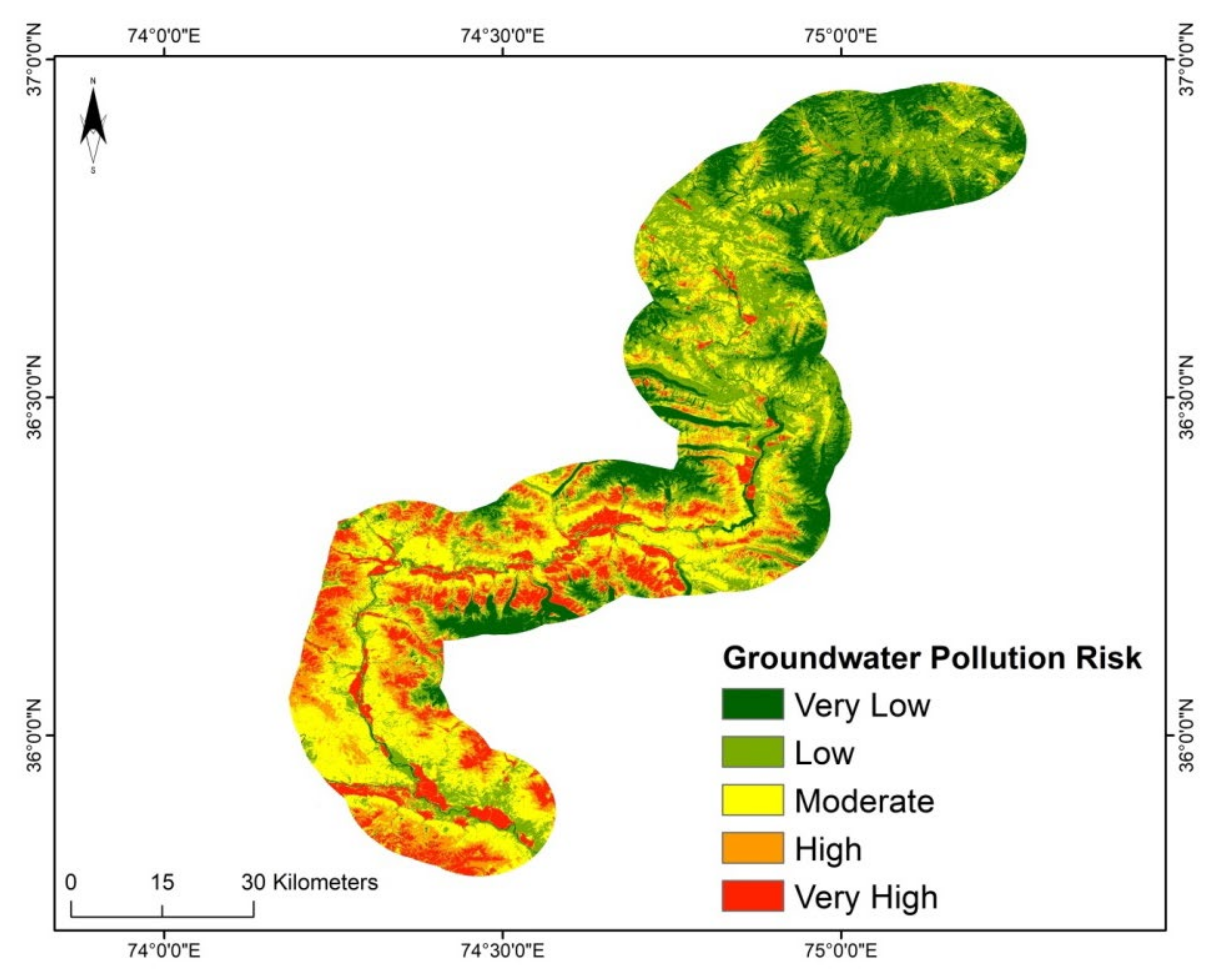
3.5. Groundwater Contamination Risk Evaluation
4. Conclusions
Author Contributions
Funding
Institutional Review Board Statement
Informed Consent Statement
Data Availability Statement
Conflicts of Interest
References
- Choubin, B.; Malekian, A.; Samadi, S.; Khalighi-Sigaroodi, S.; Hosseini, F.S. An ensemble forecast of semi-arid rainfall using large-scale climate predictors. Meteorol. Appl. 2017, 24, 376–386. [Google Scholar] [CrossRef] [Green Version]
- Neshat, A.; Pradhan, B.; Pirasteh, S.; Shafri, H.Z.M. Shafri; Estimating groundwater vulnerability to pollution using a modified DRASTIC model in the Kerman agricultural area, Iran. Environ. Earth Sci. 2014, 71, 3119–3131. [Google Scholar] [CrossRef]
- Maqsoom, A.; Aslam, B.; Khalil, U.; Ghorbanzadeh, O.; Ashraf, H.; Tufail, R.F.F.; Farooq, D.; Blaschke, T. A GIS-based DRASTIC Model and an Adjusted DRASTIC Model (DRASTICA) for Groundwater Susceptibility Assessment along the China–Pakistan Economic Corridor (CPEC) Route. ISPRS Int. J. Geo-Inf. 2020, 9, 332. [Google Scholar] [CrossRef]
- Rashid, A.; Guan, D.-X.; Farooqi, A.; Khan, S.; Zahir, S.; Jehan, S.; Khattak, S.A.; Khan, M.S.; Khan, R. Fluoride prevalence in groundwater around a fluorite mining area in the flood plain of the River Swat, Pakistan. Sci. Total Environ. 2018, 635, 203–215. [Google Scholar] [CrossRef] [Green Version]
- Hutchins, M.G.; Abesser, C.; Prudhomme, C.; Elliott, J.A.; Bloomfield, J.P.; Mansour, M.M.; Hitt, O.E. Combined impacts of future land-use and climate stressors on water resources and quality in groundwater and surface waterbodies of the upper Thames river basin, UK. Sci. Total Environ. 2018, 631, 962–986. [Google Scholar] [CrossRef]
- Hansen, B.; Thorling, L.; Schullehner, J.; Termansen, M.; Dalgaard, T. Groundwater nitrate response to sustainable nitrogen management. Sci. Rep. 2017, 7, 1–12. [Google Scholar] [CrossRef]
- Templeton, M.R.; Hammoud, A.S.; Butler, A.P.; Braun, L.; Foucher, J.-A.; Grossmann, J.; Boukari, M.; Faye, S.; Jourda, J.P. Nitrate Pollution of groundwater by pit latrines in developing countries. AIMS Environ. Sci. 2015, 2, 302. [Google Scholar] [CrossRef]
- Guo, X.; Zuo, R.; Shan, D.; Cao, Y.; Wang, J.; Teng, Y.; Fu, Q.; Zheng, B. Source apportionment of pollution in groundwater source area using factor analysis and positive matrix factorization methods. Hum. Ecol. Risk Assess. Int. J. 2017, 23, 1417–1436. [Google Scholar] [CrossRef]
- Shrestha, S.; Semkuyu, D.J.; Pandey, V.P. Assessment of groundwater vulnerability and risk to pollution in Kathmandu Valley, Nepal. Sci. Total Environ. 2016, 556, 23–35. [Google Scholar] [CrossRef]
- Ullah, F.; Sepasgozar, S.M.; Thaheem, M.J.; Wang, C.C.; Imran, M. It’s all about perceptions: A DEMATEL approach to exploring user perceptions of real estate online platforms. Ain Shams Eng. J. 2021. [Google Scholar] [CrossRef]
- Ullah, F.; Sepasgozar, S.M.; Shirowzhan, S.; Davis, S. Modelling users’ perception of the online real estate platforms in a digitally disruptive environment: An integrated KANO-SISQual approach. Telemat. Inform. 2021, 63, 101660. [Google Scholar] [CrossRef]
- Ullah, F. A beginner’s guide to developing review-based conceptual frameworks in the built environment. Architecture 2021, 1, 3. [Google Scholar] [CrossRef]
- Munawar, H.S.; Ullah, F.; Qayyum, S.; Heravi, A. Application of Deep Learning on UAV-Based Aerial Images for Flood Detection. Smart Cities 2021, 4, 65. [Google Scholar] [CrossRef]
- Hussain, Y.; Satgé, F.; Hussain, M.B.; Martinez-Carvajal, H.; Bonnet, M.-P.; Cárdenas-Soto, M.; Roig, H.L.; Akhter, G. Performance of CMORPH, TMPA, and PERSIANN rainfall datasets over plain, mountainous, and glacial regions of Pakistan. Theor. Appl. Climatol. 2018, 131, 1119–1132. [Google Scholar] [CrossRef]
- Sajedi-Hosseini, F.; Malekian, A.; Choubin, B.; Rahmati, O.; Cipullo, S.; Coulon, F.; Pradhan, B. A novel machine learning-based approach for the risk assessment of nitrate groundwater contamination. Sci. Total Environ. 2018, 644, 954–962. [Google Scholar] [CrossRef] [Green Version]
- Rashid, A.; Farooqi, A.; Gao, X.; Zahir, S.; Noor, S.; Khattak, J.A. Geochemical modeling, source apportionment, health risk exposure and control of higher fluoride in groundwater of sub-district Dargai, Pakistan. Chemosphere 2020, 243, 125409. [Google Scholar] [CrossRef]
- Zafar, M.; Ahmad, W. Water quality assessment and apportionment of northern Pakistan by multivariate statistical techniques, a case study. Int. J. Hydro. 2018, 2, 00040. [Google Scholar]
- Somaratne, N.; Zulfic, H.; Ashman, G.; Vial, H.; Swaffer, B.; Frizenschaf, J. Groundwater risk assessment model (GRAM): Groundwater risk assessment model for wellfield protection. Water 2013, 5, 1419–1439. [Google Scholar] [CrossRef] [Green Version]
- Foster, S.; Hirata, R.; Andreo, B. The aquifer pollution vulnerability concept: Aid or impediment in promoting groundwater protection? Hydrogeol. J. 2013, 21, 1389–1392. [Google Scholar] [CrossRef]
- Vrba, J.; Zaporozec, A. Guidebook on Mapping Groundwater Vulnerability; Heise: Hanover, Germany, 1994. [Google Scholar]
- Gogu, R.C.; Dassargues, A. Current trends and future challenges in groundwater vulnerability assessment using overlay and index methods. Environ. Geol. 2000, 39, 549–559. [Google Scholar] [CrossRef]
- Zhou, J.; Li, G.; Liu, F.; Wang, Y.; Guo, X. DRAV model and its application in assessing groundwater vulnerability in arid area: A case study of pore phreatic water in Tarim Basin, Xinjiang, Northwest China. Environ. Earth Sci. 2010, 60, 1055–1063. [Google Scholar] [CrossRef]
- Van Beynen, P.; Niedzielski, M.; Bialkowska-Jelinska, E.; Alsharif, K.; Matusick, J. Comparative study of specific groundwater vulnerability of a karst aquifer in central Florida. Appl. Geogr. 2012, 32, 868–877. [Google Scholar] [CrossRef]
- Foster, S. Fundamental Concepts in Aquifer Vulnerability, Pollution Risk and Protection Strategy; Netherlands Organization for Applied Scientific Research: The Hague, The Netherlands, 1987. [Google Scholar]
- De Filippis, G.; Ercoli, L.; Rossetto, R. A Spatially Distributed, Physically-Based Modeling Approach for Estimating Agricultural Nitrate Leaching to Groundwater. Hydrology 2021, 8, 8. [Google Scholar] [CrossRef]
- Narany, T.S.; Ramli, M.F.; Sulaiman, W.N.A.; Fakharian, K. Assessment of the Potential Contamination Risk of Nitrate in Groundwater Using Indicator Kriging (in Amol–Babol Plain, Iran). In From Sources to Solution; Springer: Berlin/Heidelberg, Germany, 2014; pp. 273–277. [Google Scholar]
- Stigter, T.Y.; Ribeiro, L.; Dill, A.C. Evaluation of an intrinsic and a specific vulnerability assessment method in comparison with groundwater salinisation and nitrate contamination levels in two agricultural regions in the south of Portugal. Hydrogeol. J. 2006, 14, 79–99. [Google Scholar] [CrossRef]
- Gong, G.; Mattevada, S.; O’Bryant, S. Comparison of the accuracy of kriging and IDW interpolations in estimating groundwater arsenic concentrations in Texas. Environ. Res. 2014, 130, 59–69. [Google Scholar] [CrossRef] [PubMed]
- Kaown, D.; Hyun, Y.; Bae, G.-O.; Lee, K.-K. Factors affecting the spatial pattern of nitrate contamination in shallow groundwater. J. Environ. Qual. 2007, 36, 1479–1487. [Google Scholar] [CrossRef] [PubMed]
- Akbar, T.A.; Lin, H.; DeGroote, J. Development and evaluation of GIS-based ArcPRZM-3 system for spatial modeling of groundwater vulnerability to pesticide contamination. Comput. Geosci. 2011, 37, 822–830. [Google Scholar] [CrossRef]
- Fontaine, D.D.; Havens, P.L.; Blau, G.E.; Tillotson, P.M. The role of sensitivity analysis in groundwater risk modeling for pesticides. Weed Technol. 1992, 6, 716–724. [Google Scholar] [CrossRef]
- Leonard, R.A.; Knisel, W.G.; Still, D.A. GLEAMS: Groundwater loading effects of agricultural management systems. Trans. ASAE 1987, 30, 1403–1418. [Google Scholar] [CrossRef]
- Leone, A.; Ripa, M.N.; Uricchio, V.; Deak, J.; Vargay, Z. Vulnerability and risk evaluation of agricultural nitrogen pollution for Hungary’s main aquifer using DRASTIC and GLEAMS models. J. Environ. Manag. 2009, 90, 2969–2978. [Google Scholar] [CrossRef]
- Bonton, A.; Rouleau, A.; Bouchard, C.; Rodríguez, M.J. Nitrate transport modeling to evaluate source water protection scenarios for a municipal well in an agricultural area. Agric. Syst. 2011, 104, 429–439. [Google Scholar] [CrossRef]
- Qin, R.; Wu, Y.; Xu, Z.; Xie, D.; Zhang, C. Assessing the impact of natural and anthropogenic activities on groundwater quality in coastal alluvial aquifers of the lower Liaohe River Plain, NE China. Appl. Geochem. 2013, 31, 142–158. [Google Scholar] [CrossRef]
- Nobre, R.; Filho, O.R.; Mansur, W.; Nobre, M.; Cosenza, C. Groundwater vulnerability and risk mapping using GIS, modeling and a fuzzy logic tool. J. Contam. Hydrol. 2007, 94, 277–292. [Google Scholar] [CrossRef] [PubMed]
- Iqbal, J.; Gorai, A.K.; Tirkey, P.; Pathak, G. Approaches to groundwater vulnerability to pollution: A literature review. Asian J. Water Environ. Pollut. 2012, 9, 105–115. [Google Scholar]
- Anane, M.; Abidi, B.; Lachaal, F.; Limam, A.; Jellali, S. GIS-based DRASTIC, Pesticide DRASTIC and the Susceptibility Index (SI): Comparative study for evaluation of pollution potential in the Nabeul-Hammamet shallow aquifer, Tunisia. Hydrogeol. J. 2013, 21, 715–731. [Google Scholar] [CrossRef]
- Garnier, M.; Porto, A.L.; Marini, R.; Leone, A. Integrated use of GLEAMS and GIS to prevent groundwater pollution caused by agricultural disposal of animal waste. Environ. Manag. 1998, 22, 747–756. [Google Scholar] [CrossRef] [PubMed]
- Johnson, T.D.; Belitz, K. Assigning land use to supply wells for the statistical characterization of regional groundwater quality: Correlating urban land use and VOC occurrence. J. Hydrol. 2009, 370, 100–108. [Google Scholar] [CrossRef]
- McLay, C.; Dragten, R.; Sparling, G.; Selvarajah, N. Predicting groundwater nitrate concentrations in a region of mixed agricultural land use: A comparison of three approaches. Environ. Pollut. 2001, 115, 191–204. [Google Scholar] [CrossRef]
- Choubin, B.; Malekian, A. Combined gamma and M-test-based ANN and ARIMA models for groundwater fluctuation forecasting in semiarid regions. Environ. Earth Sci. 2017, 76, 538. [Google Scholar] [CrossRef]
- Choubin, B.; Zehtabian, G.; Azareh, A.; Rafiei-Sardooi, E.; Sajedi-Hosseini, F.; Kişi, Ö. Precipitation forecasting using classification and regression trees (CART) model: A comparative study of different approaches. Environ. Earth Sci. 2018, 77, 314. [Google Scholar] [CrossRef]
- Nejad, S.G.; Falah, F.; Daneshfar, M.; Haghizadeh, A.; Rahmati, O. Delineation of groundwater potential zones using remote sensing and GIS-based data-driven models. Geocarto Int. 2017, 32, 167–187. [Google Scholar]
- Ullah, F.; Qayyum, S.; Thaheem, M.J.; Al-Turjman, F.; Sepasgozar, S.M. Risk management in sustainable smart cities governance: A TOE framework. Technol. Forecast. Soc. Chang. 2021, 167, 120743. [Google Scholar] [CrossRef]
- Maqsoom, A.; Aslam, B.; Gul, M.E.; Ullah, F.; Kouzani, A.Z.; Mahmud, M.A.; Nawaz, A. Using Multivariate Regression and ANN Models to Predict Properties of Concrete Cured under Hot Weather: A Case of Rawalpindi Pakistan. Sustainability 2021, 13, 10164. [Google Scholar] [CrossRef]
- Ullah, F.; Sepasgozar, S.M.; Thaheem, M.J.; Al-Turjman, F. Barriers to the digitalisation and innovation of Australian Smart Real Estate: A managerial perspective on the technology non-adoption. Environ. Technol. Innov. 2021, 101527. [Google Scholar] [CrossRef]
- Liakos, K.G.; Busato, P.; Moshou, D.; Pearson, S.; Bochtis, D. Machine learning in agriculture: A review. Sensors 2018, 18, 2674. [Google Scholar] [CrossRef] [Green Version]
- Ullah, F.; Khan, S.I.; Munawar, H.S.; Qadir, Z.; Qayyum, S. UAV Based Spatiotemporal Analysis of the 2019–2020 New South Wales Bushfires. Sustainability 2021, 13, 10207. [Google Scholar] [CrossRef]
- Atif, S.; Umar, M.; Ullah, F. Investigating the flood damages in Lower Indus Basin since 2000: Spatiotemporal analyses of the major flood events. Nat. Hazards 2021, 108, 2357–2383. [Google Scholar] [CrossRef]
- Sahoo, S.; Russo, T.A.; Elliott, J.; Foster, I. Machine learning algorithms for modeling groundwater level changes in agricultural regions of the US. Water Resour. Res. 2017, 53, 3878–3895. [Google Scholar] [CrossRef]
- Barzegar, R.; Moghaddam, A.A.; Deo, R.; Fijani, E.; Tziritis, E. Mapping groundwater contamination risk of multiple aquifers using multi-model ensemble of machine learning algorithms. Sci. Total Environ. 2018, 621, 697–712. [Google Scholar] [CrossRef] [PubMed]
- Knoll, L.; Breuer, L.; Bach, M. Large scale prediction of groundwater nitrate concentrations from spatial data using machine learning. Sci. Total Environ. 2019, 668, 1317–1327. [Google Scholar] [CrossRef]
- Rahmati, O.; Choubin, B.; Fathabadi, A.; Coulon, F.; Soltani, E.; Shahabi, H.; Mollaefar, E.; Tiefenbacher, J.; Cipullo, S.; Bin Ahmad, B.; et al. Predicting uncertainty of machine learning models for modelling nitrate pollution of groundwater using quantile regression and UNEEC methods. Sci. Total Environ. 2019, 688, 855–866. [Google Scholar] [CrossRef]
- Park, S.K.; Zhao, Z.; Mukherjee, B. Construction of environmental risk score beyond standard linear models using machine learning methods: Application to metal mixtures, oxidative stress and cardiovascular disease in NHANES. Environ. Health 2017, 16, 1–17. [Google Scholar] [CrossRef] [Green Version]
- Ullah, F.; Al-Turjman, F. A conceptual framework for blockchain smart contract adoption to manage real estate deals in smart cities. Neural Comput. Appl. 2021, 14, 1–22. [Google Scholar] [CrossRef]
- Hegde, J.; Rokseth, B. Applications of machine learning methods for engineering risk assessment—A review. Saf. Sci. 2020, 122, 104492. [Google Scholar] [CrossRef]
- Miller, T.H.; Gallidabino, M.; MacRae, J.I.; Owen, S.F.; Bury, N.R.; Barron, L.P. Prediction of bioconcentration factors in fish and invertebrates using machine learning. Sci. Total Environ. 2019, 648, 80–89. [Google Scholar] [CrossRef] [PubMed]
- Hino, M.; Benami, E.; Brooks, N. Machine learning for environmental monitoring. Nat. Sustain. 2018, 1, 583–588. [Google Scholar] [CrossRef]
- Jafari, S.M.; Nikoo, M.R. Groundwater risk assessment based on optimization framework using DRASTIC method. Arab. J. Geosci. 2016, 9, 1–14. [Google Scholar] [CrossRef]
- Aller, L. DRASTIC: A Standardized System for Evaluating Ground Water Pollution Potential Using Hydrogeologic Settings; Robert S. Kerr Environmental Research Laboratory: Ada, OK, USA, 1985. [Google Scholar]
- Singh, A.; Srivastav, S.K.; Kumar, S.; Chakrapani, G.J. A modified-DRASTIC model (DRASTICA) for assessment of groundwater vulnerability to pollution in an urbanized environment in Lucknow, India. Environ. Earth Sci. 2015, 74, 5475–5490. [Google Scholar] [CrossRef]
- Rahman, A. A GIS based DRASTIC model for assessing groundwater vulnerability in shallow aquifer in Aligarh, India. Appl. Geogr. 2008, 28, 32–53. [Google Scholar] [CrossRef]
- Adiat, K.; Nawawi, M.; Abdullah, K. Assessing the accuracy of GIS-based elementary multi criteria decision analysis as a spatial prediction tool–a case of predicting potential zones of sustainable groundwater resources. J. Hydrol. 2012, 440, 75–89. [Google Scholar] [CrossRef]
- Golkarian, A.; Naghibi, S.A.; Kalantar, B.; Pradhan, B. Groundwater potential mapping using C5. 0, random forest, and multivariate adaptive regression spline models in GIS. Environ. Monit. Assess. 2018, 190, 149. [Google Scholar] [CrossRef]
- Park, I.; Kim, Y.; Lee, S. Groundwater productivity potential mapping using evidential belief function. Groundwater 2014, 52, 201–207. [Google Scholar] [CrossRef]
- Rahmati, O.; Melesse, A.M. Application of Dempster–Shafer theory, spatial analysis and remote sensing for groundwater potentiality and nitrate pollution analysis in the semi-arid region of Khuzestan, Iran. Sci. Total Environ. 2016, 568, 1110–1123. [Google Scholar] [CrossRef] [PubMed]
- Sajedi-Hosseini, F.; Choubin, B.; Solaimani, K.; Cerdà, A.; Kavian, A. Spatial prediction of soil erosion susceptibility using a fuzzy analytical network process: Application of the fuzzy decision making trial and evaluation laboratory approach. Land Degrad. Dev. 2018, 29, 3092–3103. [Google Scholar] [CrossRef]
- Elith, J.; Graham, C.H.; Anderson, R.P.; Dudík, M.; Ferrier, S.; Guisan, A.; Hijmans, R.J.; Huettmann, F.; Leathwick, J.R.; Lehmann, A.; et al. Novel methods improve prediction of species’ distributions from occurrence data. Ecography 2006, 29, 129–151. [Google Scholar] [CrossRef] [Green Version]
- Schapire, R.E. The boosting approach to machine learning: An overview. In Nonlinear Estimation and Classification; Springer: Berlin/Heidelberg, Germany, 2003; pp. 149–171. [Google Scholar]
- Saha, S.; Gayen, A.; Pourghasemi, H.R.; Tiefenbacher, J.P. Identification of soil erosion-susceptible areas using fuzzy logic and analytical hierarchy process modeling in an agricultural watershed of Burdwan district, India. Environ. Earth Sci. 2019, 78, 1–18. [Google Scholar] [CrossRef]
- Wentworth, C.K. A simplified method of determining the average slope of land surfaces. Am. J. Sci. 1930, 5, 184–194. [Google Scholar] [CrossRef]
- Pavelsky, T.M.; Smith, L.C. RivWidth: A software tool for the calculation of river widths from remotely sensed imagery. IEEE Geosci. Remote Sens. Lett. 2008, 5, 70–73. [Google Scholar] [CrossRef]
- Anderson, J.R. Land-use classification schemes. Photogramm. Eng. 1971, 37, 379–387. [Google Scholar]
- Nohani, E.; Moharrami, M.; Sharafi, S.; Khosravi, K.; Pradhan, B.; Pham, B.T.; Lee, S.; Melesse, A.M. Landslide susceptibility mapping using different GIS-based bivariate models. Water 2019, 11, 1402. [Google Scholar] [CrossRef] [Green Version]
- Habibi, V.; Ahmadi, H.; Jafari, M.; Moeini, A. Mapping soil salinity using a combined spectral and topographical indices with artificial neural network. PLoS ONE 2021, 16, e0228494. [Google Scholar] [CrossRef]
- Cortes, C.; Vapnik, V. Support vector machine. Mach. Learn. 1995, 20, 273–297. [Google Scholar] [CrossRef]
- Choubin, B.; Darabi, H.; Rahmati, O.; Hosseini, F.S.; Klöve, B. River suspended sediment modelling using the CART model: A comparative study of machine learning techniques. Sci. Total Environ. 2018, 615, 272–281. [Google Scholar] [CrossRef] [PubMed]
- Arabgol, R.; Sartaj, M.; Asghari, K. Predicting nitrate concentration and its spatial distribution in groundwater resources using support vector machines (SVMs) model. Environ. Modeling Assess. 2016, 21, 71–82. [Google Scholar] [CrossRef]
- Hair, F.J.; Black, W.C.; Babin, B.J.; Anderson, R.E.; Tatham, L.R. Multivariate Data Analysis; Prentice Hall: Upper Saddle River, NJ, USA, 1998. [Google Scholar]
- Aslam, B.; Zafar, A.; Khalil, U.; Azam, U. Seismic activity prediction of the northern part of Pakistan from novel machine learning technique. J. Seismol. 2021, 25, 639–652. [Google Scholar] [CrossRef]
- Aslam, B.; Zafar, A.; Khalil, U. Correction to: Development of integrated deep learning and machine learning algorithm for the assessment of landslide hazard potential. Soft Comput. 2021, 25, 13795. [Google Scholar] [CrossRef]
- Fang, Z.; Wang, Y.; Peng, L.; Hong, H. Integration of convolutional neural network and conventional machine learning classifiers for landslide susceptibility mapping. Comput. Geosci. 2020, 139, 104470. [Google Scholar] [CrossRef]
- Naghibi, S.A.; Pourghasemi, H.R.; Dixon, B. GIS-based groundwater potential mapping using boosted regression tree, classification and regression tree, and random forest machine learning models in Iran. Environ. Monit. Assess. 2016, 188, 1–27. [Google Scholar] [CrossRef]
- Lee, S.; Kim, Y.-S.; Oh, H.-J. Application of a weights-of-evidence method and GIS to regional groundwater productivity potential mapping. J. Environ. Manag. 2012, 96, 91–105. [Google Scholar] [CrossRef] [PubMed]
- Lee, S.; Oh, H.-J. Ensemble-Based Landslide Susceptibility Maps in Jinbu Area, Korea, in Terrigenous Mass Movements; Springer: Berlin/Heidelberg, Germany, 2012; pp. 193–220. [Google Scholar]
- Ozdemir, A. Using a binary logistic regression method and GIS for evaluating and mapping the groundwater spring potential in the Sultan Mountains (Aksehir, Turkey). J. Hydrol. 2011, 405, 123–136. [Google Scholar] [CrossRef]
- Razandi, Y.; Pourghasemi, H.R.; Neisani, N.S.; Rahmati, O. Application of analytical hierarchy process, frequency ratio, and certainty factor models for groundwater potential mapping using GIS. Earth Sci. Inform. 2015, 8, 867–883. [Google Scholar] [CrossRef]
- Yesilnacar, E.K. The Application of Computational Intelligence to Landslide Susceptibility Mapping in Turkey. Ph.D. Thesis, University of Melbourne, Parkville, Australia, 2005. [Google Scholar]
- Voudouris, K.; Kazakis, N.; Polemio, M.; Kareklas, K. Assessment of intrinsic vulnerability using DRASTIC model and GIS in Kiti aquifer, Cyprus. Eur. Water 2010, 30, 13–24. [Google Scholar]
- Dewan, A. Floods in a Megacity: Geospatial Techniques in Assessing Hazards, Risk and Vulnerability; Springer: Berlin/Heidelberg, Germany, 2013. [Google Scholar]
- Neshat, A.; Pradhan, B.; Javadi, S. Risk assessment of groundwater pollution using Monte Carlo approach in an agricultural region: An example from Kerman Plain, Iran. Comput. Environ. Urban Syst. 2015, 50, 66–73. [Google Scholar] [CrossRef]
- Monserud, R.A.; Leemans, R. Comparing global vegetation maps with the Kappa statistic. Ecol. Model. 1992, 62, 275–293. [Google Scholar] [CrossRef]
- Xie, C.; Luo, C.; Yu, X. Financial distress prediction based on SVM and MDA methods: The case of Chinese listed companies. Qual. Quant. 2011, 45, 671–686. [Google Scholar] [CrossRef]
- Pourghasemi, H.R.; Yousefi, S.; Kornejady, A.; Cerdà, A. Performance assessment of individual and ensemble data-mining techniques for gully erosion modeling. Sci. Total Environ. 2017, 609, 764–775. [Google Scholar] [CrossRef] [Green Version]
- Hastings, M.; Steig, E.J.; Sigman, D.M. Seasonal variations in N and O isotopes of nitrate in snow at Summit, Greenland: Implications for the study of nitrate in snow and ice cores. J. Geophys. Res. Atmos. 2004, 109, D20. [Google Scholar] [CrossRef]
- Jódar, J.; Lambán, L.J.; Medina, A.; Custodio, E. Exact analytical solution of the convolution integral for classical hydrogeological lumped-parameter models and typical input tracer functions in natural gradient systems. J. Hydrol. 2014, 519, 3275–3289. [Google Scholar] [CrossRef]
- Xu, T.; Gómez-Hernández, J.J. Joint identification of contaminant source location, initial release time, and initial solute concentration in an aquifer via ensemble Kalman filtering. Water Resour. Res. 2016, 52, 6587–6595. [Google Scholar] [CrossRef] [Green Version]


| Parameter | Range | Rating | Weight |
|---|---|---|---|
| Depth to water table (m) | <40 | 9 | 5 |
| 40–60 | 7 | ||
| 60–80 | 5 | ||
| 80–100 | 3 | ||
| >100 | 1 | ||
| Net recharge (mm) | >80 | 9 | 4 |
| 60–80 | 7 | ||
| <60 | 5 | ||
| Aquifer media | Sand | 8 | 3 |
| Soil media | Sandy loam | 7 | |
| Silt | 6 | ||
| Sandy clay | 4 | 2 | |
| Clay | 2 | ||
| Topography | <5 | 9 | 1 |
| 5–10 | 8 | ||
| 10–20 | 6 | ||
| 20–40 | 4 | ||
| >40 | 2 | ||
| Impact of vadose zone | Sand | 7 | 5 |
| Hydraulic conductivity | >300 | 9 | 3 |
| 200–300 | 8 | ||
| 100–200 | 6 | ||
| <100 | 4 |
| ML Models | AUC | Kappa | MSE |
|---|---|---|---|
| BRT | 0.85 | 0.84 | 0.22 |
| SVM | 0.86 | 0.85 | 0.21 |
| Ensemble | 0.87 | 0.86 | 0.18 |
| MDA | 0.82 | 0.81 | 0.19 |
| ML Models | Mean | Variance |
|---|---|---|
| BRT | 0.48 | 0.04 |
| SVM | 0.47 | 0.08 |
| Ensemble | 0.51 | 0.05 |
| MDA | 0.55 | 0.09 |
| Risk | Percentage | Area (km2) |
|---|---|---|
| Very Low | 19% | 902.5 |
| Low | 25% | 1187.5 |
| Moderate | 34% | 1615 |
| High | 9% | 427.5 |
| Very High | 13% | 617.5 |
Publisher’s Note: MDPI stays neutral with regard to jurisdictional claims in published maps and institutional affiliations. |
© 2021 by the authors. Licensee MDPI, Basel, Switzerland. This article is an open access article distributed under the terms and conditions of the Creative Commons Attribution (CC BY) license (https://creativecommons.org/licenses/by/4.0/).
Share and Cite
Awais, M.; Aslam, B.; Maqsoom, A.; Khalil, U.; Ullah, F.; Azam, S.; Imran, M. Assessing Nitrate Contamination Risks in Groundwater: A Machine Learning Approach. Appl. Sci. 2021, 11, 10034. https://doi.org/10.3390/app112110034
Awais M, Aslam B, Maqsoom A, Khalil U, Ullah F, Azam S, Imran M. Assessing Nitrate Contamination Risks in Groundwater: A Machine Learning Approach. Applied Sciences. 2021; 11(21):10034. https://doi.org/10.3390/app112110034
Chicago/Turabian StyleAwais, Muhammad, Bilal Aslam, Ahsen Maqsoom, Umer Khalil, Fahim Ullah, Sheheryar Azam, and Muhammad Imran. 2021. "Assessing Nitrate Contamination Risks in Groundwater: A Machine Learning Approach" Applied Sciences 11, no. 21: 10034. https://doi.org/10.3390/app112110034