
Hoek-Brown Failure Criterion-Based Creep Constitutive Model and BP Neural Network Parameter Inversion for Soft Surrounding Rock Mass of Tunnels


Abstract
:1. Introduction
2. Factors Affecting the Deformation of Soft Rock Tunnels under High In Situ Stresses
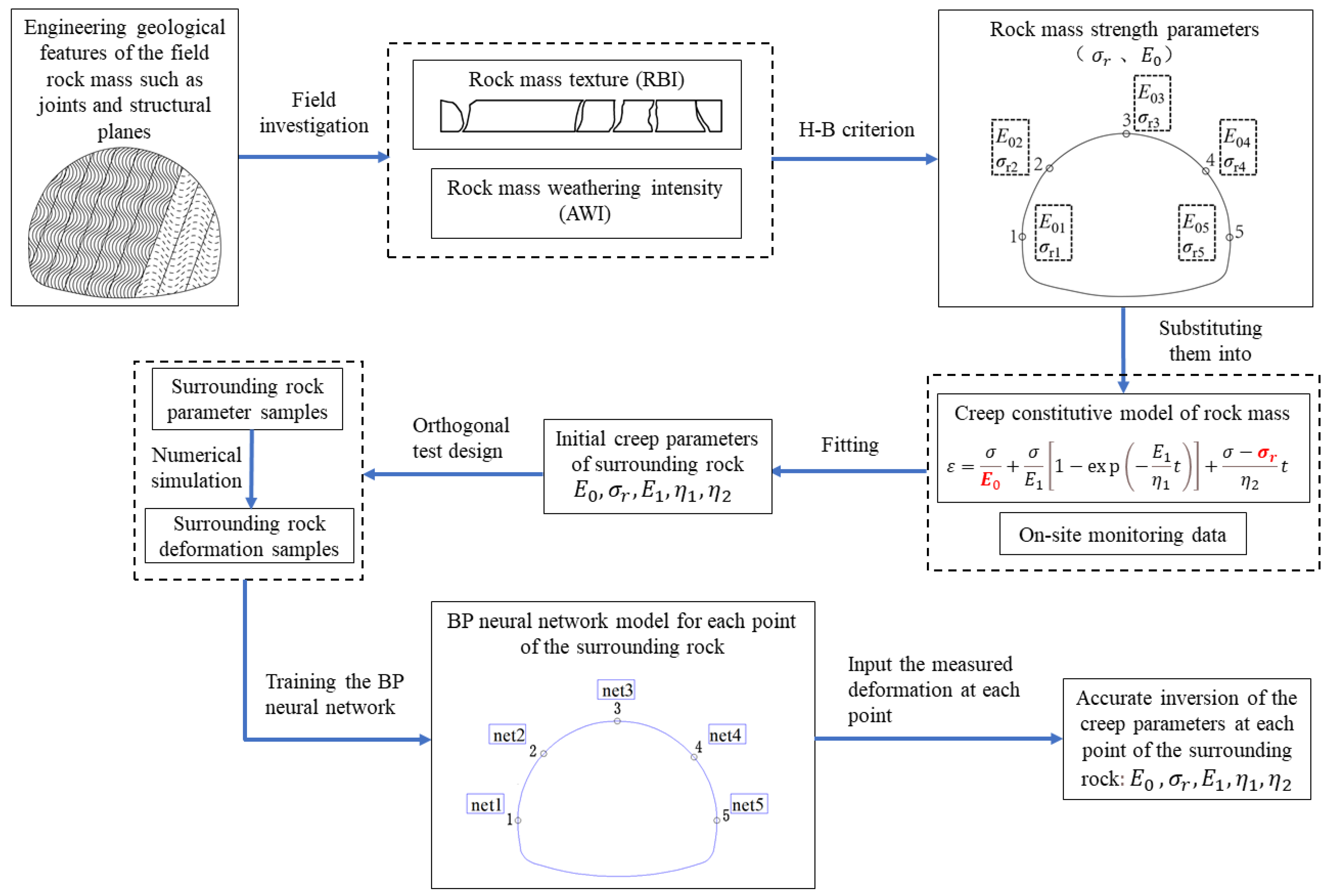
3. Rock Strength and Creep Constitutive Model Based on the Hoek–Brown Failure Criterion
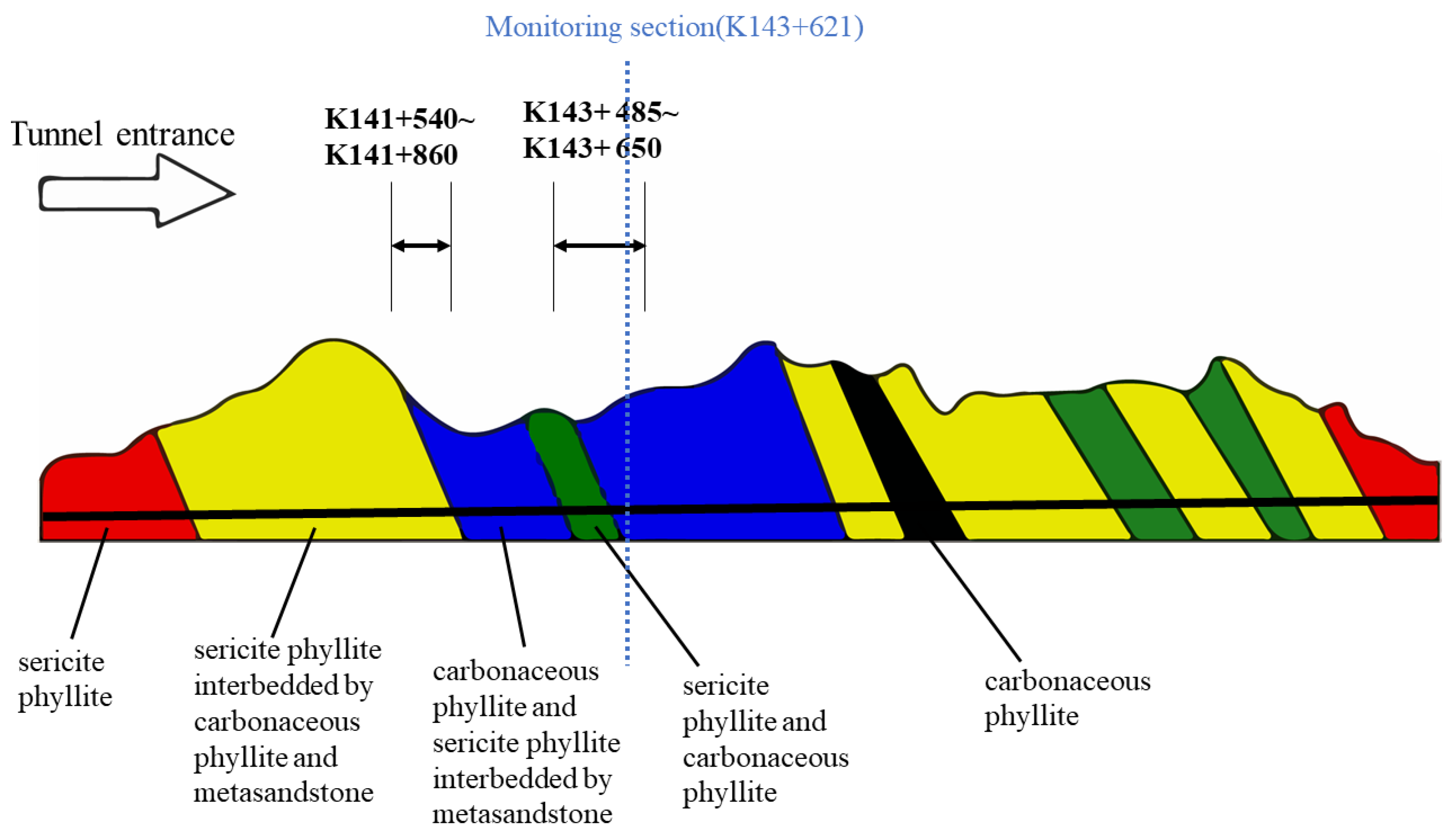
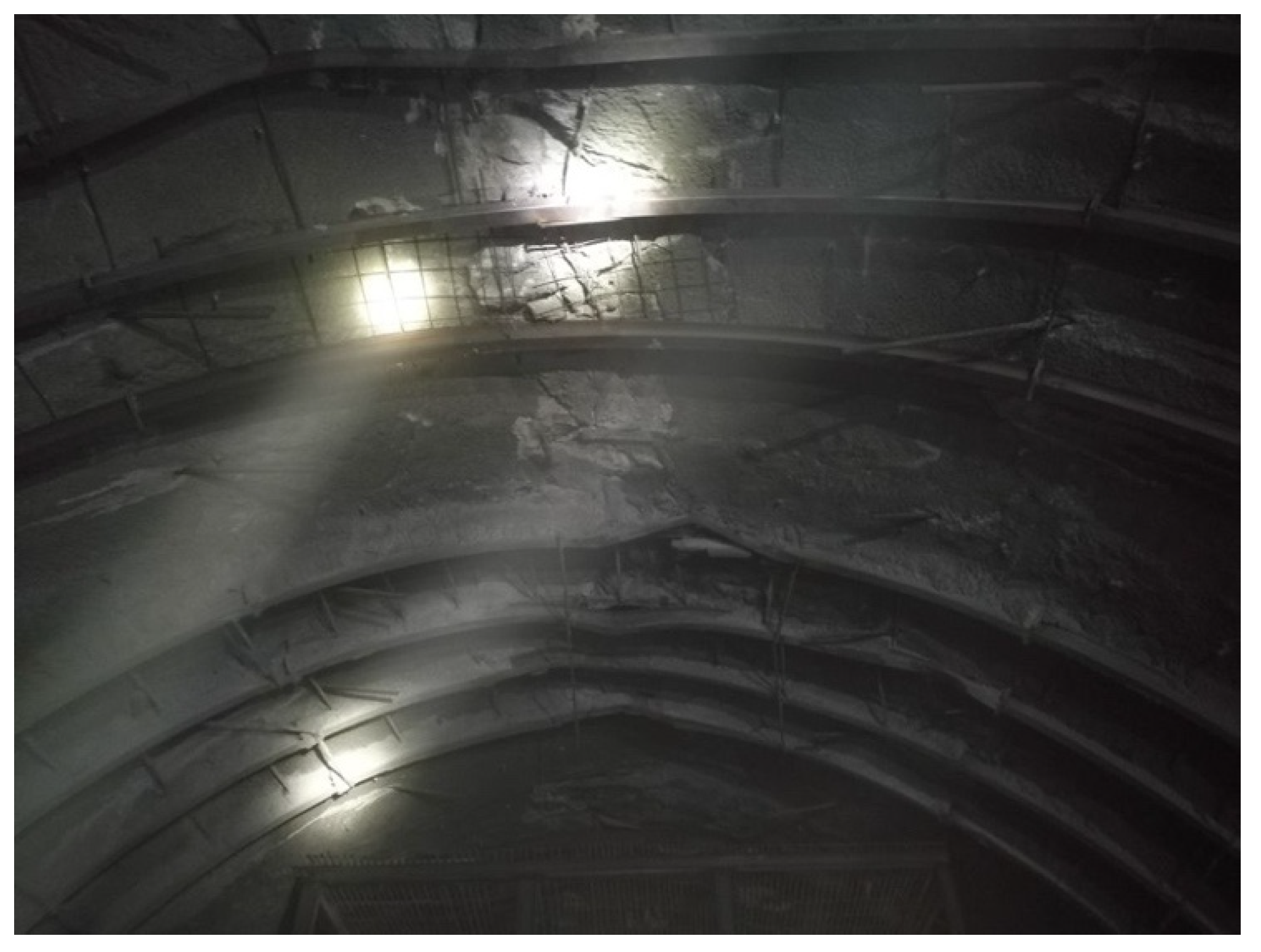
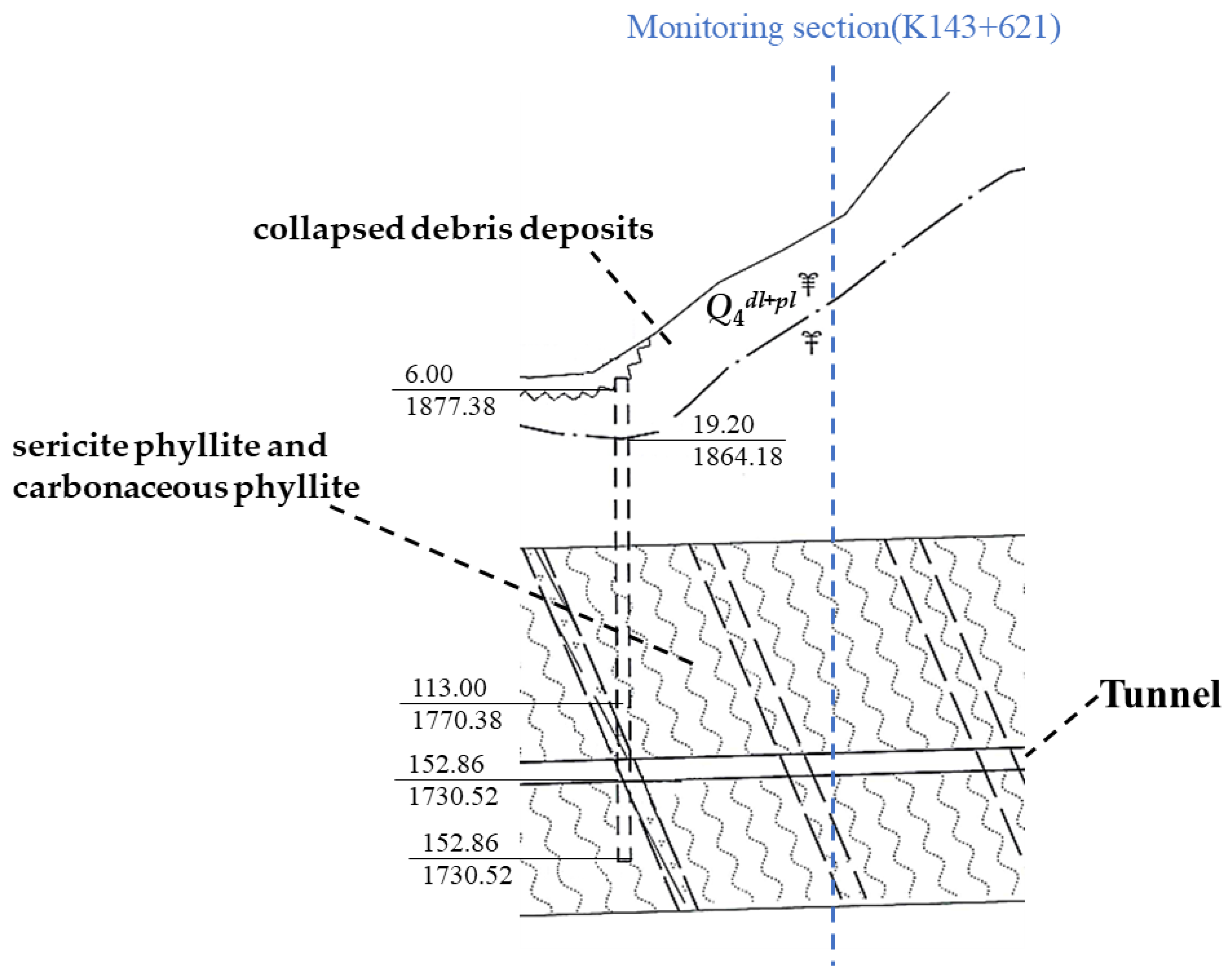
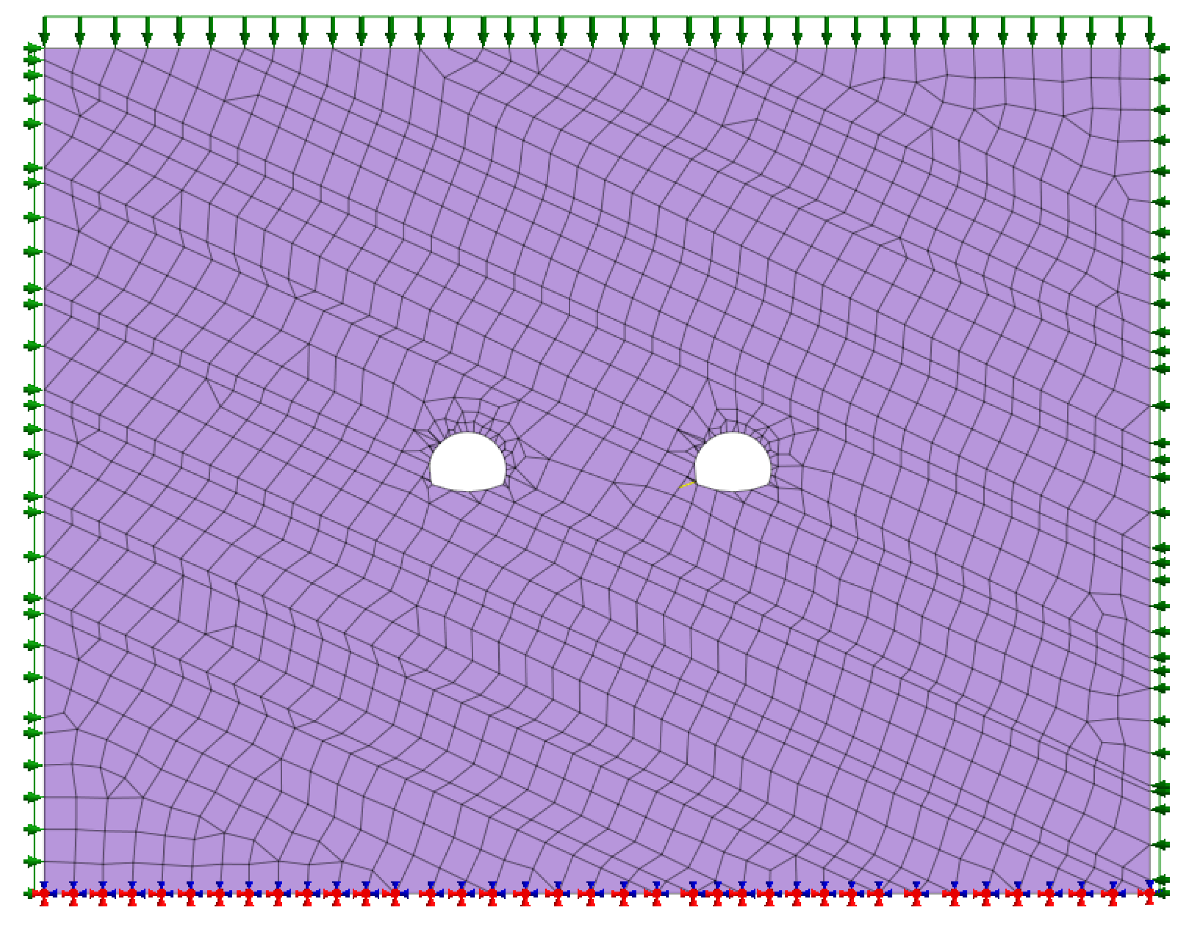
4. Field Application
5. Conclusions
- (1)
- By reviewing the typical cases of large deformation in soft rock tunnels, the main influential factors can be summarized as the lithology combination, weathering effect, and underground water status. With the classical rock mass failure criterion, it is hard to thoroughly incorporate the geological characteristics of the actual rock mass and therefore the semi-empirical semi-theoretical Hoek–Brown approach is more fit-for-purpose.
- (2)
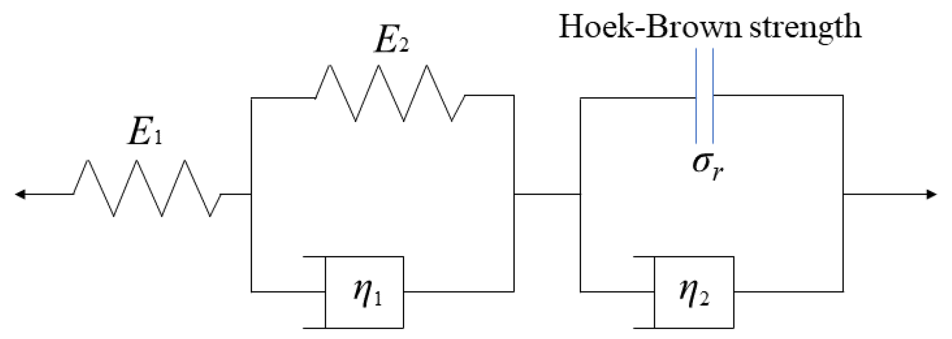
- The geological characteristics of the engineering rock mass were quantitatively characterized using two indexes, namely, the rock mass block index (RBI) and the absolute weathering index (AWI). Following the Hoek–Brown criterion, the long-term strength and elastic modulus of the rock were obtained and then substituted into the rock mass creep constitutive model based on the Nashihara model and the Hoek–Brown failure criterion. By doing so, the original five creep parameters that needed to be determined in the creep equation were reduced to three, which simplifies the calculation of the constitutive model, while well reflecting the engineering, geological, and creep characteristics of the rock mass on site.
- (3)
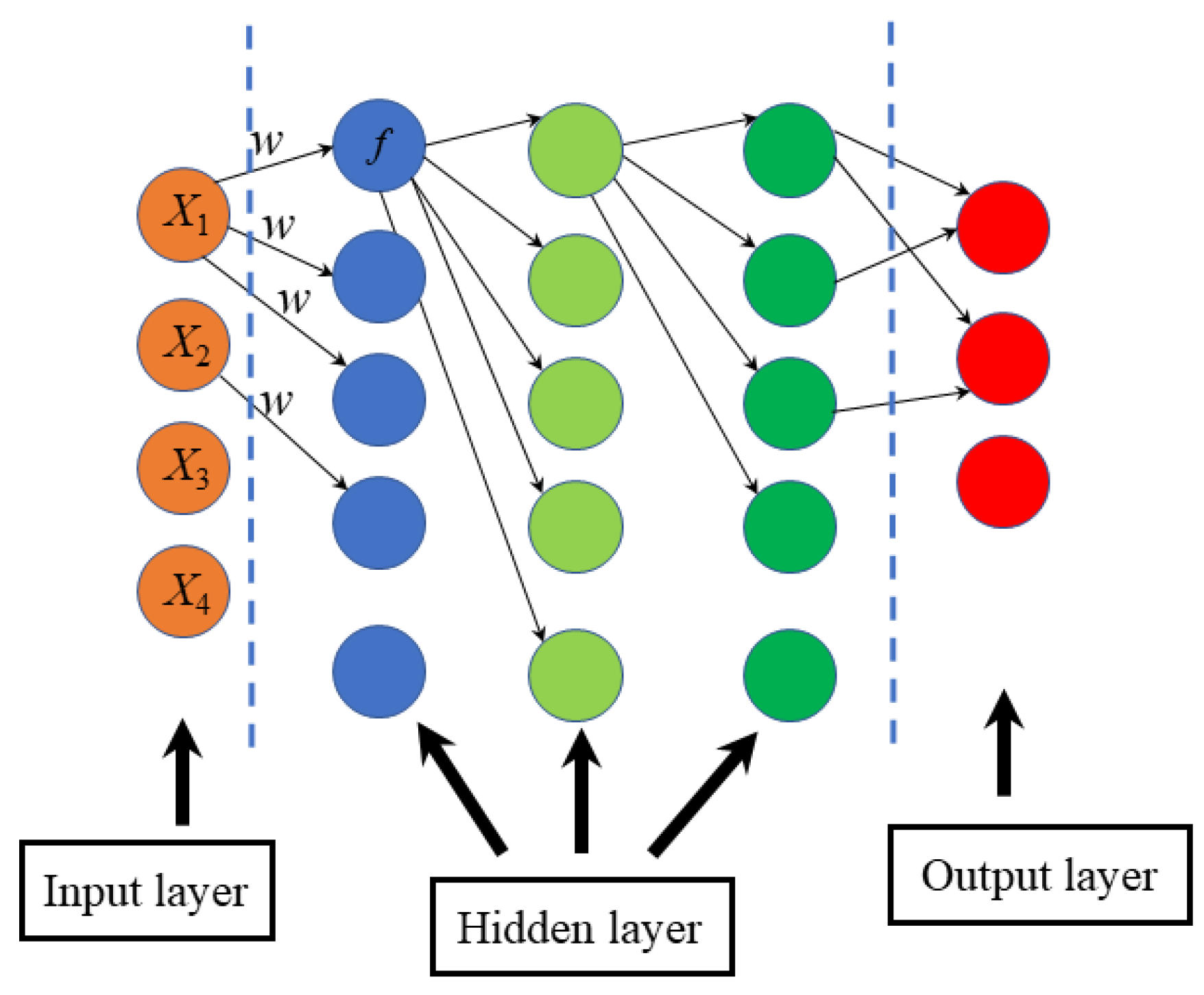
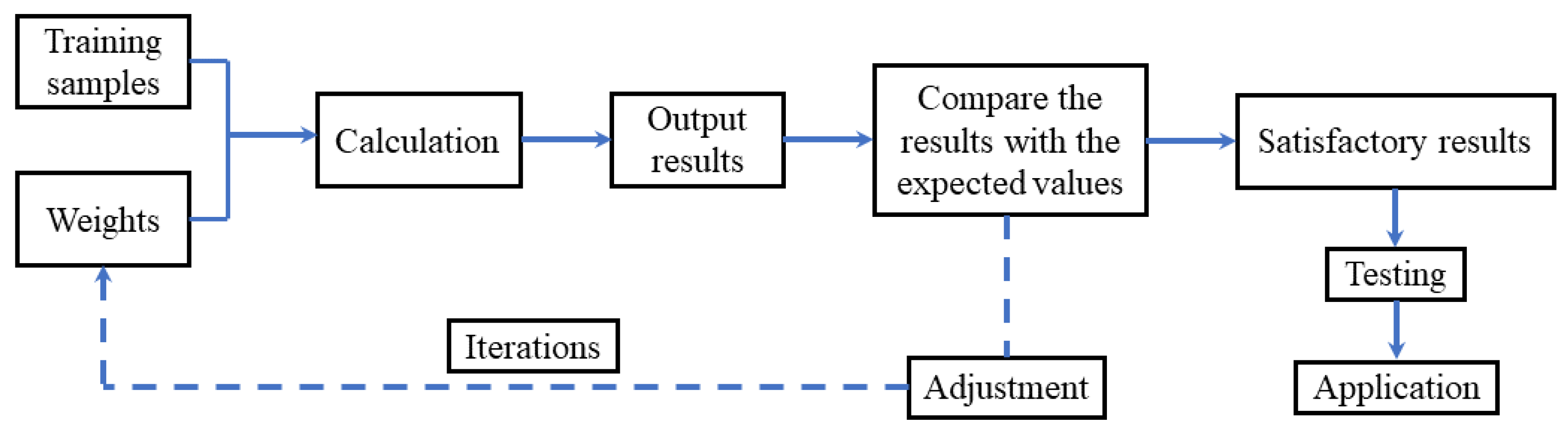
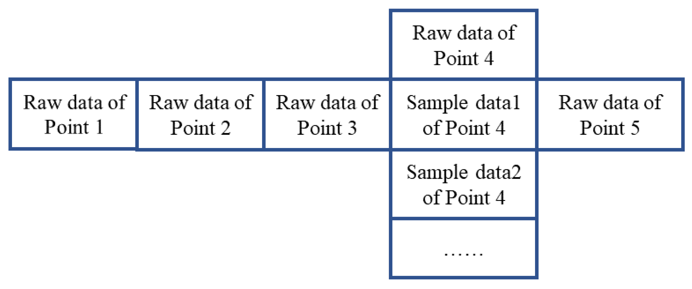
- Considering the fact that the actual engineering geology varies at different positions of the tunnel’s surrounding rock mass, a specific BP neural network model was built for each monitoring point. Then, the rock mass parameters at each point were inverted from the on-site measured deformation. At last, the inverted parameters were input into the numerical model to calculate the deformation at each point, which was compared with the corresponding measured deformation. The resultant errors were all within 15%, satisfying the engineering requirements and demonstrating the reliability of the proposed method.
- (4)
- The values of the rock mass GSI (Figure 2) were all determined according to the engineering geology handbook, relevant standards, and existing literature. Therefore, these values can be adjusted as per the field condition. The inversion of the surrounding rock mass parameters is highly affected by the basic parameters of the engineering geological characteristics and the in-situ stress field of the tunnel’s surrounding rock mass. Hence, during applications of the proposed method, the basic parameters need to be accurately measured to improve the accuracy of the inversion.
- (5)
- This method is suitable for tunneling in unsupported rock mass or plainly supported tunnels after excavation.
Author Contributions
Funding
Institutional Review Board Statement
Informed Consent Statement
Data Availability Statement
Acknowledgments
Conflicts of Interest
References
- He, M.; Jing, H.; Sun, X. Mechanics of Soft Rock Engineering; Science Press: Beijing, China, 2002. [Google Scholar]
- Kong, P.; Jiang, L.S.; Shu, J.M.; Sainoki, A.; Wang, Q.B. Effect of fracture heterogeneity on rock mass stability in a highly heterogeneous underground roadway. Rock Mech. Rock Eng. 2019, 52, 4547–4564. [Google Scholar] [CrossRef]
- Chen, Z.; He, C.; Xu, G.; Ma, G.; Wu, D. A case study on the asymmetric deformation characteristics and mechanical behavior of deep-buried tunnel in phyllite. Rock Mech. Rock Eng. 2019, 52, 4527–4545. [Google Scholar] [CrossRef]
- Jia, P.; Tang, C.; Yang, T.; Wang, S. Numerical Stability Analysis of Surrounding rock mass Mass Layered by Structural Planes with Different Obliquities. J. Northeast Univ. 2006, 27, 1275–1278. [Google Scholar]
- Li, L.; Guan, J.; Xiao, M.; Liu, H.; Tang, K. A creep constitutive model for transversely isotropic rocks. Rock Soil Mech. 2020, 41, 2922–2930, 2942. [Google Scholar]
- Li, C.; Wang, J.; Xie, H. Anisotropic creep characteristics and mechanism of shale under elevated deviatoric stress. J. Pet. Sci. Eng. 2020, 185, 106670. [Google Scholar] [CrossRef]
- Li, A.; Xu, N.; Dai, F.; Gu, G.; Hu, Z.; Liu, Y. Stability analysis and failure mechanism of the steeply inclined bedded rock masses surrounding a large underground opening. Tunn. Undergr. Space Technol. 2018, 77, 45–58. [Google Scholar] [CrossRef]
- Song, D.; Chen, J.; Cai, J. Deformation monitoring of rock slope with weak bedding structural plane subject to tunnel excavation. Arab. J. Geosci. 2018, 11, 251. [Google Scholar] [CrossRef]
- Gao, F.; Guo, J. Stress mechanism and deformation monitoring of bias tunnel. Int. J. Simul. Syst. Sci. Technol. 2016, 17, 14.1–14.4. [Google Scholar] [CrossRef]
- Yin, C.; Li, H.; Che, F.; Li, Y.; Hu, Z.; Liu, D. Susceptibility mapping and zoning of highway landslide disasters in China. PLoS ONE 2020, 15, e0235780. [Google Scholar] [CrossRef]
- Liu, C.H.; Li, Y.Z. Analytical study of the mechanical behavior of fully grouted bolts in bedding rock slopes. Rock Mech. Rock Eng. 2017, 50, 2413–2423. [Google Scholar] [CrossRef]
- Vergara, M.R.; Kudella, P.; Triantafyllidis, T. Large scale tests on jointed and bedded rocks under multi-stage triaxial compression and direct shear. Rock Mech. Rock Eng. 2015, 48, 75–92. [Google Scholar] [CrossRef]
- Li, L.; Tan, Z.S.; Guo, X.L.; Wu, Y.; Luo, N. Large deformation of tunnels in steep dip strata of interbedding phyllite under high geostresses. Chin. J. Rock Mech. Eng. 2017, 36, 1611–1622. [Google Scholar]
- Li, X.H.; Xia, B.W.; Li, D.; Han, C.R. Deformation characteristics analysis of layered rockmass in deep buried tunnel. Rock Soil Mech. 2010, 31, 1163–1167. [Google Scholar]
- Fu, X. Numerical Simulation of Asymmetric Large-Deformation Energy-Releasing Bolt Support for Layered Soft Rock Tunnel; Chengdu Univerisity of Technology: Chengdu, China, 2020. [Google Scholar]
- Li, Z.; Shan, R.; Wang, C.; Yuan, H.; Wei, Y. Study on the distribution law of stress deviator below the floor of a goaf. Geomech. Eng. 2020, 21, 301–313. [Google Scholar] [CrossRef]
- Tian, M.; Han, L.; Meng, Q.; Ma, C.; Zong, Y.; Mao, P. Physical model experiment of surrounding rock mass failure mechanism for the roadway under deviatoric pressure form mining disturbance. KSCE J. Civ. Eng. 2020, 24, 1103–1115. [Google Scholar] [CrossRef]
- Wang, Z.-J.; Luo, Y.-S.; Guo, H.; Tian, H. Effects of initial deviatoric stress ratios on dynamic shear modulus and damping ratio of undisturbed loess in China. Eng. Geol. 2012, 143–144, 43–50. [Google Scholar] [CrossRef]
- Kroon, M.; Faleskog, J. Numerical implementation of a J2 and J3 dependent plasticity model based on a spectral decomposition of the stress deviator. Comput. Mech. 2013, 52, 1059–1070. [Google Scholar] [CrossRef]
- Wang, Q.; Pan, R.; Jiang, B.; Li, S.; He, M.; Sun, H.; Wang, L.; Qin, Q.; Yu, H.; Luan, Y. Study on failure mechanism of roadway with soft rock in deep coal mine and confined concrete support system. Eng. Fail. Anal. 2017, 81, 155–177. [Google Scholar] [CrossRef]
- Wang, W.; Zhang, C.; Wei, S.; Zhang, X.; Guo, S. Whole section anchor–grouting reinforcement technology and its application in underground roadways with loose and fractured surrounding rock mass. Tunn. Undergr. Space Technol. 2016, 51, 133–143. [Google Scholar] [CrossRef]
- Xu, G.; He, C.; Chen, Z.; Yang, Q. Transversely isotropic creep behavior of phyllite and its influence on the long-term safety of the secondary lining of tunnels. Eng. Geol. 2020, 278, 105834. [Google Scholar] [CrossRef]
- Li, X.; Ju, M.; Yao, Q.; Zhou, J.; Chong, Z. Numerical investigation of the effect of the location of critical rock block fracture on crack evolution in a gob-side filling wall. Rock Mech. Rock Eng. 2016, 49, 1041–1058. [Google Scholar] [CrossRef]
- Zhou, J.; Wei, Q.; Liu, G. Back analysis on rock mechanics parameters for highway tunnel by BP neural network method. Chin. J. Rock Mech. Eng. 2004, 23, 941–945. [Google Scholar]
- Cao, W.; Jiang, Y.; Sakaguchi, O.; Li, N.; Han, W. Predication of Displacement of Tunnel Rock Mass Based on the Back-Analysis Method-BP Neural Network. Geotech. Geol. Eng. 2021, 2021, 1–14. [Google Scholar] [CrossRef]
- Wu, Q.; Yan, B.; Zhang, C.; Wang, L.; Ning, G.; Yu, B. Displacement prediction of tunnel surrounding rock mass: A comparison of support vector machine and artificial neural network. Math. Probl. Eng. 2014, 2014, 351496. [Google Scholar] [CrossRef]
- Deng, X.; Xu, T.; Wang, R. Risk evaluation model of highway tunnel portal construction based on BP fuzzy neural network. Comput. Intell. Neurosci. 2018, 2018, 8547313. [Google Scholar] [CrossRef] [Green Version]
- Wen, H.; Yin, J.; Qin, Z.; Xie, R. Application of BP Neural Network to the Back Analysis of Mechanical Parameters of Tunnel Surrounding rock mass. J. Yangtze River Sci. Res. Inst. 2013, 30, 47–51, 56. [Google Scholar]
- He, Y.; Sun, X.; Zhang, Y.; Guo, H.; Li, Q. Intelligent fusion model and analysis method for rock parameter inversion of water diversion tunnel. J. Hydroelectr. Eng. 2021, 40, 114–126. [Google Scholar]
- Ma, F.; Jia, S. Back analysis of elastoplastic parameters of surrounding rock mass for roadway in mudstone and its long-term stability prediction. Rock Soil Mech. 2014, 7, 1987–1994. [Google Scholar]
- Amadei, B. Strength of a regularly jointed rock mass under biaxial and axisymmetric loading conditions. Int. J. Rock Mech. Min. Sci. Geomech. Abstr. 1988, 25, 3–13. [Google Scholar] [CrossRef]
- Xiao, S.; Yang, S. Rock Mass Mechanics; Geological Publishing House: Beijing, China, 1987. [Google Scholar]
- Hoek, E.; Brown, E.T. Practical estimates of rock mass strength. Int. J. Rock Mech. Min. Sci. 1997, 34, 1165–1186. [Google Scholar] [CrossRef]
- Marinos, P.; Hoek, E. Estimating the geotechnical properties of heterogeneous rock masses such as flysch. Bull. Eng. Geol. Environ. 2001, 60, 85–92. [Google Scholar] [CrossRef]
- Hoek, E.; Brown, E.T. The Hoek–Brown failure criterion and GSI–2018 edition. J. Rock Mech. Geotech. Eng. 2019, 11, 445–463. [Google Scholar] [CrossRef]
- Hu, X.; Zhong, P.; Ren, Z. Rock-mass block index and its engineering practice significance. J. Hydraul. Eng. 2002, 33, 80–83. [Google Scholar]
- Parker, A. An index of weathering for silicate rocks. Geol. Mag. 1970, 107, 501–504. [Google Scholar] [CrossRef]
- Su, Y.; Feng, L.; Li, Z.; Zhao, M. Quantification of elements for geological strength index in Hoek-Brown criterion. Chin. J. Rock Mech. Eng. 2009, 28, 36–43. [Google Scholar]
- Li, R.; Wu, L. Research on characteristic indexes of weathering intensity of rocks. Chin. J. Rock Mech. Eng. 2004, 23, 3830. [Google Scholar]


| Tunnel Name | Tunnel Length /m | Buried Depth /m | Lithology | /MPa | Strength of Rock /MPa | Maximum Deformation /mm | Deformation Characteristics | Strain ε = Tunnel Closure/Tunnel Diameter × 100 |
|---|---|---|---|---|---|---|---|---|
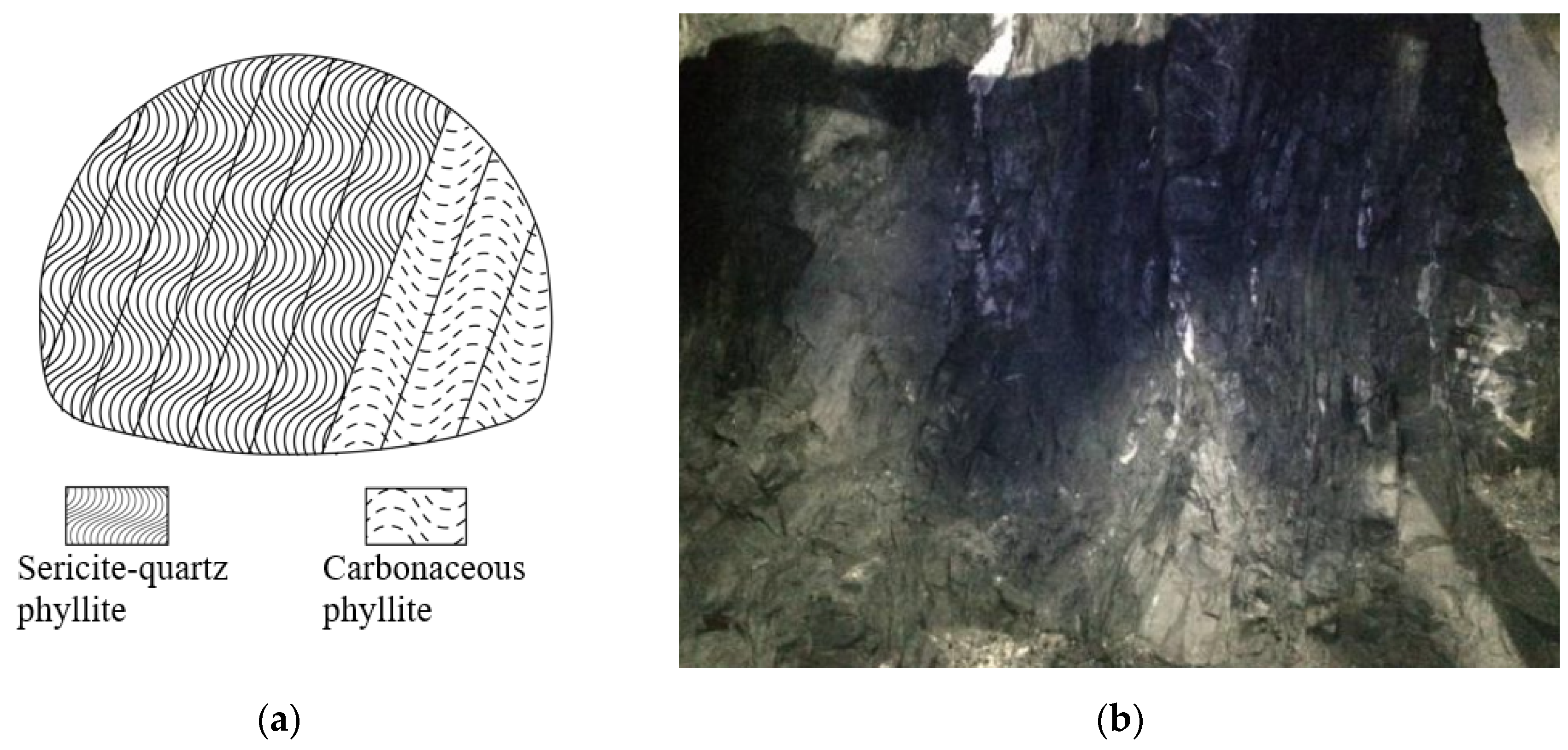
| Maoxian Tunnel, Chenglan Railway | 25,000 | 675 | Sericite phyllite, carbonaceous phyllite | 27.52 | 1.95 | 510 | Compressive large deformation occurs, with prolonged deformation growth and notable time-dependency; horizontal convergence exceeds crown settlement, due to steep inclination of the surrounding rock mass | 8.05 |
| Wuqiaoling Tunne, Lanxin Railway | 20,050 | 1100 | Phyllite, slate | 32.8 | 0.7~2.5 | 1209 | It penetrates the compressive fault; the overall stability of the surrounding rock mass is low; large deformation, early rapid deformation growth, and prolonged duration of deformation are observed due to intensive compression. | 9.69 |
| Zhegushan Tunnel, 317 National Rd. | 4423 | 1000 | Thin layers of carbonaceous phyllite | 17~20 | 12 | 300 | The relatively large magnitude and prolonged duration of surrounding rock mass deformation are manifested as support breakage, steel arch twisting, and their intrusion into tunnel clearance; the tunnel is prone to collapse. | 9.31 |
| Maoyushan Tunnel, Lanyu Railway | 8503 | 700 | Thin bedded slate | 21.28 | 5.63 | 540 | Large rapid deformation, with notable rheological effects; severe twisting and fracturing of the steel arch; horizontal convergence far larger than crown settlement | 8.94 |
| Gonghe Tunnel, Yusha Expressway | 4779 | 1000 | Sandy shale | 29.86 | 11.4 | 200 | Longitudinal cracking and steel frame bending occurs at the initial support of the right spandrel and left arch foot, indicating severe biased compression of the surrounding rock mass | 7.52 |
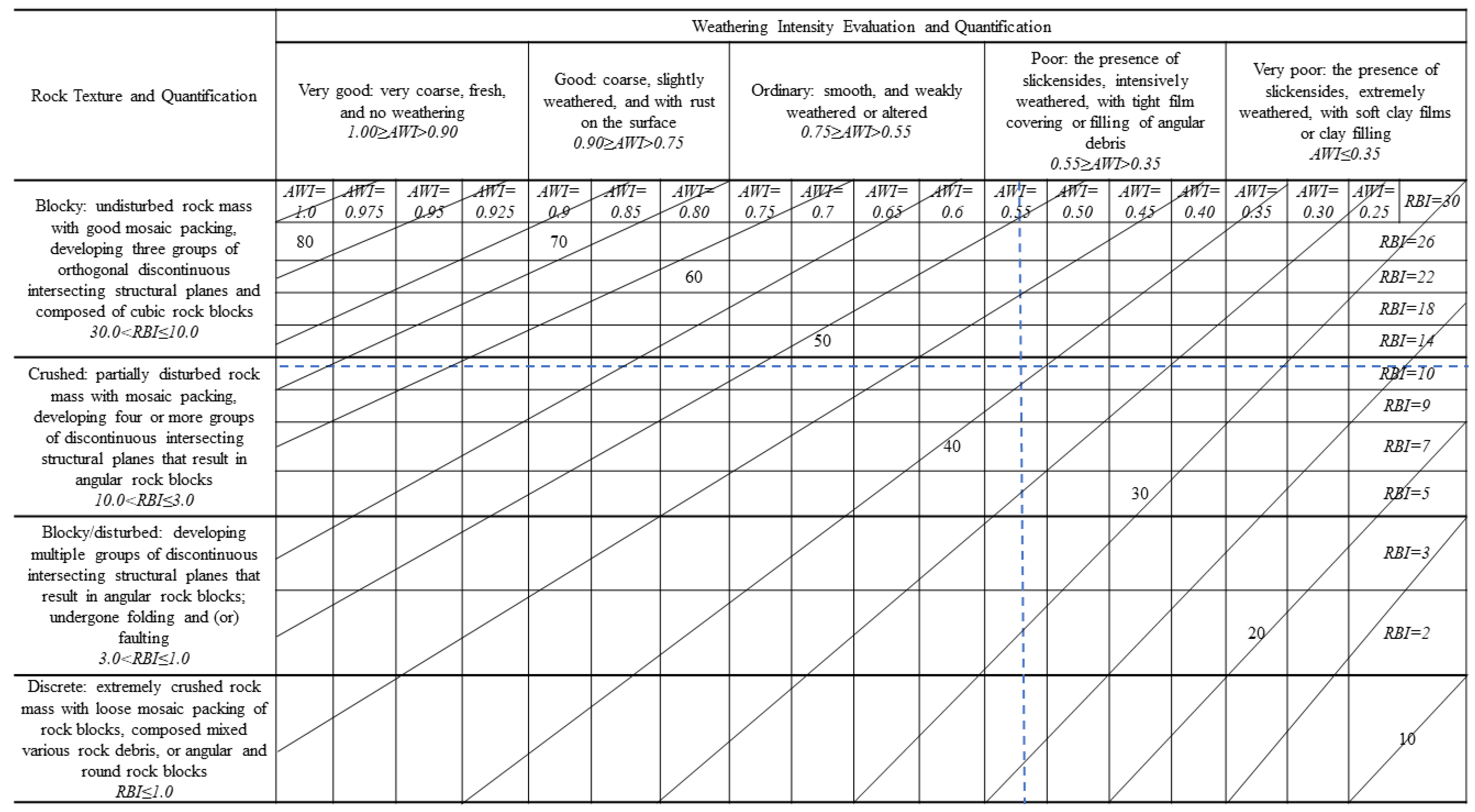
| Texture Type | RBI | Rock Mass Characteristics |
|---|---|---|
| Laminated mosaic texture | 30–10 | Relatively intact, barely, or partially disturbed, often developing 3 groups of structural planes with the spacing of 30–50 cm |
| Mosaic texture | 10–3 | Less intact, mostly disturbed, broken yet with tightly packed fragments, generally developing 3–4 groups of structural planes with the spacing of 10–30 cm |
| Broken texture | 3–1 | Broken rock mass, sufficiently disturbed, composed of fragments or thin layers, with extensive structural planes presenting spacing generally smaller than 10 cm |
| Loose texture | 1–0 | Extremely crushed rock mass, extremely disturbed, composed of loose rock blocks, and angular fragments with crushed debris |
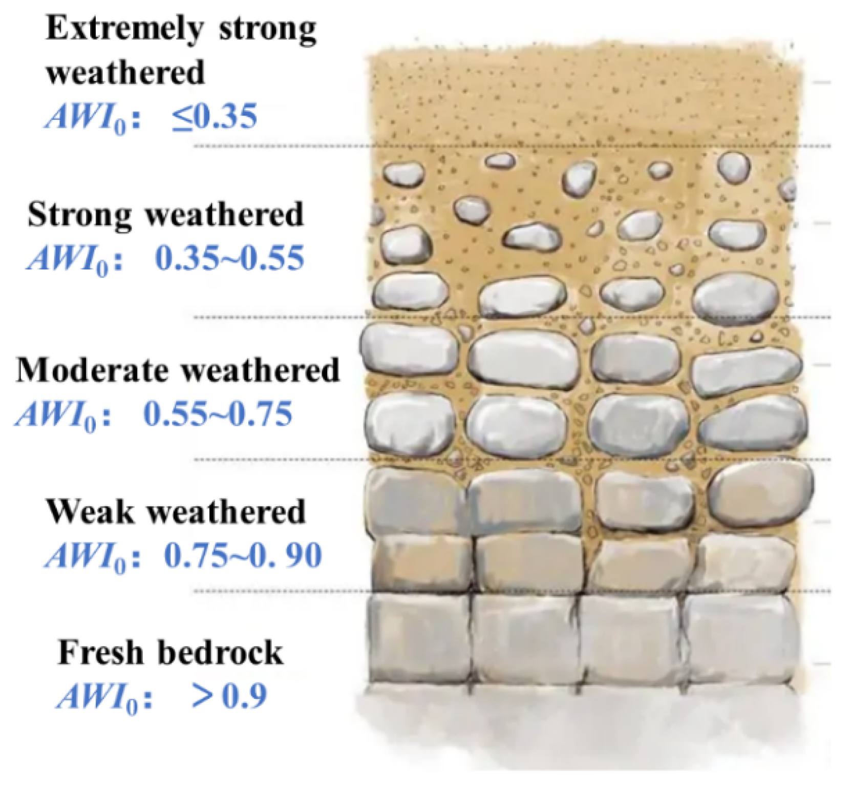
| Weathering Condition | Weathering Characteristics | |
|---|---|---|
| Non-weathered | >0.90 | Very good fracture surface: very coarse, fresh, indicating well-sealed fresh rock matrix and no weathering |
| Slightly weathered | 0.90–0.75 | Good fracture surface: coarse, relatively fresh, with the presence of rush and the slight alteration of minerals with low weathering resistance, indicating slight weathering |
| Weakly weathered | 0.75–0.55 | Ordinary fracture surface: smooth with no filling, partial alteration of minerals with low weathering resistance, indicating weak weathering |
| Intensively weathered | 0.55–0.35 | Poor fracture surface: the presence of slickensides, covering of tight films or filling of angular debris on the surface, high alteration of minerals with low weathering resistance, indicating intensive weathering |
| Extremely weathered | ≤0.35 | Very poor fracture surface: the presence of slickensides, and soft clay films or clay filling; the vast majority of minerals with low weathering resistance are altered; indicating extreme weathering |
| Production Status of Underground Water | RBI Values of Jointed Rock Mass | |||
|---|---|---|---|---|
| 30–10 | 10–3 | 3–1 | 1–0 | |
| Humid or dripping | 0.95 | 0.95–0.89 | 0.89–0.83 | 0.83–0.76 |
| Rain-like or spring-like production with water pressure < 0.1 MPa; or unit water production rate < 10 L/min·m | 0.95–0.89 | 0.89–0.83 | 0.83–0.76 | 0.76–0.71 |
| Rain-like or spring-like production with water pressure > 0.1 MPa; or unit water production rate > 10 L/min·m | 0.89–0.83 | 0.83–0.76 | 0.76–0.71 | 0.71–0.67 |
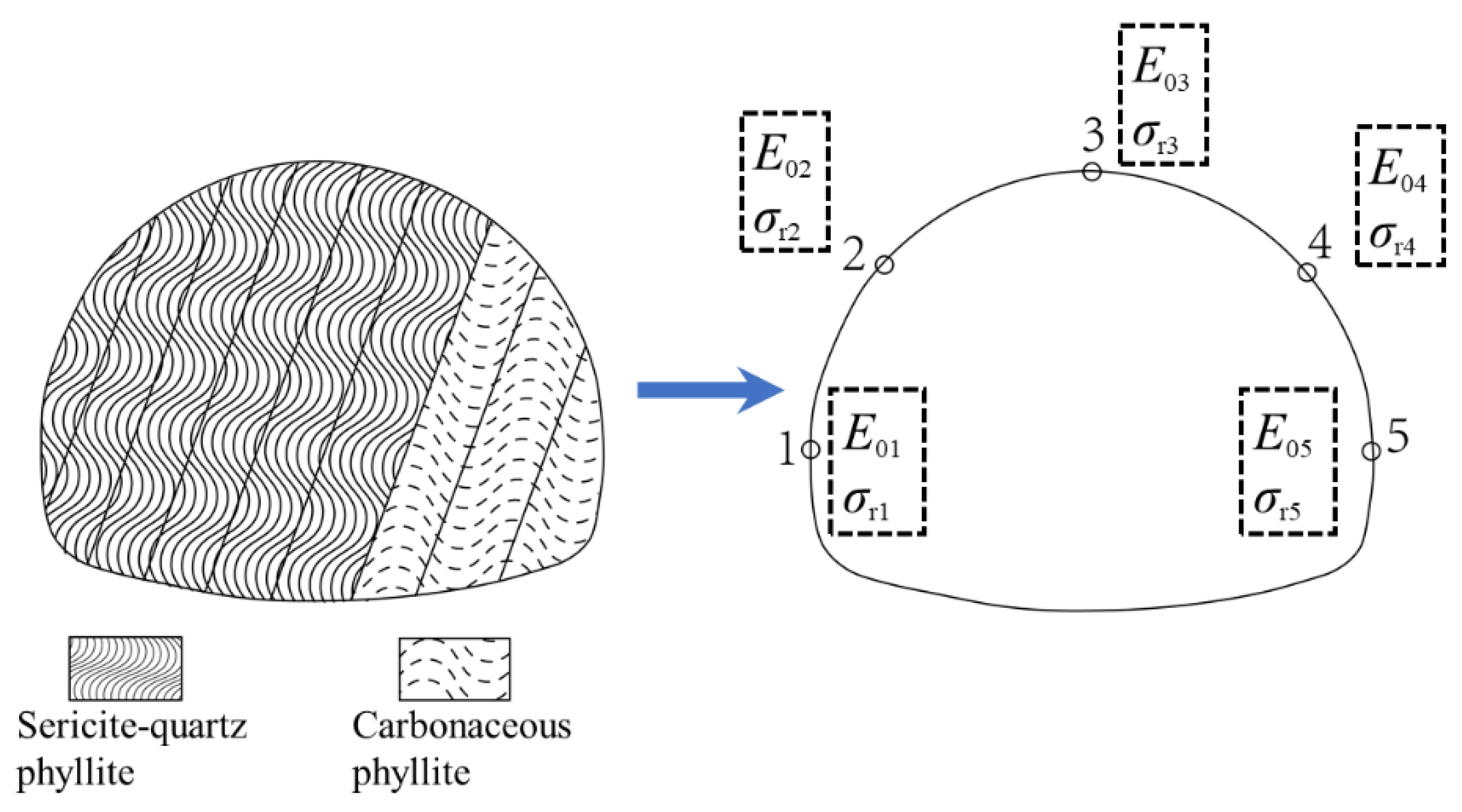
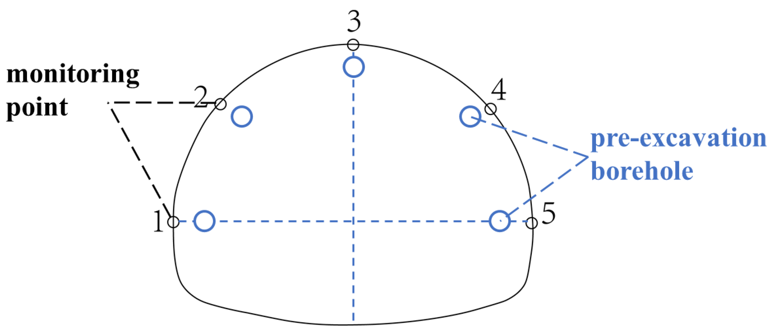
| Monitoring Point | Cores | RBI Values |
|---|---|---|
| 1 |  | 6.763 |
| 2 |  | 5.626 |
| 3 |  | 3.748 |
| 4 |  | 2.8 |
| 5 |  | 4.331 |
| Monitoring Point | RBI | AWI | GSI | s | (MPa) | (MPa) | (GPa) | ||
|---|---|---|---|---|---|---|---|---|---|
| 1 | 6.763 | 1.570 | 79.708 | 2.212 | 0.001418 | 0.27 | 36.8 | 45.29 | 2.69 |
| 2 | 5.626 | 1.306 | 66.305 | 1.840 | 0.001179 | 0.22 | 32.28 | 37.67 | 2.24 |
| 3 | 3.748 | 0.870 | 44.169 | 1.226 | 0.000786 | 0.15 | 21.57 | 25.10 | 1.49 |
| 4 | 2.8 | 0.65 | 33 | 0.916 | 0.000587 | 0.11 | 16.33 | 18.75 | 1.11 |
| 5 | 4.331 | 1.006 | 51.050 | 1.417 | 0.000908 | 0.17 | 22.8 | 29.01 | 1.73 |
| Point No. | |||||
|---|---|---|---|---|---|
| 1 | 2.69 | 36.8 | 0.8 | 16.38 | 93.71 |
| 2 | 2.24 | 32.28 | 0.71 | 11.22 | 88.63 |
| 3 | 1.49 | 21.57 | 0.5 | 8.78 | 6.55 |
| 4 | 1.11 | 16.33 | 0.4 | 7.87 | 5.62 |
| 5 | 1.73 | 22.8 | 0.6 | 10.11 | 78.52 |
| No. | /GPa | /MPa | /GPa | /(GPa·d) | /(GPa·d) | Displacement at Point 1 /mm | Displacement at Point 2 /mm | Displacement at Point 3 /mm | Displacement at Point 4 /mm | Displacement at Point 5 /mm |
|---|---|---|---|---|---|---|---|---|---|---|
| 1 | 2.69 | 36.80 | 0.80 | 16.38 | 93.71 | 7.31 | 9.11 | 13.11 | 27.94 | 11.50 |
| 2 | 2.69 | 41.80 | 1.30 | 21.38 | 98.71 | 12.51 | 15.59 | 22.43 | 47.80 | 19.67 |
| 3 | 2.69 | 46.80 | 1.80 | 26.38 | 103.71 | 11.02 | 13.74 | 19.76 | 42.11 | 17.33 |
| 4 | 2.69 | 51.80 | 2.30 | 31.38 | 108.71 | 9.84 | 12.27 | 17.64 | 37.60 | 15.47 |
| 5 | 2.69 | 56.80 | 2.80 | 37.38 | 113.71 | 8.90 | 11.09 | 15.95 | 34.00 | 13.99 |
| 6 | 2.24 | 36.80 | 1.30 | 26.38 | 108.71 | 15.83 | 19.73 | 25.85 | 33.66 | 22.41 |
| 7 | 2.24 | 41.80 | 1.80 | 31.38 | 113.71 | 14.31 | 17.84 | 23.37 | 30.43 | 20.26 |
| 8 | 2.24 | 46.80 | 2.30 | 37.38 | 93.71 | 11.76 | 14.66 | 19.21 | 25.01 | 16.65 |
| 9 | 2.24 | 51.80 | 2.80 | 16.38 | 98.71 | 17.73 | 22.10 | 28.95 | 37.70 | 25.10 |
| 10 | 2.24 | 56.80 | 0.80 | 21.38 | 103.71 | 10.91 | 13.60 | 17.82 | 23.20 | 15.45 |
| 11 | 1.49 | 36.80 | 1.80 | 37.38 | 98.71 | 10.60 | 13.21 | 18.74 | 30.89 | 16.44 |
| 12 | 1.49 | 41.80 | 2.30 | 16.38 | 103.71 | 8.71 | 10.85 | 15.40 | 25.38 | 13.51 |
| 13 | 1.49 | 46.80 | 2.80 | 21.38 | 108.71 | 14.90 | 18.57 | 26.35 | 43.43 | 23.11 |
| 14 | 1.49 | 51.80 | 0.80 | 26.38 | 113.71 | 13.13 | 16.36 | 23.22 | 38.26 | 20.36 |
| 15 | 1.49 | 56.80 | 1.30 | 31.38 | 93.71 | 11.72 | 14.61 | 20.73 | 34.16 | 18.18 |
| 16 | 1.11 | 36.80 | 2.30 | 21.38 | 113.71 | 23.73 | 28.05 | 40.76 | 51.49 | 34.56 |
| 17 | 1.11 | 41.80 | 2.80 | 26.38 | 93.71 | 20.91 | 24.71 | 35.91 | 45.37 | 30.45 |
| 18 | 1.11 | 46.80 | 0.80 | 31.38 | 98.71 | 18.67 | 22.07 | 32.06 | 40.51 | 27.19 |
| 19 | 1.11 | 51.80 | 1.30 | 37.38 | 103.71 | 16.88 | 19.95 | 28.99 | 36.62 | 24.58 |
| 20 | 1.11 | 56.80 | 1.80 | 16.38 | 108.71 | 13.87 | 16.39 | 23.82 | 30.09 | 20.20 |
| 21 | 1.73 | 36.80 | 2.80 | 31.38 | 103.71 | 18.26 | 21.85 | 25.08 | 31.69 | 21.27 |
| 22 | 1.73 | 41.80 | 0.80 | 37.38 | 108.71 | 16.31 | 19.51 | 18.12 | 22.89 | 15.37 |
| 23 | 1.73 | 46.80 | 1.30 | 16.38 | 113.71 | 14.74 | 17.64 | 16.39 | 20.70 | 13.89 |
| 24 | 1.73 | 51.80 | 1.80 | 21.38 | 93.71 | 12.12 | 14.49 | 13.46 | 17.01 | 11.42 |
| 25 | 1.73 | 56.80 | 2.30 | 26.38 | 98.71 | 20.73 | 24.80 | 33.23 | 41.46 | 28.48 |
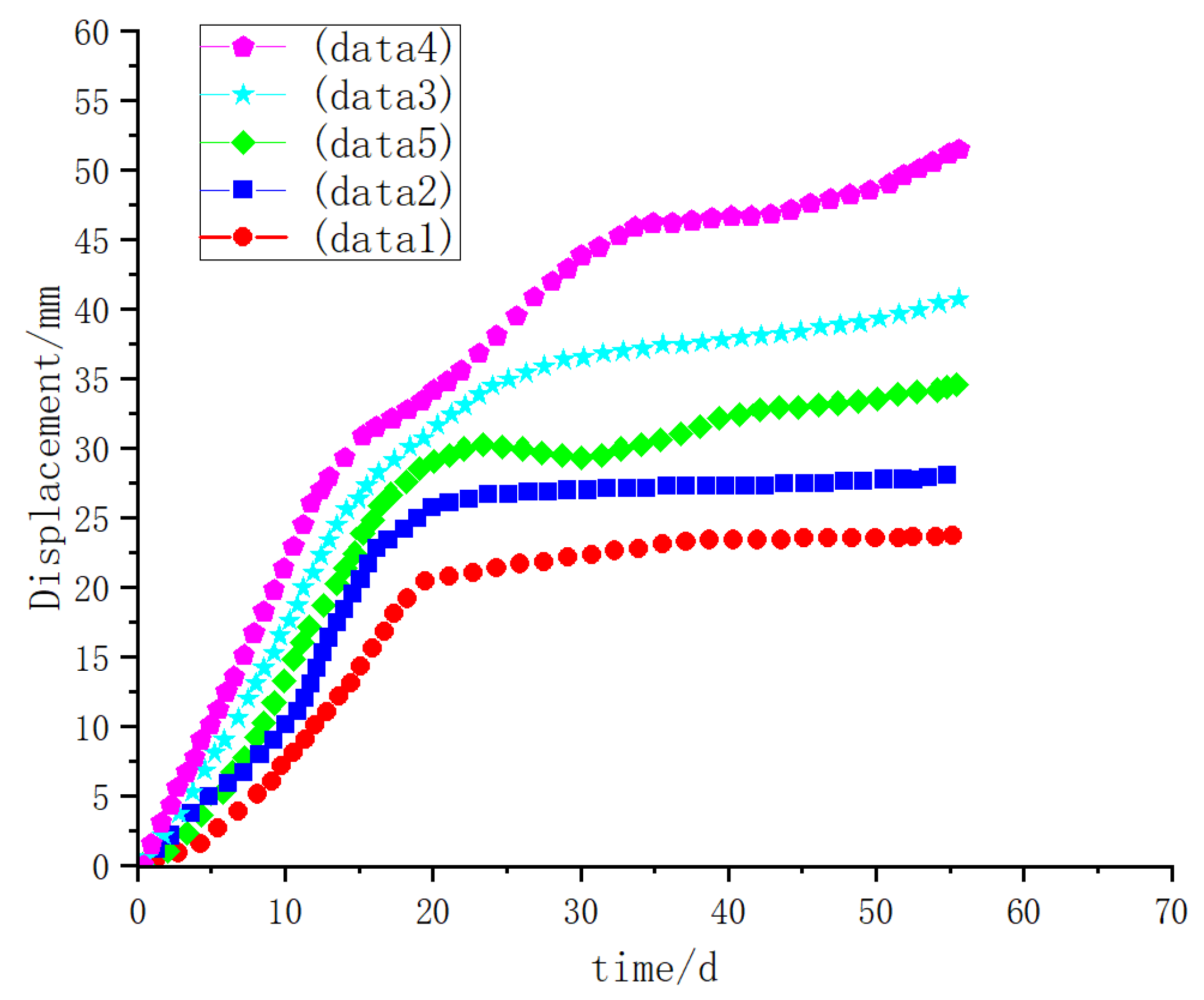
| Monitoring Point | Measured Deformation /mm | Output: Inverted Mechanical Parameters of the Surrounding Rock Mass | Simulated Deformation /mm | Relative Error /% | ||||
|---|---|---|---|---|---|---|---|---|
/GPa | /MPa | /GPa | /(GPa·d) | /(GPa·d) | ||||
| 1 | 23.73 | 3.44 | 35.35 | 0.92 | 16.85 | 104.49 | 26.67 | 12.37 |
| 2 | 28.05 | 2.91 | 31.89 | 0.81 | 12.39 | 97.20 | 30.69 | 9.41 |
| 3 | 40.76 | 2.12 | 21.67 | 0.59 | 10.01 | 9.13 | 45.57 | 11.81 |
| 4 | 51.50 | 1.71 | 16.91 | 0.48 | 9.19 | 8.11 | 58.54 | 13.67 |
| 5 | 34.56 | 2.39 | 22.63 | 0.71 | 11.15 | 88.00 | 37.51 | 8.53 |
Publisher’s Note: MDPI stays neutral with regard to jurisdictional claims in published maps and institutional affiliations. |
© 2021 by the authors. Licensee MDPI, Basel, Switzerland. This article is an open access article distributed under the terms and conditions of the Creative Commons Attribution (CC BY) license (https://creativecommons.org/licenses/by/4.0/).
Share and Cite
Chen, C.; Li, T.; Ma, C.; Zhang, H.; Tang, J.; Zhang, Y. Hoek-Brown Failure Criterion-Based Creep Constitutive Model and BP Neural Network Parameter Inversion for Soft Surrounding Rock Mass of Tunnels. Appl. Sci. 2021, 11, 10033. https://doi.org/10.3390/app112110033
Chen C, Li T, Ma C, Zhang H, Tang J, Zhang Y. Hoek-Brown Failure Criterion-Based Creep Constitutive Model and BP Neural Network Parameter Inversion for Soft Surrounding Rock Mass of Tunnels. Applied Sciences. 2021; 11(21):10033. https://doi.org/10.3390/app112110033
Chicago/Turabian StyleChen, Chao, Tianbin Li, Chunchi Ma, Hang Zhang, Jieling Tang, and Yin Zhang. 2021. "Hoek-Brown Failure Criterion-Based Creep Constitutive Model and BP Neural Network Parameter Inversion for Soft Surrounding Rock Mass of Tunnels" Applied Sciences 11, no. 21: 10033. https://doi.org/10.3390/app112110033