Article

Simulation and Optimization for a Closed-Loop Vessel Dispatching Problem in the Middle East Considering Various Uncertainties

1
Research Center of Digital Supply Chain and Operations, Department of Engineering Systems Management, Khalifa University, Abu Dhabi 127788, United Arab Emirates
2
Advanced Materials Research Center, Technology Innovation Institute, Abu Dhabi 127788, United Arab Emirates
*
Author to whom correspondence should be addressed.
Appl. Sci. 2021, 11(20), 9626; https://doi.org/10.3390/app11209626
Submission received: 29 July 2021 / Revised: 27 September 2021 / Accepted: 12 October 2021 / Published: 15 October 2021
(This article belongs to the Special Issue Smart Service Technology for Industrial Applications)

Abstract

:
The downstream sectors of the hydrocarbon industry in the Middle East are growing quickly. Due to their geographical locations, they need to transport products from manufacturing plants at one port to other hub ports for international shipping, forming complex closed-loop shipping systems. Such domestic shipping systems are also typical logistics structures in many energy and heavy industries near coastal regions. The operations in such systems are frequently lagging due to uncertainties, such as weather and unexpected events, and the lack of effective management techniques. More reliable and efficient systems require a better vessel operations management policy than one based on a first-available-first-use policy and constant voyage speed. This study develops a detailed and realistic simulation model to evaluate the economic and environmental performance of a closed-loop vessel shipping system, considering various uncertainties from weather and port operations. Furthermore, the optimization model has been incorporated into the simulation model to prescribe the optimal number of vessels and voyage speed to minimize the total costs. A new vessel dispatching policy, large-vessel-first-use, has been proposed and compared with the first-available-first-use policy using the developed model. Increased use of large vessels and slower voyage speeds significantly benefited the total costs and environmental effects. The optimal solution presented the potential to save 26.8% of the total cost and reduce greenhouse gas emissions up to 39% compared with the current operating condition.

1. Introduction

The Middle East is well established as a crude oil and natural gas exporter and now is expanding investment in the refining and petrochemicals market. The International Energy Agency has reported that refinery output from the Middle East is set to increase by 60% by 2040 [1]. Therefore, it is anticipated that reliance on the supply chain’s ability to facilitate the transportation of petrochemical products will significantly increase. The particle-type petrochemical products, such as polyethylene and polypropylene, are usually packaged in a container and transported by a container ship, allowing transshipment at a port.
The geographical features of the Middle East usually force manufacturers to transport hydrocarbon products from manufacturing sites near one port to a few hub ports for international shipping. Such domestic shipping systems generally form a closed-loop shipping system with dedicated vessels and require infrastructure management. Manufacturers need integrated management to handle vessel operations and related infrastructure, entailing various issues and complexity.
In particular, bad weather is one of the most difficult challenges in maritime transportation because it randomly hinders vessels from traveling at sea. At high wind speeds above a critical level, vessels cannot start to travel or may need to decrease speed if they were already at sea [2]. In addition, low visibility increases the risk of collision between vessels and obstacles. Some common causes of reduced visibility include fog, mist, smoke, heavy rains, and bright flashes from reflected sunlight [3]. A visibility distance of less than one nautical mile is hazardous as it reduces a vessel’s ability to sail safely, and a visibility distance of less than half a mile implies that vessels should not leave port [4].
Moreover, green shipping management has become a vital topic in the shipping industry. The shipping industry is responsible for a significant environmental footprint as it accounts for 2.7% of global CO2 emissions [5]. The International Maritime Organization (IMO) issued the Global Sulfur Cap 2020 regulation to limit sulfur oxide emissions for ships to below 0.5% compared to the previous limit of 3.5% [6]. The IMO also aims to reduce greenhouse gas (GHG) emissions by at least 50% by 2050 compared to 2008 [7]. Regulatory changes related to GHG emissions and waste discharge have generated more pressure for the shipping industry, requiring better environmental performance [8].
Many studies used simulation tools to address various issues and facilitate and improve related cargo shipping systems in the oil and gas industry and other industries. Cheng and Duran (2004) addressed a global crude oil transportation model using simulation [9]. They also formulated a design and control problem as a Markov decision process incorporating uncertainties such as travel time and crude demand. Using Bayesian simulation techniques, Merrick et al. (2005) [10] studied the impact of ferry service expansions, considering uncertainties such as the arrival times of vessels. Franzese et al. (2006) [11] combined a template modeling with simulator-style development to yield a customized template for petrochemical supply chain operations, characterizing the downstream supply chain elements, including refineries and transportation modes. Almaz and Altiok (2012) [12] analyzed the risk of three different alternatives for improvement, such as increasing vessel arrival, deepening the river, and using larger vessels.
Further, Kulak et al. (2013) [13] analyzed terminal operations and detected system bottlenecks to highlight possible improvements. A simulation-based optimization approach by Ilati et al. (2014) [14] identified that tugboat deficiency contributed to increased waiting times for vessels, and low tugboat utilization had economic consequences. Carotenuto et al. (2014) [15] adopted a simulation-based approach to evaluate the primary supply process of maritime transport carrying crude oil. They highlighted that reducing inventory variance impacted the system operations positively and provided economic benefits by reducing costs. Recently, Rahimikelarijani et al. (2018) [16] used a simulation approach for congestion avoidance in waterways to operate with shorter waiting times and higher throughput by applying the Fisher pairwise comparison method.
Mathematical programming is another primary approach used to address vessel shipping operations. Lababidi et al. (2004) [17] addressed uncertainties in operations and economic costs in the petrochemical sector using a two-stage stochastic optimization approach. Saharidis et al. (2009) [18] formulated a mixed-integer linear programming (MILP) model to determine the unloading and loading times of crude oil at a port and developed a few valid inequalities to solve the problem effectively. The two-stage stochastic model in [19] addressed the optimization of investment planning for the distribution of petroleum products under uncertainty, providing a specific case study in northern Brazil.
Further, the optimization model in [20] addressed ship routing and scheduling problems in crude oil transportation with split deliveries. He et al. (2014) [21] formulated an MILP model for multi-echelon container supply-chain networks to minimize the total supply-chain service costs. Ghezavati et al. (2015) [22] designed a downstream segment for a supply chain system in the petroleum industry. Their developed optimization model coupled with a simulation model prescribed the optimal locations of facilities and their capacities.
Ye et al. (2017) [23] formulated two MILP models for a scheduling problem to transport refined oil products using tramp ships. Aydin et al. (2017) [24] adopted a dynamic programming approach to address the speed optimization problem in liner shipping. Recently, An et al. (2019, a) [25] presented a MILP model for integrated scheduling of vessel dispatching and port operations for the closed-loop shipping system in the context of deterministic parameters with a constant travel speed.
Few studies addressed the closed-loop container shipping system with uncertainty. To the best of our knowledge, only Bahamaish et al. (2019) [26] handled the closed-loop container shipping system with uncertainty using simulation. They considered the uncertain round-trip time incurred by uncontrollable, unexpected events at destination ports. Using a fixed number of vessels, they examined the opportunity for cost savings by adjusting vessel operation policies.
The number of vessels and their voyage speed are vital factors and may have a trade-off for system performance. Considering additional existing uncertainties such as bad weather may generate more reliable and realistic estimates. Therefore, this study extends to the work of Bahamaish et al. (2019) by incorporating new decision factors for the numbers of each type of vessel and forward and backward travel speeds into the simulation model. We also consider additional uncertainties from high wind and low visibility to model the uncertain voyage interruption in the system.
Hence, the first objective of this study is to develop a detailed and realistic simulation model for the closed-loop vessel dispatching problem to transport petrochemicals with several uncertainties caused by bad weather and uncontrollable events at destination ports. The second objective is to devise the best vessel operational policies to reduce operating costs in an environmentally friendly manner, considering the different number of vessels and various travel speeds.
The remainder of this paper is organized as follows: Section 2 demonstrates the problem statement and an approach to solving the current issues. Section 3 describes the developed simulation and optimization models and presents the newly devised vessel operating policies. Section 4 provides the cases and data for numerical studies, and Section 5 analyzes and discusses the results. Finally, Section 6 presents the conclusions.

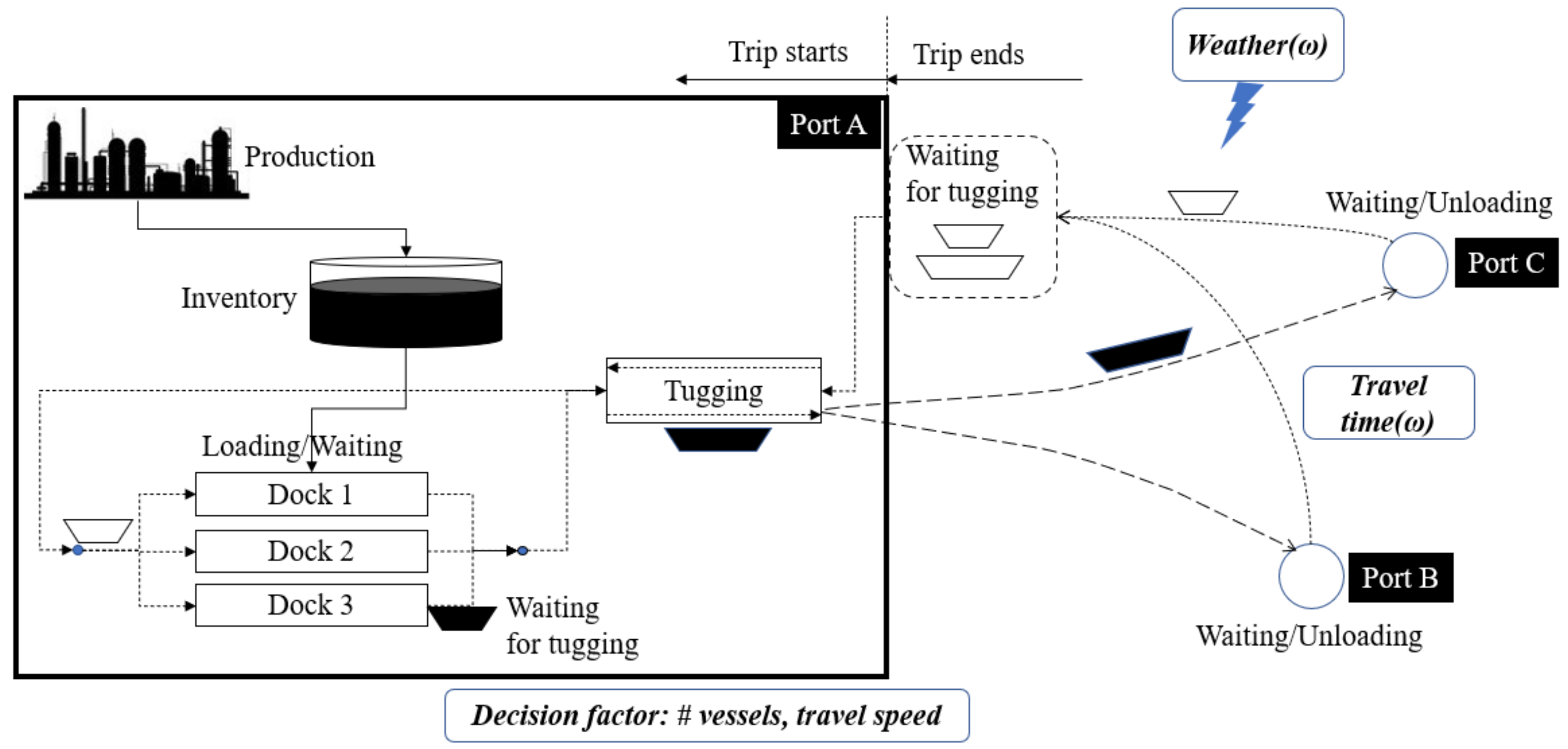
2. Problem Statement

In the proposed scenario, the geographical location of a petrochemical plant in the UAE requires transporting products from a manufacturing plant near one port to two other ports for international shipping. The fundamental system structure is based on the system studied in [26]. Figure 1 depicts the schematic structure of the considered system. For domestic shipping, different types of vessels (i.e., small and large) transport products from the port at the manufacturing plant to other international ports and return to the origin port for another shipment. Such a back-and-forth voyage continues, forming a closed-loop system. This study incorporates uncertainties from bad weather and round-trip time into the system. It also considers new decision factors, such as the number of each type of vessel and forward and backward travel speeds.
We have employed a few assumptions to construct the problem. First, we assume that the products are packed in a container and are ready to be loaded onto a ship. Second, the vessels berthed at the origin port are assumed to wait until they are fully loaded. Third, according to the field experts’ comments, vessels on the voyage are assumed to continue to travel to the destination port, regardless of weather conditions. Lastly, we assume that only one aggregated type of product is transported.
A vessel’s trip begins from the waiting area in near-coastal water from the origin port, Port A. Because Port A has three docks, up to three vessels of any size can be berthed simultaneously and load products packaged in a container. The vessels in the waiting area stay there until any dock becomes available. A specific sea area adjacent to Port A is dedicated for use by arriving and departing tugging. For safety in the coastal waters of the origin port, both arriving and departing tugging is performed one by one in each 3 h time slot like a single runway at an airport.
Once a vessel departs, it travels to Port B or Port C. Because the destination ports are managed by other organizations and used by many other companies, the manufacturing company has no control over the operations at the other ports. In contrast, it can control and manage all the operations at Port A and related infrastructure. Thus, unloading at Ports B and C is often delayed due to the uncertainties of terminal availability. Accordingly, a round-trip time, which includes times for the forward and backward voyages and unloading at the destination port, is somewhat uncertain. After unloading the products and loading empty containers, the vessel returns to Port A. Then, one cycle of a vessel trip is completed. Because the manufactured products always need to be transported to the international ports (i.e., Ports B and C), the travel cycle is repeated as often as needed.
The controllable operations at the origin port (e.g., tugging, loading and unloading, and waiting) follow the operation schedules determined by a manager and the inter-returning pattern of vessels. Therefore, the uncertain returning pattern may impose difficulties on scheduling vessel operations at the origin port. In particular, the voyage could be interrupted by uncertain weather conditions. In the considered system, vessels cannot depart from ports when a wind speed exceeds 35 km/h or a visibility distance is less than 1 km. This study also considers such an uncertain voyage interruption along with the uncertain delay at the destination ports.
Currently, the manufacturing company rents several vessels for a specific period (three years) and operates vessels at the origin port based on the first-available-first-use (FAFU) policy. The vessels usually travel at 22.2 km/h (12 knots). Thus, it would be worth examining the impact of differentiating the numbers of each type of vessel and forward and backward travel speeds on the system performance compared with the current operating conditions. Eventually, the optimal operating conditions should be prescribed to minimize the total costs considering the environmental effect.
Note that the components and structure of the considered system are very similar to the round-trip aviation transportation system, which includes boarding and operations at the departing airport terminals, flying, landing and disembarking to the destination airport, and returning [27]. Such structural similarity implies that the closed-loop shipping system management is not trivial and may involve as many complicated and challenging managerial factors as the aviation transportation system. Another type of closed-loop transportation system can be found in biomass collection using trucks [28].

3. Methods

This section describes the methods used in this study for simulation modeling, the optimization model embedded in simulation, and the environmental analysis.

3.1. Simulation Modeling

This study uses Simio simulation software to build a simulation model. The following subsections provide detailed descriptions of the developed simulation model, validation procedure, output, and new scheduling policies tested by the developed model.

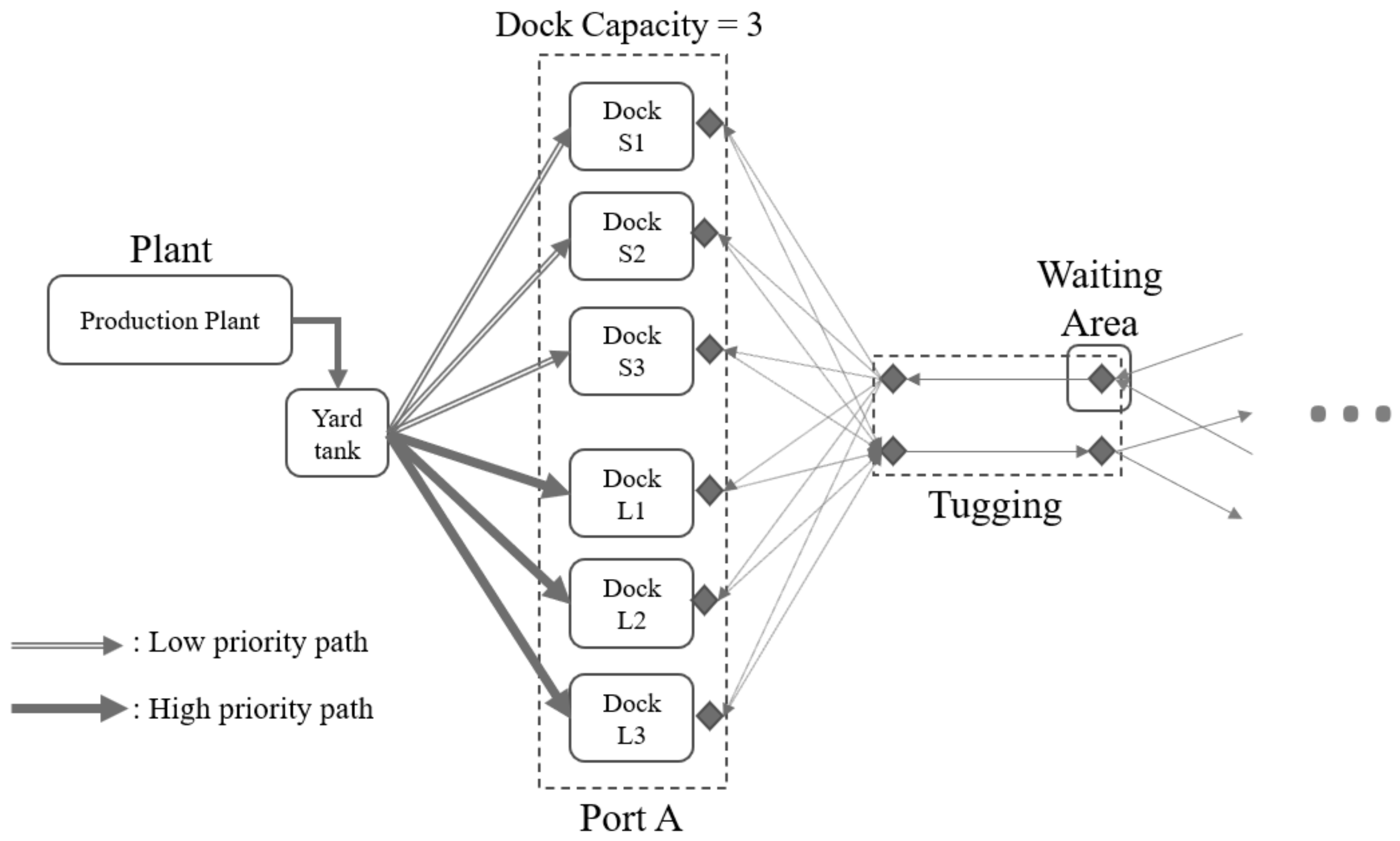
3.1.1. Model Description

We model the proposed problem as a continuous, discrete event simulation model. The product is modeled as a continuous entity, and all other events such as bad weather, vessel, and port operations are modeled as discrete events. A schematic diagram of our developed model is shown in Figure 2 to convey the developed logic clearly. The source, the “Production plant”, creates a metric ton of the products as a continuous entity according to its production rate. The products created in the Production plant leave the system at the “Outflow sink”. Our model employs the transporter module in Simio to simulate vessel operations. Two transporter modules in Figure 2 represent vessels with different capacities (large and small). The model attempts to transport all produced products, making the shipment demand proportional to the production volume. Hence, it operates as a push system.
The product first flows to (and is stored in) the “Yard tank,” which supplies the product to three docks. The movement of the containerized product from the “Yard tank” to three docks is approximately modeled using flow paths. Empty vessels initially wait at the waiting area until a dock becomes available and move through the tugging path to any one of the available docks at the origin port (i.e., Port A). The tugging module only allows one vessel movement for either arrival or departure during a specified duration (i.e., three hours). The first berthed vessel is loaded first under the current FAFU vessel priority policy. If there is a sufficient amount of product in the Yard tank, several vessels can be loaded simultaneously. Once a vessel is fully loaded, it can be tugged if a tugging path is available. Otherwise, the vessel waits at the dock until a tugging path becomes available.
After going through the tugging path, the vessel departs with the destination information and moves to the destination port through the predefined route. Upon arrival at the destination, the vessel may wait some time to be berthed, following the specified distribution at the destination port. On berthing at the terminal of the destination port, the duration of the operation follows the average estimated time (due to a lack of actual data), which includes tie-up, unloading of products, and departure time. After unloading the products, the empty vessel returns to Port A and waits in the waiting area until there is an available dock at Port A. The unloaded entities at the two destination ports are stored in the “Virtual tank” to estimate the amounts of products transported easily and animate the transported volume.
A few unique logic conditions, such as resource restriction, vessel selection, and routing requirements, have been incorporated in the developed model. To implement the resource restriction in the system, we employed two resource modules. The “Dock capacity” resource size is set to be three, representing the number of docks. It is decremented by one whenever a dock is seized (i.e., berthed) by a vessel and incremented whenever released. Therefore, according to the current available room in the Dock capacity, the model determines if another vessel waiting at the waiting area can be berthed or should wait longer. Similarly, the “Tug capacity” resource monitors and allows one vessel in the tugging paths at any time. Hence, only one arriving or departing vessel can move through the tugging paths at a time.
The predefined vessel ranking in the model determines which vessel is tugged to a dock from the waiting area. The destination assignment for each fully loaded vessel is implemented in the routing logic at each dock by randomly assigning a specific destination port using the current cargo volume shipped to each destination: 85% of the products are transported to Port B and 15% to Port C.
The vessel waiting times at the Port A waiting area are controllable by managers. Thus, these values are not entered but are determined by the simulation logic. However, the uncontrollable vessel waiting times at destination Ports B and C are input, following the specified distribution functions fitted to historical data. Furthermore, the voyage times between ports are set to be constants using average values from the assumption that the voyage time between ports is relatively stable. The model also considers the regularly scheduled maintenance time (e.g., six hours every three months) for vessels by using the reliability logic in the transporter module.
The bad weather conditions for high wind and low visibility are modeled as discrete random events following the distribution according to the historical weather data. For example, a high-wind weather entity randomly arrives in the system according to the distribution for interarrivals. Then, it stays in the “High wind” condition during the period specified by the fitted distribution. While the high wind condition is in effect, the vessels are unable to leave port. However, vessels already underway will continue to move to the destination port regardless of the weather condition. Once the high wind condition is cleared, all voyage operations return to normal. The same logic is applied to a low visibility random event with the different distributions for interarrival and duration, using the “Visibility” condition. The bad weather conditions are illustrated in the upper part of Figure 2.
The developed model assesses several performance metrics of the system. It provides details on the amount of product produced and transported, counts the number of trips by each vessel, accounts for operating costs (including voyage and port dues), and estimates GHG emissions. To estimate such performance metrics which are not provided by Simio, several variables are defined as user-defined statistics in the model.
The generation of a simulation model that mimics a real-world situation requires a set of data. The used data have been collected from the internal documents of the studied company, the public weather database, and interviews with field experts. The following is a list of data used in the designing process of the simulation model: production volume; vessel operating times (i.e., voyage and tugging times); loading and unloading times at terminals; vessel capacity, and operating costs (i.e., fuel cost per round trip and port dues). Processes probability distributions are fitted to each of the following processes: vessel waiting at the destination ports; high-speed wind (interarrival time and duration), and low visibility (interarrival time and duration) (see the details in Section 4.2).

3.1.2. Simulation Logic for Large-Vessel-First-Use Policy

Our preliminary analysis estimated the unit fuel cost of a vessel for one round-trip voyage between the origin and destination ports using the average fuel cost per round trip divided by the vessel capacity. Due to the confidentiality of the information, we can only mention that a large vessel has a lower unit fuel cost than a small vessel, indicating that using a large vessel first would reduce the operating cost as proposed by [29]. On the other hand, a small vessel takes less loading and unloading time than a large vessel. Thus, using a small vessel first would more often improve the operational agility of the whole shipping system. Therefore, it would be worthwhile to investigate the impact of using a large vessel first on both operating costs and overall system performance.
The proposed large-vessel-first-use (LVFU) policy requires selecting a large vessel first among all the available vessels in the waiting area. We can implement this relatively easily by assigning a higher ranking to large vessels than small vessels in the list of vessels. In addition, under the LVFU policy, when large and small vessels are loading products simultaneously at the origin port, large vessels should be filled first whenever possible. Because implementing such loading priority control is not trivial, we demonstrate our implementation logic as depicted in Figure 3.
We added six virtual docks to simulate the three physical docks with the LVFU policy. Three docks (S1, S2, and S3) are used only for small vessels, and the other three (L1, L2, and L3) are only used for large vessels. Because the “Dock capacity” resource restricts the number of vessels that can be berthed to be three, only up to three of six virtual docks can be used, making the terminal capacity the same as the three physical docks. Then, by controlling the flow priority on the paths connecting the Yard tank to each dock, three docks for large vessels will prioritize loading products over the other three docks for small vessels. The three paths connected to the same group of docks have equal priority.
We explain the presented logic further using an example. Suppose that two large vessels are berthed at Docks L1 and L2, and one small vessel is berthed at Dock S1. Then, no other vessels can enter the terminal area, and all must wait at the waiting area. When the inventory in the Yard tank is sufficient, large and small vessels can be loaded simultaneously. If the inventory in the Yard tank is not sufficient, products will be supplied from the Yard tank to Dock L1 and L2 first until two large vessels are fully loaded. Then, products will be provided to Dock S1 to load the small vessel. If any one of three vessels finishes loading and departs via a tugging path, then another vessel (large vessel first) at the waiting area can be berthed and begin to load products. The maximum number of vessels berthed is three, and a large vessel will always have a higher priority for loading products. This pattern will be retained continuously throughout the simulation run.

3.1.3. Model Validation

To ensure that the model reflects an actual process, we employ a few procedures to validate its correctness. First, we have developed several other small test models, each of which includes only one specific logic. These test models have been examined by running them step-by-step.
After checking the correctness of the developed logic, the entire model was tested further by simplifying the input data. For example, by using the infinite initial inventory at the origin port, the waiting time of a vessel for products was eliminated. Then, after running the model with such simplified input, several performance measures were examined and compared with the manually calculated estimates. These performance measures include the total amounts of product transported, the total number of trips by each vessel, and the average cycle time for trips.
For example, in the real operating data, the average round-trip time of each type of vessel ranges 52–57 h for a small vessel and 57–62 h for a large vessel. The round-trip times of the tested simulation model were 57–58 h and 62–63 h for small and large vessels, respectively. Even though there is a slight difference, such estimates may be considered sufficiently close, considering variability from weather uncertainty. The developed model is also expected to transport most of the produced products, as happens in the real-port situation. Therefore, we conducted several experiments with different production rates to confirm that the simulation model transported most products with the appropriate number of trips by each vessel as expected.

3.2. Optimization of the Number of Vessels and Travel Speed

This study seeks to find the optimum number of large and small vessels and determine the most economical travel speed to reduce the total costs. The developed optimization model is incorporated into the simulation model to prescribe such decisions while satisfying all the required system constraints. Table 1 defines all notations used in the optimization model.
By using the notations defined in Table 1, we formulate an optimization model as follows.
Minimize z = C R L x L + C R S x S + C P L t L + C P S t S + C V L 2 + S 0 V R   s F 1 + S 0 V R   s B 1 t L + C V S 2 + S 0 V R   s F 1 + S 0 V R   s B 1 t S
Subject to:
y L T
0 x L M N L  
0 x S M N S  
S F l s F S F m  
S F l s B S F m
x L , x S :   integer
s F , s B :   0.1 integer
The objective function (1) is to minimize the sum of three types of costs: rental costs, port dues, and the operating costs of large and small vessels. The first two terms are the rental costs of large and small vessels. The third and fourth terms are port dues of large and small vessels. The last two terms are the voyage costs, which are the sum of the forward and backward voyage costs. The voyage cost is a function of the number of trips and speed factors. A speed factor ( s F and s B ) of 1.0 means the speed at S0.
Constraint (2) restricts the amount of product transported to be at least the target volume. Constraints (3) and (4) impose the possible range of the number of large and small vessels, respectively. Constraint (5) specifies the range of the forward speed factor, and Constraint (6) specifies the range of the backward speed factor. Constraints (7) and (8) invoke integer restrictions on decision variables. Note that the decision variables s F and s B have discrete values with a step size of 0.1.

3.3. Environmental Impact

The proposed operating policy must care about GHG emissions while being cost-efficient. Therefore, carbon dioxide (CO2) and sulfur dioxide (SO2) emissions are estimated and compared with the current system emissions. The emission factors of CO2 and SO2 for marine diesel oil and the method of calculating the total emissions in this study are adopted from [30]. Their method requires multiplying the fuel consumption of a vessel by the emission factors of CO2 and SO2. Detailed calculations using the data are provided in Section 5.5. Estimating the environmental effects according to the fuel consumption is a typical technique in transportation systems, as shown in [31].

4. Numerical Study

This section provides numerical studies to assess the performance of the proposed operating policies. The study investigates the optimal number of each type of vessel and forward and backward voyage speeds using the developed simulation model.

4.1. Design of Experiments

We designed experiments under two different vessel priority policies, FAFU and LVFU, as shown in Table 2. Columns #LV and #SV mean the number of large and small vessels used, respectively. Case C0 represents the current operating condition, in which two large and two small vessels are utilized at the constant voyage speed of 22.2 km/h (12 knots). The first four cases (C0, C1, C2, and C3) used the FAFU policy for vessel priority, and the other four cases (C4, C5, C6, and C7) used the LVFU policy. The simulation model ran for one year with 20 replications. The OptQuest simulation optimization engine was used for the optimization model with the following parameters: default replications: 10, max replications: 30, max scenarios: 3000, confidence level: 0.95, and relative error of the confidence level: 0.05.
Case C1 uses the same number of vessels as case C0. It investigates the impact of the lower voyage speed determined by the optimization model by examining the forward speed (FS) and backward speed (BS) factors with a decrement of 0.1 from 1.0 to 0.7. Speed factor 0.7 represents 70% (15.6 km/h) of the current speed (22.2 km/h), and speed factor 1.6 represents 160% (35.6 km/h) of the current speed. In case C2, the optimization model determines the number of each type of vessel while the speed factors remain constant at the current operating speed. Our preliminary tests to transport most of the produced products determined the ranges for the number of each type of vessel (i.e., 0~3 for #LV and 0~4 for #SV).
In particular there may be a trade-off between the number of vessels and voyage speed, such that a higher voyage speed may need a smaller number of vessels and vice versa. Thus, we designed case C3 to find the optimal number of each type of vessel and optimal speed factors simultaneously, considering the FS and BS factors from 0.7 to 1.6. Cases C4–C7 have the same structure as cases C0–C3 except that they follow the vessel priority policy of LVFU.

4.2. Data

Table 3 and Table 4 summarize the data collected from the practical working conditions used in the simulation model. However, due to the confidentiality of the information, the cost values in Table 4 are replaced by symbols. The production rate in the model was set at 8,901 metric tons per day by taking the average value of the real production rate. In particular, the waiting times at Ports B and C are estimated as the gamma distribution, which is fitted to the limited historical data.
According to the field experts who manage the system studied in this research, wind speeds greater than 35 km per hour and low visibility of less than 1 km are the stopping conditions for vessel operations. We collected the wind-speed and visibility–distance hourly data from 2014 to 2019 from the world weather online database (World Weather Online) [32]. From the collected historical data, we extracted the interarrival time and duration of high-speed wind (>35 km/h) and low visibility (<1 km). Table 5 shows the distributions fitted to the extracted data.
The best-fitted distribution for the interarrival times of both high-speed wind and low visibility is the Weibull distribution. The beta distribution is weakly fitted to the duration data of high-speed wind and low visibility. We employed the beta distribution for those rather than using an experimental distribution to reduce simulation runtime.
This study also estimates CO2 and SO2 emissions as a performance metric of environmental effect. The total amounts of CO2 and SO2 emissions are calculated by multiplying the emission factors of CO2 or SO2 by the fuel consumption. According to Wei and Zhao (2010), the emission factors of CO2 and SO2 are 3,179 g/kg marine diesel oil and 7 g/kg marine diesel oil, respectively.

5. Results and Discussions

This section presents and analyzes the results of our numerical studies from five different analytical perspectives.

5.1. Impact of Lowering Voyage Speed with the Current Number of Vessels

Table 6 provides the results of lowering voyage speed with the current number of vessels (two large and two small vessels) on the system performance. The column “Product volume” gives the produced amounts and transported amounts of products in metric kilo-tonnes (KT). The column “Costs” provides total cost and cost breakdown, including rental cost, port dues, and voyage cost. In case C1, the forward and backward speed factors are decision factors determined by the optimization model. Table 6 also includes the results of some examined cases for the voyage speed factors to identify a meaningful pattern.
Within the considered range of the speeds, all cases could transport more than the target volume (3248 KT), which is 99% of the produced product. As the forward and backward speeds decrease, the total costs decrease proportionally due to lower fuel consumption. The lowest speed with the FS factor of 0.7 and BS factor of 0.7 is the most economical, saving 11% (1,125,620 USD per year) compared with the total cost of case C0. However, there is no meaningful difference between lowering forward and backward speeds: the cost reduction from reducing 0.1 of the FS factor is similar to that obtained by lowering the BS factor by the same amount.

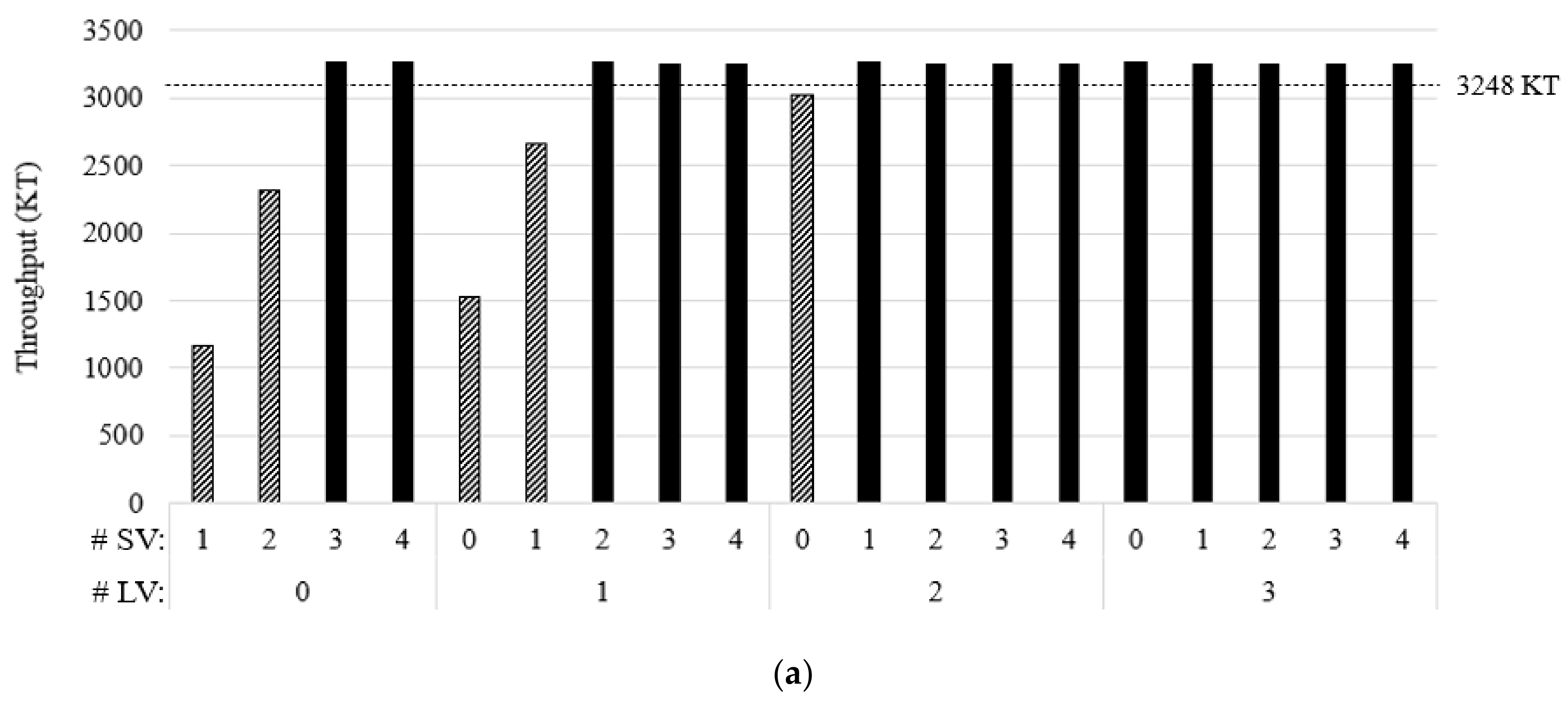
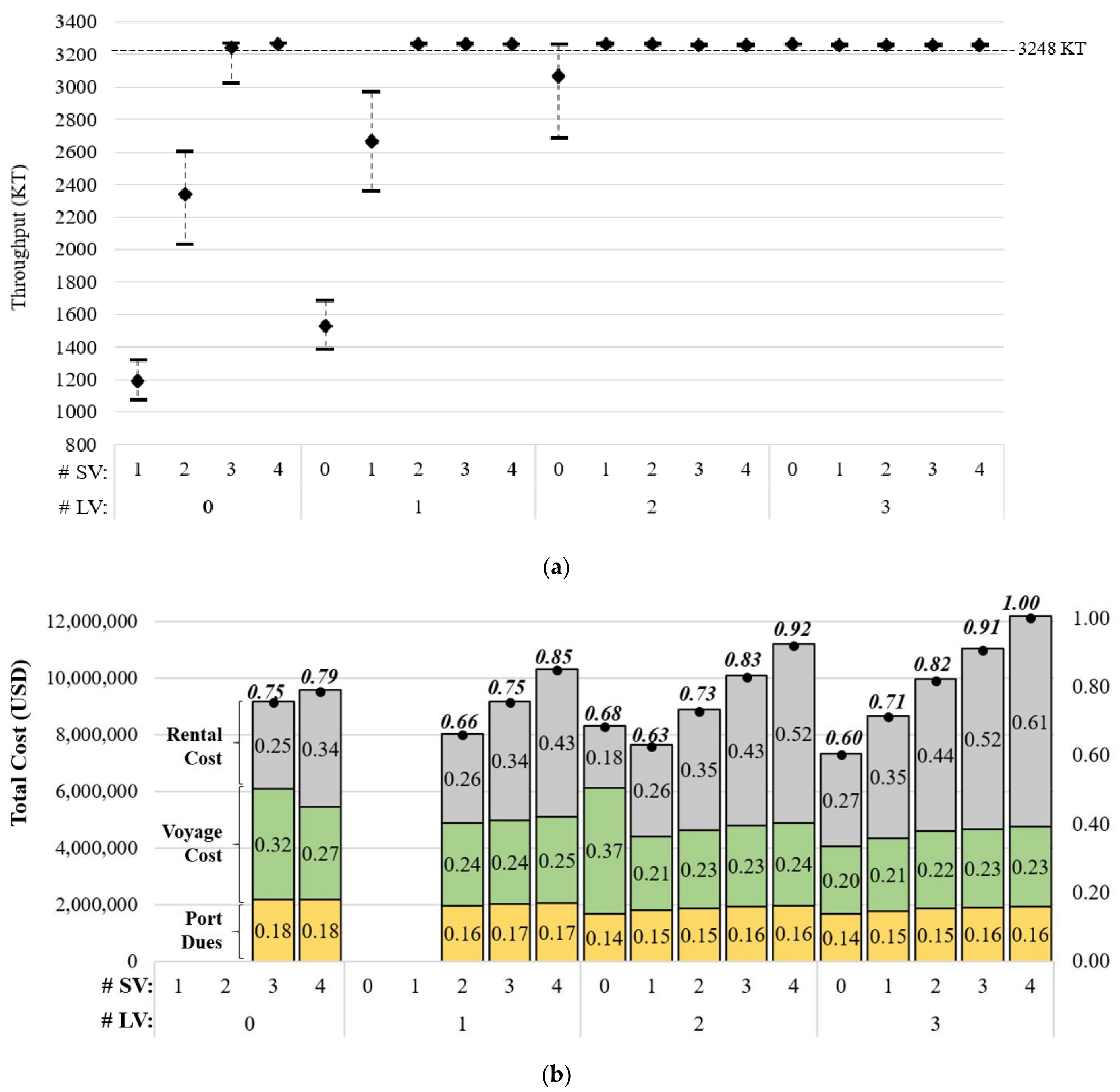
5.2. Impact of the Number of Vessels at the Current Voyage Speed under FAFU

Figure 4 illustrates the results of case C2, in which the optimization model determines the number of each type of vessel at the current travel speed. #LV in Figure 4 represents the number of large vessels, and #SV is that of small vessels. Figure 4a shows the system throughput, which is equivalent to the transported volume per year. A few cases could not meet the target throughput (3248 KT). Either three large vessels or small vessels could transport the target product volume. As one fewer large vessel is used, one more small vessel is needed to meet the throughput target.
In addition, we analyze the cost breakdown structure of case C2 as shown in Figure 4b only for the feasible cases that meet the target throughput. The left y-axis is the total cost, and the right y-axis is the ratio of the total cost of each case of large and small vessels to the highest total cost when (#LV, #SV) = (3, 4).
In most cases, the port dues ratios are similar and vary slightly from 0.13 to 0.16. Port dues decrease slightly as the number of large vessels increases. Total dues decrease because a large vessel needs fewer trips than a small vessel to transport the same amount of products. Similarly, the voyage cost decreases slightly as the number of large vessels increases because a large vessel has a lower unit voyage cost than a small vessel.
However, the rental cost of a large vessel is larger than that of a small vessel. Thus, as the number of large vessels increases, the rental cost increases. There is a trade-off between the operating cost (voyage cost and port dues) and rental cost according to the number of large and small vessels. The smallest total cost occurs when only three large vessels and no small vessels are used, that is, (#LV, #SV) = (3, 0). From the result, we infer a large vessel’s economic benefit from saving voyage cost and port dues may be better than the disadvantage from the increasing rental cost under the considered cost structure.

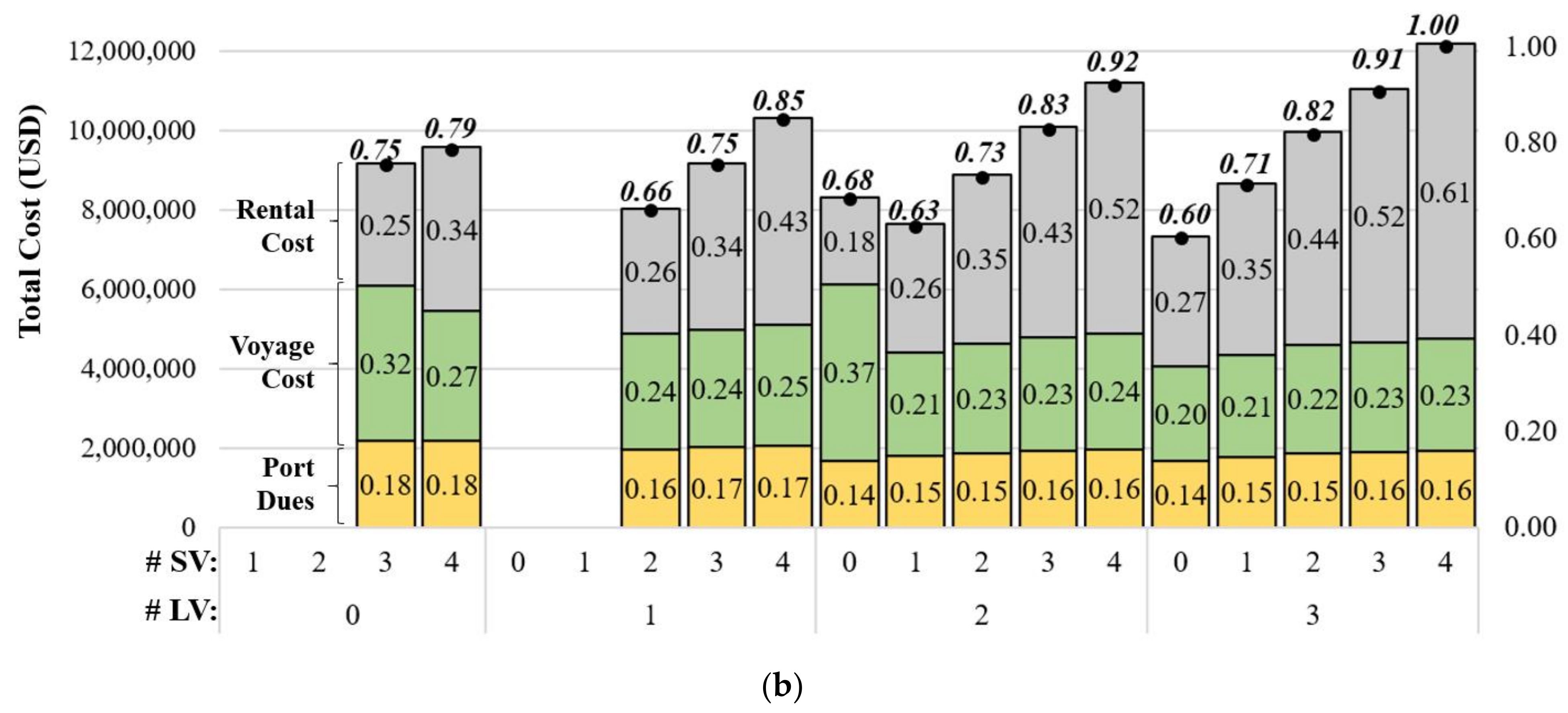
5.3. Impact of the Number of Vessels and Voyage Speeds under FAFU

In case C3, the number of each type of vessel and forward and backward voyage speed factors are decision variables. Even though the optimization model gives the optimal solutions, we investigate the entire range of solution space to obtain insight into the decision factors.
For the given numbers of each type of vessel, the voyage speed factors may or may not affect the throughput. Such a pattern is illustrated in Figure 5a. It shows the minimum, maximum, and average amounts of the transported products. When the number of vessels is not sufficient: (#LV,#SV) = (0,1), (0,2), (1,0), (1,1), even higher travel speeds cannot transport the target product volume. At the same time, when the number of vessels is sufficient, the travel speed does not affect the throughput. However, when the number of vessels is tight: (#LV,#SV) = (0,3), (2,0), the target transportation volume can be achieved only at high voyage speeds.
Figure 5b shows the cost breakdown at the optimal travel speed for the number of each type of vessel. The smallest total cost is acquired when (#LV, #SV) = (3,0), which is the same as case C2. The variation in the port dues is also relatively minor, such as in case C2 (see Figure 4b). However, when (#LV,#SV) = (0,3) and (2,0), the portions of the voyage cost are 0.32 and 0.37, respectively, which are higher than that of other numbers of vessels (0.20~0.27). This outcome is because only high speeds could meet the target throughput when (#LV,#SV) = (0,3) and (2,0), incurring higher fuel consumption than other, lower-speed cases.

5.4. Best Solutions and Impact of LVFU

Finally, Table 7 summarizes the best solutions for each case. In the columns #Vessel and Speed factor, the underscored values mean that they are decision factors and have been prescribed as the best solutions by the optimization model. Several subcolumns under “Costs” provide detailed information for the economic performance metrics. The total cost is the sum of the rental and operating (voyage cost and port due) costs. Column Saving gives the cost savings from the difference between the total costs of case C0 and the case in each row. Column Saving (%) is calculated by the cost-saving of each case divided by the total cost of case C0. The undercored values in #Vessel and Speed Factor mean that they are prescribed by the optimization model.
In case C4, we applied the LVFU policy using the current number of vessels and speed. The LVFU policy shows potential for a cost saving of 1.2% (125,200 per year) compared to case C0. All such cost saving is from the savings in the operating costs. In case C5, which also utilizes two large and two small vessels, the optimization model prescribed the same speed factors as case C1 (0.7 for the FS factor and 0.7 for the BS factor). Case C5 could show a slight cost saving of 0.2% compared to case C1. The cost savings by applying the LVFU policy are 1.2% from case C0 to C4 at the current voyage speed and 0.2% from case C1 to C5 at the lowest voyage speed. We infer that lowering the voyage speed may provide less opportunity to select a large vessel from the idle vessels in the waiting area by making most vessels travel slowly somewhere in the system.
However, the optimal number of vessels in case C6 is the same as that in case C2. Moreover, case C7 has the same optimal number of vessels and speed factors as case C3. The LVFU policy has not affected any results of cases C6 and C7 because the optimal solutions for cases C6 and C7 use three large vessels only, making no difference between FAFU and LVFU.
Overall, cases C3 and C7 generated the same best results among all cases tested, saving 26.8% (2,692,410 USD/year) of total costs compared with case C0. The number of vessels and speed factors significantly affected the total costs. The LVFU policy has a limited effect when the number of large and small vessels is mixed and the voyage speed is not slow. However, the LVFU policy is still a recommendable operating option because it can be adopted easily for practical operations.

5.5. Environmental Effect

Table 8 presents the detailed performance metrics of all cases about the number of trips by each type of vessel, fuel consumption in metric tons (T), GHG emissions in metric tons (T), and % reduction compared with case C0. The GHG emissions are directly converted from the marine diesel oil consumption using the conversion factors described in Section 4.2. Lowering the voyage speed reduces the fuel consumption significantly up to around 30% (see cases C1 and C5). Moreover, utilizing large vessels more also shows good environmental benefits by reducing GHG emissions by 14% (see cases C2 and C6). Finally, our proposed optimal solutions reduce the GHG emissions up to 39% compared with case C0 (see cases C3 and C7).
In particular, by applying the LVFU policy in case C4, GHG emissions could be reduced 2% compared with case C0. Even though the large vessel’s fuel consumption per trip is greater than a small vessel’s, the total number of trips could be reduced by using large vessels more often under the LVFU policy. Accordingly, the total fuel consumption could be decreased. However, as the voyage speeds are lowered in cases C1 and C5, the impact of the LVFU policy on GHG emissions becomes smaller. It may be related to the inference discussed in Section 5.4 that slowing voyage speeds may let most vessels travel slowly somewhere, reduce the vessels idling in the waiting area, and lower the chance of selecting a large vessel from those. From cases C6 and C7, we do not see the impact of the LVFU policy as only large vessels are utilized.

5.6. Larger Production Volumes for Future Scenarios

The studied company has a plan to increase its production capacity in a few years. Thus, it would be valuable to examine larger production volume cases. Table 9 presents three additional test cases and results for double (C8), triple (C9), and quadruple (C10) production volumes using the LVFU policy. The prescribed number of vessels and speed factors in cases C8 and C9 show a similar pattern to the current production volume: (1) only large vessels are utilized, and (2) the lowest speed is best.
However, in case C10, the model could not find any solution to transport more than 99% of the produced products to the destinations even with a sufficient number of vessels. The current capacity of the plant-side port (i.e., three docks) is not sufficient to handle such a large transportation volume, making many vessels wait to enter the port. Thus, to quadruple the production volume, the company should invest not only in its manufacturing facilities and vessels but also in the port infrastructure to accommodate more vessels.

6. Conclusions

The present study has successfully developed a simulation model for a closed-loop vessel shipping system considering various uncertainties from weather and uncontrollable delays at destination ports. Furthermore, the developed optimization model embedded in the simulation model prescribes the optimal number of each type of vessel and forward and backward voyage speeds to minimize the total costs. To the best of our knowledge, this is the first simulation and optimization study to address the proposed closed-loop vessel dispatching problem. Further, we have devised a new vessel-use priority policy (LVFU) and compared it with the current policy (FAFU).
The numerical studies showed that the optimal solution prescribed uses only three large vessels at the lowest voyage speed to transport the target product volume. It could save 26.8% (2,692,410 USD/year) of the total cost and reduce GHG emissions up to 39% compared with the current operating condition. Lowering voyage speed showed a significant impact on system performance. Additionally, a large vessel has good economic benefits from saving the voyage cost and port dues, which are greater than the disadvantage of the increased rental fee. Furthermore, even though the LVFU policy has a moderate effect, it would still be a recommendable operating option to be used with the current number of vessels and travel speed. The larger volume test results indicate that quadruple production volume may require additional investment on the plant-side port to accommodate more vessels.
The present study provides a useful insight and decision-support tool for industrial managers to determine the most economical and environmentally friendly operating conditions for a closed-loop vessel shipping system. The structure of the considered logistics system from the manufacturing facility at a coastal area to a hub port for long-distance transportation can be found easily in many energy and heavy industries around the world. Thus, the presented modeling concept and approach may be applicable to many business cases in other countries. The fruitful contribution of this study could be strengthened by further work that may integrate the production plant maintenance schedule and dynamic vessel speed optimization in every trip.

Author Contributions

Conceptualization, H.A.; methodology, H.A. and F.B.; software, H.A. and F.B.; validation, H.A. and F.B; formal analysis, H.A. and F.B.; investigation, H.A. and F.B.; resources, H.A. and F.B.; data curation, H.A. and F.B.; writing—original draft preparation, H.A. and F.B.; writing—review and editing, H.A., F.B., and D.-W.L.; visualization, H.A., F.B. and D.-W.L.; supervision, H.A.; project administration, H.A.; funding acquisition, H.A. All authors have read and agreed to the published version of the manuscript.

Funding

This work was supported by Khalifa University of Science and Technology [RC2 DSO].

Institutional Review Board Statement

Not applicable.

Informed Consent Statement

Not applicable.

Conflicts of Interest

The authors declare no conflict of interest.

References

  1. Perkins, R.; Malek, M.; Perkins, R. Middle East Refinery, Petrochemicals Output to Surge by 2040: IEA; S&P Global Platts: London, UK, 2010. [Google Scholar]
  2. Perera, L.P.; Mo, B. Ship speed power performance under relative wind profiles in relation to sensor fault detection. J. Ocean Eng. Sci. 2018, 3, 355–366. [Google Scholar] [CrossRef]
  3. Karan, C. 10 Important Points Ship’s Officer on Watch Should Consider during Restricted Visibility; Marine Insight: Bangalore, India, 2018. [Google Scholar]
  4. World Meteorological Organization. Guide to Marine Meteorological Services; no. 471; World Meteorological Organization: Geneva, Switzerland, 2018.
  5. Pruzan-Jorgensen, P.M.; Farrag, A. Sustainability Trends in the Container Shipping Industry: A Future Trends Research Summary; Business for Social Responsibility Report; Business for Social Responsibility: New York, NY, USA, 2010. [Google Scholar]
  6. Paris, C. Clouds hover over shipping’s key antipollution law. Wall Str. J. 2018. Available online: https://www.wsj.com/articles/clouds-hover-over-shippings-key-antipollution-law-1541002430 (accessed on 11 October 2021).
  7. Joung, T.-H.; Kang, S.-G.; Lee, J.-K.; Ahn, J. The IMO initial strategy for reducing Greenhouse Gas(GHG) emissions, and its follow-up actions towards 2050. J. Int. Marit. Safety Environ. Aff. Shipp. 2020, 4, 1–7. [Google Scholar] [CrossRef] [Green Version]
  8. Bergh, I. Optimum speed—from a shipper’s perspective. DNV Contain. Ship Update 2010, 2, 10–13. [Google Scholar]
  9. Cheng, L.; Duran, M.A. Logistics for world-wide crude oil transportation using discrete event simulation and optimal control. Comput. Chem. Eng. 2004, 28, 897–911. [Google Scholar] [CrossRef]
  10. Merrick, J.R.W.; Van Dorp, J.R.; Dinesh, V. Assessing Uncertainty in Simulation-Based Maritime Risk Assessment. Risk Anal. 2005, 25, 731–743. [Google Scholar] [CrossRef]
  11. Franzese, L.; Fioroni, M.; Paz, D.; Botter, R.; Gratti, C.; Martinez, A.; Bacigalupo, C. Supply-chain simulation and analysis of petroleum refinery systems: A reusable template with incremental approach. In Proceedings of the Winter Simulation Conference, Monterey, CA, USA, 3–6 December 2006. [Google Scholar]
  12. Almaz, A.; Altiok, T. Simulation modeling of the vessel traffic in Delaware River: Impact of deepening on port performance. Simul. Model. Pract. Theory 2012, 22, 146–165. [Google Scholar] [CrossRef]
  13. Kulak, O.; Polat, O.; Gujjula, R.; Günther, H. Strategies for improving a long-established terminal’s performance: A simulation study of a Turkish container terminal. Flex. Serv. Manuf. J. 2011, 25, 503–527. [Google Scholar] [CrossRef]
  14. Ilati, G.; Sheikholeslami, A.; Hassannayebi, E. A Simulation-Based Optimization Approach for Integrated Port Resource Allocation Problem. Promet Traffic Transp. 2014, 26, 243–255. [Google Scholar] [CrossRef]
  15. Carotenuto, P.; Giordani, S.; Zaccaro, A. A Simulation Based Approach for Evaluating the Impact of Maritime Transport on the Inventory Levels of an Oil Supply Chain. Transp. Res. Procedia 2014, 3, 710–719. [Google Scholar] [CrossRef] [Green Version]
  16. Rahimikelarijani, B.; Abedi, A.; Hamidi, M.; Cho, J. Simulation modeling of Houston Ship Channel vessel traffic for optimal closure scheduling. Simul. Model. Pr. Theory 2018, 80, 89–103. [Google Scholar] [CrossRef]
  17. Lababidi, H.; Ahmed, M.; Alatiqi, I.; Al-Enzi, A. Optimizing the supply chain of a petrochemical company under uncertain operating and economic conditions. Ind. Eng. Chem. Res. 2004, 43, 63–73. [Google Scholar] [CrossRef]
  18. Saharidis, G.K.; Minoux, M.; Dallery, Y. Scheduling of loading and unloading of crude oil in a refinery using event-based discrete time formulation. Comput. Chem. Eng. 2009, 33, 1413–1426. [Google Scholar] [CrossRef]
  19. Oliveira, F.; Hamacher, S. Optimization of the Petroleum Product Supply Chain under Uncertainty: A Case Study in Northern Brazil. Ind. Eng. Chem. Res. 2012, 51, 4279–4287. [Google Scholar] [CrossRef]
  20. Nishi, T.; Izuno, T. Column generation heuristics for ship routing and scheduling problems in crude oil transportation with split deliveries. Comput. Chem. Eng. 2014, 60, 329–338. [Google Scholar] [CrossRef]
  21. He, J.; Huang, Y.; Chang, D. Simulation-based heuristic method for container supply chain network optimization. Adv. Eng. Inform. 2015, 29, 339–354. [Google Scholar] [CrossRef]
  22. Ghezavati, V.; Ghaffarpour, M.; Salimian, M. A hierarchical approach for designing the downstream segment for a supply chain of petroleum production systems. J. Ind. Syst. Eng. 2015, 8, 1–17. [Google Scholar]
  23. Ye, Y.; Liang, S.; Zhu, Y. A mixed-integer linear programming-based scheduling model for refined-oil shipping. Comput. Chem. Eng. 2017, 99, 106–116. [Google Scholar] [CrossRef]
  24. Aydin, N.; Lee, H.; Mansouri, S. Speed optimization and bunkering in liner shipping in the presence of uncertain service times and time windows at ports. Eur. J. Oper. Res. 2017, 259, 143–154. [Google Scholar] [CrossRef] [Green Version]
  25. An, H.; Choi, S.; Lee, J.H. Integrated scheduling of vessel dispatching and port operations in the closed-loop shipping system for transporting petrochemicals. Comput. Chem. Eng. 2019, 126, 485–498. [Google Scholar] [CrossRef]
  26. Bahamaish, F.; Al-Mutawa, S.A.; Sumaidaa, M.F.; An, H. Simulation modeling of the closed-loop vessel scheduling for petrochemical products. In Proceedings of the IISE Annual Conference, Orlando, FL, USA, 18–21 May 2019. [Google Scholar]
  27. An, H.; King, N.; Hwang, S.O. Issues and solutions in air-traffic infrastructure and flow management for sustainable aviation growth: A literature review. World Rev. Intermodal Transp. Res. 2019, 8, 293–319. [Google Scholar]
  28. An, H. Optimal daily scheduling of mobile machines to transport cellulosic biomass from satellite storage locations to a bioenergy plant. Appl. Energy 2019, 236, 231–243. [Google Scholar] [CrossRef]
  29. Tran, N.K.; Haasis, D.H. An empirical study of fleet expansion and growth of ship size in container liner shipping. Int. J. Prod. Econ. 2015, 159, 241–253. [Google Scholar] [CrossRef]
  30. Wei, Q.; Zhao, S. Estimating CO2 Emission and Mitigation Opportunities of Wanzhou Shipping in Chongqing Municipality, China. In Proceedings of the International Conference on Logistics Engineering and Intelligent Transportation Systems, Wuhan, China, 26–28 November 2010; pp. 1–4. [Google Scholar]
  31. An, H.; Byon, Y.-J.; Cho, C.-S. Economic and Environmental Evaluation of a Brick Delivery System Based on Multi-Trip Vehicle Loader Routing Problem for Small Construction Sites. Sustainability 2018, 10, 1427. [Google Scholar] [CrossRef] [Green Version]
  32. World Weather Online. Available online: https://www.worldweatheronline.com/ (accessed on 30 September 2021).
Figure 1. Schematic structure of the studied closed-loop vessel dispatching system.
Applsci 11 09626 g001
Figure 2. Schematic diagram of the simulation model for the closed-loop vessel shipping system.
Applsci 11 09626 g002
Figure 3. Simulation logic for LVFU policy.
Applsci 11 09626 g003
Figure 4. Impact of the number of vessels at the current voyage speed under FAFU (case C2): (a) transported volume; (b) cost breakdown.
Applsci 11 09626 g004aApplsci 11 09626 g004b
Figure 5. Impact of the number of vessels and voyage speeds under FAFU: (a) transported volume; (b) cost breakdown at the optimal travel speeds.
Applsci 11 09626 g005
Table 1. Notations for the optimization model.
Indices
i = L, S (L: large vessel, S: small vessel)
k = B, F (B: backward, F: forward)

Parameters
C P i : port dues per trip of type i vessel
C R i : rental cost per year of type i vessel
C V i : voyage cost per one-way trip of type i vessel at speed S0
L T : minimum target of throughput (transported amount per year)
M N i : maximum number of type i vessel
S 0 : current speed (22.2 km/h (12 knots))
S F l : minimum value of speed factor (0.7)
S F m : maximum value of speed factor (1.3)
V R : voyage cost change rate per voyage speed (4.3% per km/h (8% per knot))

Decision variables
s k : speed factor, integer*0.1
x i : the number of type i vessels, integer

Outcomes
t i : the number of trips per year by type i vessel
y : throughput (transported amount per year)
z: total cost per year
Table 2. Design of experiment.
Case#LV#SVVessel PriorityVoyage Speed Factor
FSBS
C022FAFU11
C122FAFU0.7~1.0 (*)0.7~1.0 (*)
C20~3 (*)0~4 (*)FAFU11
C30~3 (*)0~4 (*)FAFU0.7~1.6 (*)0.7~1.6 (*)
C422LVFU11
C522LVFU0.7~1.0 (*)0.7~1.0 (*)
C60~3 (*)0~4 (*)LVFU11
C70~3 (*)0~4 (*)LVFU0.7~1.6 (*)0.7~1.6 (*)
(*): decision factor.
Table 3. Time duration for operations.
LocationOperationsTime (h)
Small VesselLarge Vessel
ATugging for arrival33
Loading1216
Tugging for departure33
SeaVoyage A<->B18 (=9 × 2)18 (=9 × 2)
Voyage A<->C22 (=11 × 2)22 (=11 × 2)
B, CWaiting at B, C2 + Gamma(3.86, 1.43)
(shape: 3.86, scale: 1.43)
2 + Gamma(3.86, 1.43)
(shape: 3.86, scale: 1.43)
Unloading at B, C1416
Table 4. Vessel information.
TypeSmall VesselLarge Vessel
Number22
Capacity in the specification (TEU)650950
Current utilized max capacity (t)744410,880
Average fuel cost per round trip (USD)ab
Port dues (USD)cd
Table 5. High-speed wind and low visibility data and fitted distribution.
# Data PointsMeanStd dev.Distribution ExpressionSquare Errorp-Value
High-speed WindInterarrival time (day)6230.152.20.999 + Weibull (12, 0.38)
(Scale: 12, Shape: 0.38)
0.0018<0.005
Duration (hour)632.762.50.5 + 15*Beta (0.544, 3.07)
(alpha: 0.544, beta: 3.07)
0.00710.238
Low VisibilityInterarrival time (day)4334.959.80.999 + Weibull (5.76, 0.259)
(Scale: 5.76, Shape: 0.259)
0.0016<0.005
Duration (hour)445.52.930.5 + 12*Beta (1.4, 1.9)
(alpha: 1.4, beta: 1.9)
0.02930.213
Table 6. Impact of lowering voyage speed with the current number of vessels.
CaseNoVoyage Speed FactorProduct Volume (KT)Costs (USD/Year)
FSBSProducedTransportedTotal CostRental CostPort DuesVoyage Cost
C0-113274.833259.3210,020,6004,258,3301,889,7203,872,540
C1110.93274.833260.309,836,7004,258,3301,890,2403,688,120
20.913274.833258.929,839,4404,258,3301,891,1203,689,990
310.83274.833258.129,639,2104,258,3301,886,6803,494,200
40.813274.833259.679,643,2804,258,3301,887,8403,497,110
510.73274.833260.589,450,0804,258,3301,885,4803,306,270
60.713274.833260.709,445,4404,258,3301,883,9603,303,150
70.90.93274.833257.899,648,8304,258,3301,889,7203,500,780
80.80.83274.833257.959,261,1004,258,3301,884,2203,118,550
90.70.73274.833258.188,894,9804,258,3301,886,0802,750,570
Table 7. Comparison of vessel selection rule from the best results of all cases.
CaseVessel
Priority
#VesselSpeed FactorProduct Volume
(KT/Year)
Costs (USD/Year)
LVSVFSBSProducedTransportedTotalSavingSaving (%) *RentalOperating
C0FAFU22113275.2326210,034,800--4,258,3305,776,450
C4LVFU22113275.232639,909,600125,2001.2%4,258,3305,651,270
C1FAFU220.70.73275.232618,892,0901,142,71011.4%4,258,3304,633,750
C5LVFU220.70.73275.232658,866,3101,168,49011.6%4,258,3304,607,980
C2FAFU30113275.232648,306,5201,728,28017.2%3,285,0005,021,520
C6LVFU30113275.232648,306,5201,728,28017.2%3,285,0005,021,520
C3FAFU300.70.73275.232647,342,3902,692,41026.8%3,285,0004,057,390
C7LVFU300.70.73275.232647,342,3902,692,41026.8%3,285,0004,057,390
*: Saving (%) = 100 × (Total cost of C0 − Total cost of the case)/Total cost of C0.
Table 8. Fuel consumption and GHG emissions.
CaseVessel Priority#VesselSpeed Factor#TripsMarine Diesel Oil Consumption (T)Emissions (T)Reduction (%) *
LVSVFSBSLVSVLVSVTotalCO2SO2
C0FAFU221116819025892741563217,90339-
C4LVFU221119015929242285550317,494392%
C1FAFU220.70.717318318921882398812,6762829%
C5LVFU220.70.718017419711781396312,6002830%
C2FAFU3011299-4596-485615,4373414%
C6LVFU3011299-4596-485615,4373414%
C3FAFU300.70.7299-3272-345710,9912439%
C7LVFU300.70.7299-3272-345710,9912439%
*: Reduction (%) = (Fuel consumption of C0 − Fuel consumption of the case)/Fuel consumption of C0.
Table 9. Large production volume cases.
Case#LV#SVVessel PriorityVoyage Speed FactorProduct Volume (KT)#VesselSpeed Factor
FSBSProducedTransportedLVSVFSBS
C80~60~8LVFU0.7~1.60.7~1.666036580500.70.7
C90~90~12LVFU0.7~1.60.7~1.699049860800.70.7
C100~120~16LVFU0.7~1.60.7~1.612,942-----
Publisher’s Note: MDPI stays neutral with regard to jurisdictional claims in published maps and institutional affiliations.

