Profit-Driven Methodology for Servo Press Motion Selection under Material Variability

Abstract

Servo presses enable new types of forming motion profiles that can be used to stamp difficult materials, such as high strength steels. This paper presents an application of Bayesian statistics to intelligently select which motion profile maximizes the expected utility given the properties of the incoming material. Bayesian logistic regression was used in conjunction with expected utility to estimate manufacturing returns, which can be used to make informed process decisions. A use case is presented, which demonstrates that the Smart Forming Algorithm can increase expected returns by more than 20%.

1. Introduction

In the last 15 years, industry has begun adopting servo presses as a replacement for conventional presses in metal forming. Servo presses enable the press motion profile to be designed for improved forming results. Of particular interest for this work, new high strength steels with applications for vehicle lightweighting can be successfully formed with servo motion [1]. However, high strength steels are known to have a relatively wide variability in material properties [2]. This variability can lead to inconsistent results from a designed servo motion profile.

Since good parts can be sold for profit and defective parts induce a loss, it is important, when planning for profits, to consider the uncertainty of what kind of parts will be produced. This paper proposes a Bayesian statistical tool in helping manufacturers estimate returns in the face of uncertainty.

A typical metal forming manufacturing process begins with a roll of sheet metal arriving at the manufacturer. The metal is rolled out through a press, where the metal is stamped into a specified shape. Although servo presses allow for variations in press motion, a simple manufacturing approach is to let the press run one pre-configured motion. After the part comes out of the press, it can be examined for defects. If the part is found to have no defects, it is good to be assembled for a final product and provides value. Defective parts are scrapped and induce a loss (Figure 1). Here, a part is considered defective if a forming expert identifies cracking, necking, or wrinkling during a visual inspection. The proposed Smart Forming Algorithm fits into the process after the metal blank or coil arrives but before it is stamped (Figure 2). As the metal is rolled into the press, sensors can detect material properties of the metal and relay that information to a software application running the Smart Forming Algorithm. The Smart Forming Algorithm then produces probability distributions of producing a good part for several press motions. Employing these probabilities in expected utility can provide recommendations to the operator as to which press motion is expected to produce the greatest number of good parts.

Returning to the simple approach of using one pre-configured press setting, one strategy of making a profit is to choose the press setting that produces the greatest number of good parts based on previously collected data. However, this approach could be improved, as press motions can yield different results even when the material properties of the input sheet metal are similar. Although, ideally, suppliers would produce sheet metal with consistent material properties, the reality is that material properties vary across batches, even from the same supplier.

The proposed Smart Forming Algorithm is a framework for taking both press motion and material property variability into account when predicting the probability that the part produced will be good. Applying the theory of expected utility to the Smart Forming Algorithm can then provide profit estimates. The manufacturer can use these estimates to make an informed decision in its strategy to make a profit. The proof-of-concept work presented here suggests that manufacturers can expect to achieve substantial cost savings as smart forming approaches are generalized for wider application.

2. Previous Work

Various techniques have been used to monitor, model, optimize, and control servo press motion to minimize defects [3,4,5,6,7]. As an example of the benefits and key considerations when designing a press motion profile, pulse motion named JIM-FORM was developed for improved deep draw forming. The pulse motion allows lubrication to re-flow between the die and the surface allowing a higher drawing height. However, pulse motion also increases the cycle time [8]. As a second example of the importance of carefully designing the motion profile, it has been shown that the press motion can be designed to avoid strain path failures [9].

Current solutions to improving good part production rates typically use an iterative approach known as metamodeling, wherein (1) simulations are run in search of an optimal parameter setting, (2) a part is then produced based on the simulations results, and (3) the actual results are incorporated into optimal parameter searching for another round of simulations and actual runs [10,11,12] (see also Yang et al. [13], for an additive manufacturing example). More recent work adopts neural networks in place of traditional simulations within the metamodeling process [14] (see also Zimmerling et al. [15], for a textile forming example; for machine learning more generally within manufacturing, see [16,17]). The work most similar to what is presented here developed a Bayesian framework to predict variables within a full production line [18]. Like other previous work, it was interested in building accurate but quickly computed data to replace simulation, ultimately to be used in line with production. The proposed Smart Forming Algorithm is a simpler Bayesian model and does not attempt to replace simulation. It is instead focused on helping make inline process decisions.

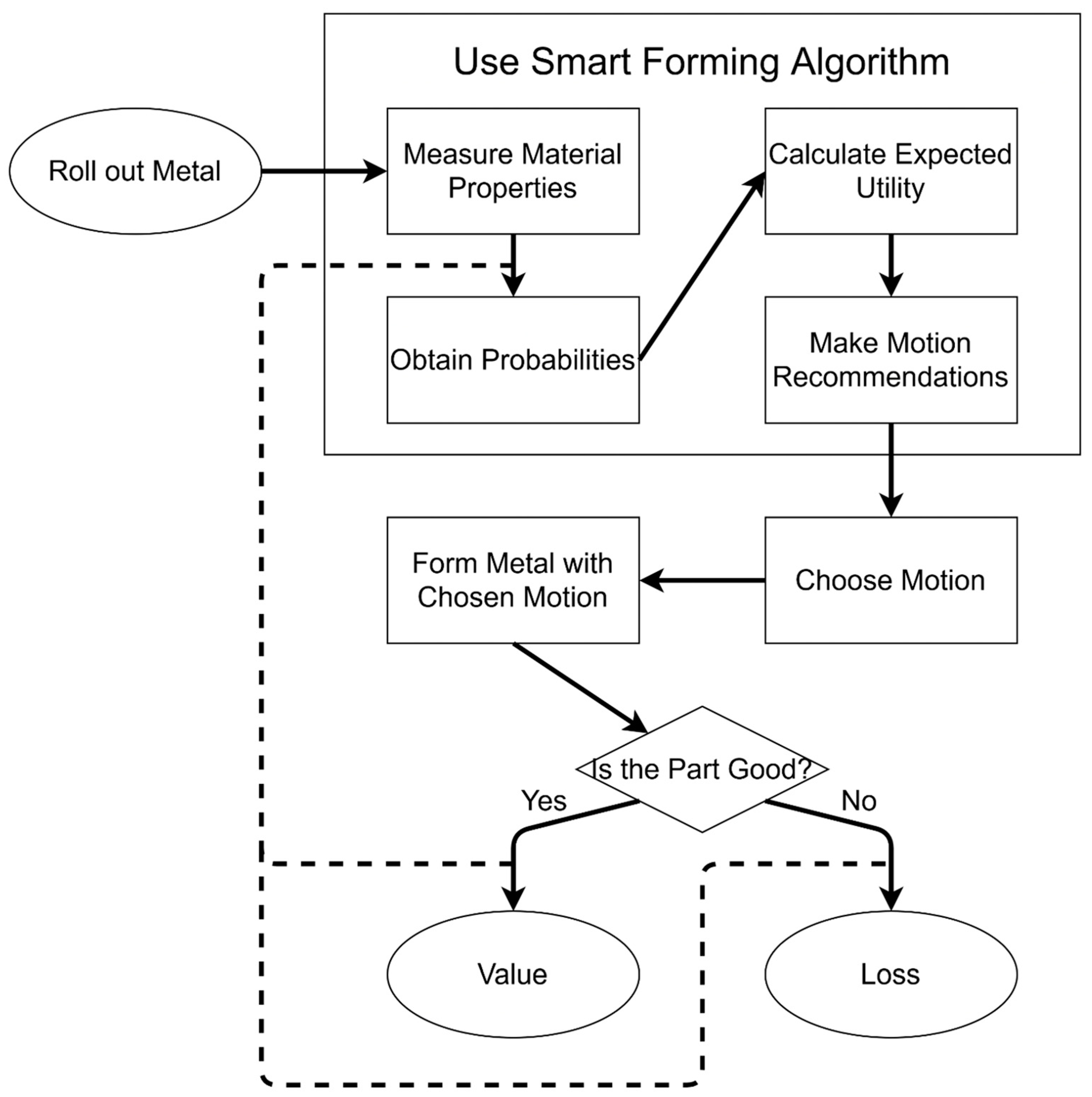
3. Smart Forming Algorithm

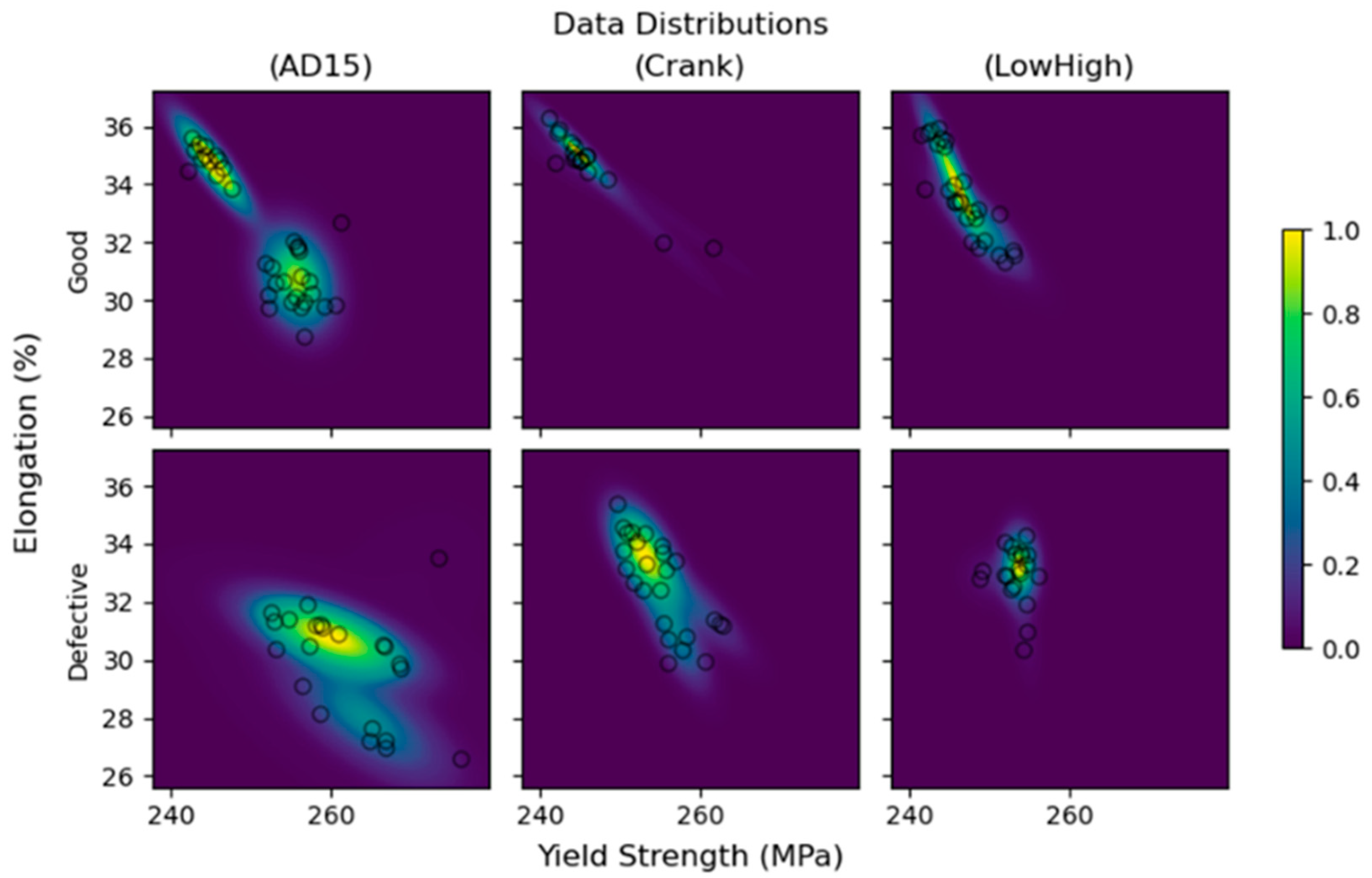
At its core, the Smart Forming Algorithm trains a Bayesian Logistic Regression that takes yield strength and elongation data as inputs and outputs the probability of a part being good. (Although in general, the yield strength of a material is correlated with its elongation, it is not perfectly correlated. Initial investigations showed that yield strength and elongation were less correlated to each other than they were to tensile strength. In fact, it was only after ignoring tensile strength that model training reached convergence). One regression is trained for each press motion. Once each of these sub-models is trained, the model can answer the question, “What is the probability of a part being good given X press motion, and an input metal with Y yield strength and Z elongation?”.

Bayesian statistical models, such as the one used in the Smart Forming Algorithm, begin with prior probability distributions, which are parameterized with initial model parameters. As data are included for inference, the posterior distribution can be sampled from with Markov Chain Monte Carlo (MCMC). While the posterior distribution may not have a recognizable form with parameters, Bayesian inference nevertheless works on the basis that the prior distributions (or the assumed probability distributions) are updated as more data become available. In this way, the initial model parameters act as a starting belief, which is updated according to the data.

3.1. Data

The data used to train the Smart Forming Algorithm in this paper were from forming experiments that were conducted on three batches of 0.75 mm thick BH340 steel [19]. A 3MA system was used to measure the magnetic properties of a sample of the input sheets, after which ASTM E8/E8M-16a (Specimen 1 in Table 13 of ASTM E8/E8M-16a) tensile tests were performed on the measured material to calibrate the magnetic response. A quasistatic strain rate of 0.008 s⁻¹ was used for the uniaxial tensile testing. Three different orientations, 0°, 45°, and 90° with respect to the rolling direction, were selected for tensile testing. This approach was found to be reliable in past works [20]. The calibration data were used to calculate the material properties of subsequent sheets. Those sheets were then stamped according to a variety of press motions. Finally, the resulting parts were evaluated either as a good part or not.

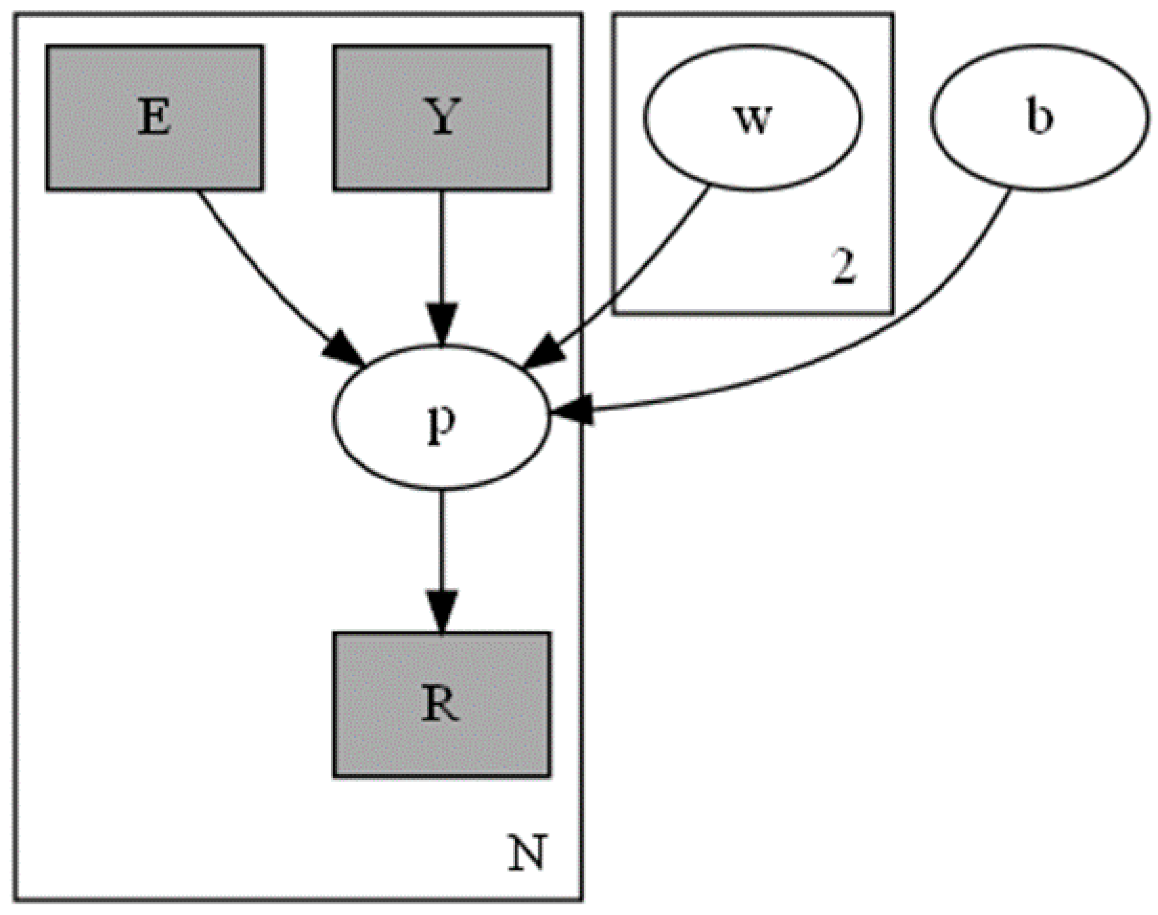
3.2. Bayesian Logistic Regression

Bayesian Logistic Regression is a Bayesian formulation of Logistic Regression, which is the classical machine learning approach to predicting the probability of an outcome given feature information [21]. In other words, Bayesian Logistic Regression not only provides the probability of an outcome, it also provides an uncertainty for the predicted outcome.

The graphical model (Figure 3) shows a representation of the Bayesian Logistic Regressions trained for the Smart Forming Algorithm. (Note that Figure 3, which is a probabilistic graphical model, should not be confused with a block diagram of a closed-loop feedback system). “E” refers to elongation, “Y” refers to yield strength, “w” refers to weights applied to terms, “b” refers to an intercept term, “p” refers to the probability of a part being good, and “R” refers to the observed outcome. As the plate notation shows, the model learns from N data points, and there are two weighted terms. The model parameters are related in the following way:

$$w_i~N\left(0,{10}^3\right),i\in \left\{1,2\right\}$$

(1a)

$$b ~ \mathrm{Uniform}(-\infty ,\infty )$$

(1b)

$$p_j=w_1{E}_j+w_2{Y}_j+b,j\in \left\{1,2,\dots ,N\right\}$$

(1c)

$$R_j~\mathrm{Bernoulli}\left(p_j\right),j\in \left\{1,2,\dots ,N\right\}$$

(1d)

In other words, each weight has a prior of a normal distribution centered at 0 and with standard deviation of 1000, b has a completely uninformative prior, p is a linear combination of E and Y, and R is distributed as a Bernoulli with probability p.

Data standardization (subtraction of sample mean and division by sample standard deviation) is applied to yield strength and elongation, respectively. Training is accomplished by MCMC to probabilistically estimate the model’s parameters based on training data consisting of yield strength, elongation, and outcome (i.e., whether the part was good or defective) for a particular press motion. PYMC3 was used to build and train the model by MCMC [22] (see also [23] for a descriptive example of the implementation of Bayesian logistic regression using PYMC3).

Note that by design, model parameters are not shared across different press motions because it was expected that each press motion could exhibit different outcomes, even on metals with similar material properties. The Smart Forming Algorithm trained sub-models for three different press motions: “Crank”, “LowHigh”, and Attach–Detach 15 mm (which is referred to as “AD15”). Details on these motions can be found in previous work [19]; in summary, Crank is the conventional method for metal forming; LowHigh is Crank with adjustments to the blank holder force during the stroke; and AD15 is an advanced motion of the servo press. (Tests were implemented with a 300-ton AIDA servo press. The final drawing depth was set to be 68.8 mm for most testing conditions. Fuchs Anticorit PL 39 LV 12 was uniformly applied on the blank surfaces before the test using the motorized roller application equipment, UNIST. The Crank motion is a simple stamping motion applied with a blank holder force of 150 kN, while LowHigh is Crank motion with an adjustment to the blank holder force from 100 kN to 150 kN during the stroke. Figure 4 illustrates the AD15 motion from the bottom dead center. The press ram changes its moving directions during drawing the blank under a constant BHF. The intermediately drawn part does not release from the die and binder during the slide detach while the drawn top surface is separated with the stationary bottom punch that makes local springback possible and creates new contact points with the punch at the second-stroke drawing [19]). Since training with MCMC took roughly a minute per press motion, this model is not ideal for real-time updating in a metamodel approach. However, each of the trained model parameters can be saved for later reuse, allowing for real-time prediction.

Using the model’s prediction capabilities for whether a good part is produced for a particular yield strength, elongation, and press motion, decision plots can be made (Figure 5). Since the model provides uncertainty estimations in its predictions, an upper and lower bound can be given on the prediction, by calculating the Highest Density Interval (HDI) for a given percentage. For the results presented, 68.27% was used, as that is the probability of choosing a random value within one standard deviation of the mean of a normal distribution. For simplicity, the HDI calculation was constrained so that the interval would be continuous. (A more accurate but complex HDI could be discontinuous, as would be the case where the distribution has two peaks on the extremes and a valley in the center).

Plotting this information was accomplished using matplotlib (Figure 5). The circles and crosses represent measured data points, placed according to their yield strength and elongation. The coloring of the top row reflects the model’s expected probability of a good part. Each point in the 500 × 500 grid of yield strength and elongation was queried against the model for the specified motion profile. The coloring of the bottom row reflects the difference between the upper and lower bounds of the credibility interval. Again, a 500 × 500 grid was used as query points against the appropriately trained model. Upper and lower bounds were computed according to the HDI parameters specified earlier.

The first thing to note about the decision surfaces is where the good parts (circles) and the defective parts (crosses) tend to be. As expected, each motion produced good parts at different ranges. For example, AD15 managed to make good parts in the yield strength range of 250–262 with elongation range of 28–31.5%, although it showed some variations. Meanwhile, in the same range, Crank seemed to get mostly defective parts, and LowHigh had few data points. On the other hand, they all consistently produced good parts when yield strength was in the 240–245 range, and elongation was in the 33–36% range (upper left corners).

The decision surfaces (top plots) indicate how the expected probability of a good part increased or decreased depending on material properties. Yellow (light) indicates higher probability of a good part, while purple (dark) indicates lower probability of a good part. Based on the top plots, the models learned the relationship between material properties and part quality reasonably well, as the circles tend to be in the yellow regions and the crosses tend to be in the purple regions. The transition regions between yellow and purple in these top plots indicate a change from lower to higher (or higher to lower) probability. It is expected that for each plot, the change from yellow to purple follows a line, as the Bayesian Logistic Regression used a linear relationship to predict good part probabilities.

The interval width surfaces (bottom plots) indicate the difference between the upper and lower bound probabilities for a particular point in the material properties space. Lighter regions indicate a wider interval between the upper and lower bounds calculated by the models, while darker regions indicate a narrower interval. As expected, the lighter regions tend to be around the regions where probabilities change from lower to higher (or higher to lower).

These decision surfaces show some of the strengths and weaknesses in the Bayesian Logistic Regression approach used in this paper. All the top plots are yellow along the left, which means the models learned that good parts tend to come from metal with lower yield strength. This makes sense, given the cluster of good parts that all plots show in the upper left region. Unfortunately, the models seem not to have learned to put boundaries on how far out good parts can be: the interval width plots are purple for most of the good parts region, indicating that the models are very certain about metals with arbitrarily low yield strength to come out good. This is due to the linear assumption made by the Bayesian Logistic Regression used in this paper. A more sophisticated method that could allow for non-linear relationships might be able to restrict high certainty of good parts regions to around the circles instead of extrapolating out indefinitely. (A Bayesian Logistic Regression with a non-linear kernel function was tested along with the linear version presented in this paper. Unfortunately, the non-linear version tended to overfit to the training data, causing even more problematic regions of high certainty. For example, the non-linear Crank model had high certainty that good parts could come from the right region, likely due to overfitting on the good parts that appear among the defective parts. On the other hand, the non-linear LowHigh model learned to have high certainty of high probabilities in what appeared to be an oval-shaped region around the blue dots. There was also a large region of low certainty along the bottom. These ideal patterns probably arose as a result of LowHigh’s blue dots tending not to mingle with red dots).

3.3. Expected Utility

Expected utility theory provides a framework for making decisions under uncertainties [24]. The core calculation to make decisions requires quantification of uncertainties for the context in which a decision is made. The Smart Forming Algorithm can provide such uncertainty quantities in the form of probabilities for part quality given press motion and material properties of input metal. For the problem of choosing an appropriate press motion for a given batch of metal, expected utility can calculate expected returns for each press motion with the given batch of metal if it is also given estimates for good part profit and defective part loss. In addition, the number of parts produced by a given motion in a particular amount of time can be accounted for, thus leading to estimates for the expected returns over a length of time.

4. Use Cases

4.1. Expected Profits

As an example of using the Smart Forming Algorithm with expected utility, consider the following problem. Suppose that α, the profit from a good part, equals USD 2, and that γ, the loss from a defective part, equals USD 3. Given an hour to run, AD15 can yield 1538 parts, while Crank and LowHigh can yield 2000 parts. Now suppose a batch of metal comes in with a yield strength of 255 MPa and an elongation of 30%. The expected profit/loss for each press motion within that hour can be estimated with the help of expected utility.

The expected utility of each motion can be calculated as follows:

$$EU\left(m\right)=\alpha \ast N_m\ast P\left(o=1|m,255,30\right)-\gamma \ast N_m\ast P(o=0|m,255,30)$$

(2)

In the equation, m refers to the press motion, $N_m$ refers to the number of parts produced by motion m in an hour, $P\left(o=1|m, 255, 30\right)$ refers to the probability of the part being good given that motion m was used on a metal with yield strength 255 MPa and elongation 30%, and $P(o=0|m, 255, 30)$ refers to the probability of the part being defective under the same conditions.

Because the Smart Forming Algorithm returns a distribution of probabilities for a good part being produced, upper and lower bound probabilities can be easily obtained. The Smart Forming Algorithm’s expected probability of good part production is estimated by taking the median of the probabilities sampled by MCMC. (Technically, the expected value of an empirical distribution created from the MCMC samples should be the mean of the sampled values. However, because MCMC samples converge to the correct distribution after an infinite number of samples, values that are highly unlikely may still get into the finite sample collection, skewing the mean. To avoid this problem, the median was chosen as an estimation of the expected probability of a good part being produced. This also ensured that the expected probability lay within the lower and upper bounds computed by the continuous HDI). Using this process, the following numbers can be obtained, where the expected return is given first and the parenthesized values show the lower bound expected return and the upper bound expected return:

• AD15: +USD 844.62 (+USD 205.55, +USD 1847.48);
• Crank: −USD 5999.99 (−USD 5999.99, −USD 5999.98);
• LowHigh: −USD 1294.92 (−USD 5999.27, +USD 1360.05).

The expected return bounds for Crank are quite narrow, indicating that the model is quite certain about defective parts from Crank. The expected return bounds for LowHigh, however, are far apart. This indicates that the model is uncertain about how probable LowHigh is to produce good parts, though it expects that the parts are more likely to be defective. AD15 manages to remain positive not only in expected returns but also in both bounds.

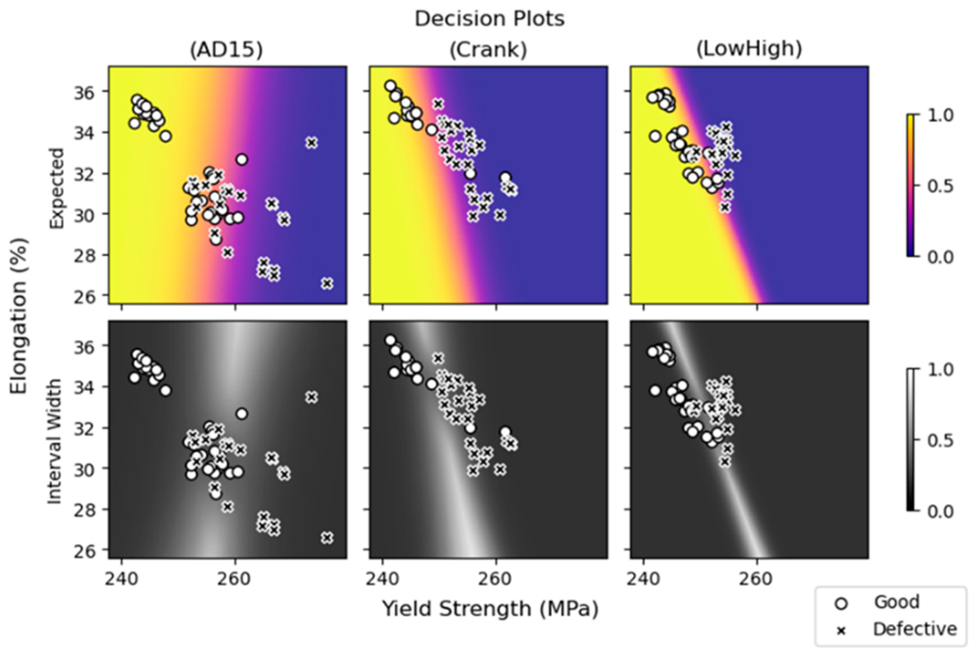
4.2. Preferred Strategy for Press Motion Selection

To investigate the effect of expected utility theory in action, a simulation was developed. The simulation assumes a year of production with 2800 working hours. For each hour, a batch of metal comes in with some yield strength and elongation. Four options are available to the operator: AD15, Crank, LowHigh, and Downtime. The first three options correspond with using the press motion with the same name for that batch, while Downtime is the decision to produce nothing that hour and wait for the next batch of metal.

To simulate a production-relevant distribution of material, multiple mixtures of Gaussians were trained on the data (Figure 6) to create a data model. One mixture of Gaussian was trained for every combination of motion and outcome (i.e., good part or defective part). Data points were sampled from each mixture of Gaussian such that the samples were distributed as the distribution of the full data set. One data point was collected for each simulated hour. This plot was created using the Python matplotlib package. The measured data points were used to model a Bayesian Gaussian mixture with five components with the scikit-learn package in Python.

The results of the simulation repeated 1000 times (

Table 1. Expected Utility Predictions.

Strategy	Returns	Good Parts	Total Parts
AD15	3.940 (+/− 0.090)	3.372 (+/− 0.018)	4.306 (+/− 0.000)
Crank	−5.058 (+/− 0.170)	2.348 (+/− 0.034)	5.6 (+/− 0.000)
LowHigh	−4.299 (+/− 0.187)	2.500 (+/− 0.037)	5.6 (+/− 0.000)
Smart Forming	6.097 (+/− 0.063)	3.597 (+/− 0.029)	3.963 (+/− 0.029)

Note: Values are reported in millions of USD and arbitrarily truncated at the third decimal place for readability. AD15, Crank, and LowHigh refer to the strategy of using the named press motion exclusively, on every batch. The Smart Forming strategy employs expected utility with expected probabilities from the Smart Forming Algorithm to choose an appropriate press motion based on the material properties of incoming metal. Mean and standard deviation values are reported, rounded to the thousands place. For example, the AD15 strategy has a mean expected return of about USD 3.94 million over all simulation runs, and the standard deviation of the returns over all simulation runs was about USD 90,000. The winning strategy is Smart Forming, which had a mean expected return of USD 6.097 million.

) show expected utility values in the case of the following strategies: (1) always choose AD15, (2) always choose Crank, (3) always choose LowHigh, and (4) use the Smart Forming Algorithm’s expected values with expected utility. Expected utility with the Smart Forming Algorithm is the winning strategy, with a mean expected return of about USD 6.097 million over all 1000 simulation runs. The losing strategy was Crank, with a mean expected loss of USD 5.058 million.

It may be surprising that the Smart Forming Algorithm could beat AD15 in expected returns when the other motions had negative expected returns. One factor that allows the Smart Forming Algorithm to beat AD15 is the number of parts that each motion produces per hour. Recall that AD15 produces fewer parts per hour than Crank or LowHigh. Thus, if a batch of metal arrives from which all three methods are equally likely to produce a good part, it would be better to choose Crank or LowHigh, as they will produce more good parts than AD15 in the same amount of time. Another factor is the flexibility to choose a motion that is most likely to produce a good part. For example, if a metal comes in that LowHigh has a higher probability of producing a good part than Crank and AD15, then LowHigh can be used for that hour. A final factor in the Smart Forming Algorithm’s ability to beat AD15 is the choice to not produce anything. When the probability of a good part is so low that the current metal will not produce enough good parts to offset the loss of the defective parts, it would be better to stop production and wait for the next batch rather than take the loss from the defective parts.

4.3. Flagging Model Uncertainty

Because of the Bayesian basis of the model, uncertainty in model prediction can be detected and used advantageously. Suppose that a batch of metal comes in with a yield strength of 257 MPa and an elongation of 26%, and AD15 was chosen as the press motion. According to the decision plots (Figure 5), the AD15 model is uncertain of the probability of a good part being produced (the region is yellow in the bottom plot). The Smart Forming Algorithm could raise an indicator to the operator to pay extra attention to the parts produced. If defective parts start coming out, the operator can halt production to stop further losses.

5. Summary and Conclusions

This paper presented a Bayesian model that accounts for the uncertainty of a formed part being good, given a press motion as well as the yield strength and elongation properties of the input sheet metal. Combined with the theory of expected utility, this model not only provides revenue estimates for using a particular motion but also recommends a motion strategy to maximize profits.

The future of this model is promising. An important next step will be the generalization of this proof-of-concept model for different presses, designs, materials, and failures modes. We expect additional sensor modalities, such as lubrication sensors and thickness sensors, and the use of simulations will play a large part in generalizing this approach and broadly realizing the value of this approach. Further, the model could be generalized to continuously modify servo motion parameters rather than selecting from a series of pre-determined motion profiles.

Another change potentially worth investigating is incorporation of raw 3MA data in place of material property data. Since material properties are measured by a calibrated device, the model may become more accurate by using the raw sensor measurements instead of the material properties calculated by the calibrated device. Finally, the method used to generate data in the optimal strategy case study could be integrated with the model to advise users when the model is extrapolating to a data point far from the training data.

Of course, the wisdom of experienced operators should not be ignored. The model is a tool to help operators and manufacturers make more informed press setting decisions. Grounded in Bayesian statistics, the model is not a replacement for experts and laborers. Rather, it is a framework to aid in thinking about what motion to use when presented with a batch of sheet metal.

References

1. Mori, K.-I. Application of Servo Presses to Sheet Metal Forming. Key Eng. Mater. 2011, 473, 27–36. [Google Scholar] [CrossRef]
2. Tisza, M. Development of Lightweight Steels for Automotive Applications. In Engineering Steels and High Entropy-Alloys; IntechOpen: London, UK, 2020. [Google Scholar] [CrossRef] [Green Version]
3. Yang, M. Smart metal forming with digital process and IoT. Int. J. Lightweight Mater. Manuf. 2018, 1, 207–214. [Google Scholar] [CrossRef]
4. Lai, C.F.; Wong, H.I.; Ng, C.H.; Yahaya, S.N.M.; Shamsudin, S. Review on Acoustic Emission Monitoring System for Hot Stamping Process. In Recent Trends in Manufacturing and Materials towards Industry 4.0; Springer: Singapore, 2021. [Google Scholar] [CrossRef]
5. Kim, S.Y.; Kubota, S.; Okuda, M. Detection of Abnormal Behavior in Manufacturing Processes Using Bolt Type Piezo-Sensor. In Proceedings of the 68th Japanese Joint Conference for the Technology of Plasticity, Fukui, Japan, 9–12 November 2017. [Google Scholar]
6. Allwood, J.M.; Duncan, S.R.; Cao, J.; Groche, P.; Hirt, G.; Kinsey, B.; Kuboki, T.; Liewald, M.; Sterzing, A.; Tekkaya, A.E. Closed-loop control of product properties in metal forming. CIRP Ann. 2016, 65, 573–596. [Google Scholar] [CrossRef] [Green Version]
7. Barthau, M.; Liewald, M. New approach on controlling strain distribution manufactured in sheet metal forming components during deep drawing process. In Proceedings of the International Conference on the Technology of Plasticity, ICTP 2017, Cambridge, UK, 17–22 September 2017. [Google Scholar]
8. Tamai, Y.; Yamasaki, Y.; Yoshitake, A.; Imura, T. Improving Deep Drawability of Steel Sheets by Motion Control of Servo Press-Development of New Forming Technology with Servo Press. J. Jpn. Soc. Technol. Plast. 2010, 51, 450–454. [Google Scholar] [CrossRef] [Green Version]
9. Zoller, L.; Feister, T.; Kim, H. The Effects of Servo Press Forming on Various Strain Path Failures. In Forming the Future; Springer: Cham, Switzerland, 2021; pp. 2829–2836. [Google Scholar] [CrossRef]
10. Bonte, M.; Boogaard, A.H.V.D.; Huetink, H. A Metamodel Based Optimisation Algorithm for Metal Forming Processes. In Advanced Methods in Material Forming; Springer: Cham, Switzerland, 2007; pp. 55–72. [Google Scholar] [CrossRef] [Green Version]
11. Heingärtner, J.; Fischer, P.; Harsch, D.; Renkci, Y.; Hora, P. Q-Guard–an intelligent process control system. In Journal of Physics: Conference Series; IOP Publishing: Bristol, UK, 2017. [Google Scholar]
12. Kumar, S.P.; Lee, S.-S. Meta-model Based Approach to Minimize the Springback in Sheet Metal Forming. Int. J. Mech. Syst. Eng. 2017, 3, 3:IJMSE-121. [Google Scholar] [CrossRef] [Green Version]
13. Yang, Z.; Eddy, D.; Krishnamurty, S.; Grosse, I.; Denno, P.; Lopez, F. Investigating Predictive Metamodeling for Additive Manufacturing. In Proceedings of the International Design Engineering Technical Conferences and Computers and Information in Engineering Conference, Charlotte, NC, USA, 21–24 August 2016. [Google Scholar] [CrossRef]
14. Lindemann, B.; Jazdi, N.; Weyrich, M. Anomaly detection and prediction in discrete manufacturing based on cooperative LSTM networks. In Proceedings of the 2020 IEEE 16th International Conference on Automation Science and Engineering (CASE), Virtually, Hong Kong, 20–21 August 2020. [Google Scholar] [CrossRef]
15. Zimmerling, C.; Poppe, C.; Kärger, L. Estimating Optimum Process Parameters in Textile Draping of Variable Part Geometries—A Reinforcement Learning Approach. Procedia Manuf. 2020, 47, 847–854. [Google Scholar] [CrossRef]
16. Lindamood, L.R.; Mohr, L.; Moghaddas, A.; Kitt, A.; Frech, T. Investigation of monitoring methods for ultrasonic metal welding. In Sensors and Smart Structures Technologies for Civil, Mechanical, and Aerospace Systems 2021; Society of Photo-Optical Instrumentation Engineers (SPIE): Bellingham, WD, USA, 2021. [Google Scholar] [CrossRef]
17. Finamor, F.P.; Wolff, M.A.; Lage, V.S. Prediction of forming limit diagrams from tensile tests of automotive grade steels by a machine learning approach. IOP Conf. Series Mater. Sci. Eng. 2021, 1157. [Google Scholar] [CrossRef]
18. Havinga, J.; Mandal, P.K.; Boogaard, T.V.D. Exploiting data in smart factories: Real-time state estimation and model improvement in metal forming mass production. Int. J. Mater. Form. 2019, 13, 663–673. [Google Scholar] [CrossRef] [Green Version]
19. Kim, H.; Gu, J.C.; Zoller, L. Control of the servo-press in stamping considering the variation of the incoming material properties. IOP Conf. Ser. Mater. Sci. Eng. 2019, 651, 012062. [Google Scholar] [CrossRef]
20. Alamos, F.J.; Gu, J.C.; Kim, H. Evaluating the Reliability of a Nondestructive Evaluation (NDE) Tool to Measure the Incoming Sheet Mechanical Properties. In Forming the Future; Springer: Cham, Switzerland, 2021; pp. 2573–2584. [Google Scholar] [CrossRef]
21. Bishop, C. Pattern Recognition and Machine Learning; Springer: New York, NY, USA, 2006. [Google Scholar]
22. Salvatier, J.; Wiecki, T.V.; Fonnesbeck, C. Probabilistic programming in Python using PyMC3. PeerJ Comput. Sci. 2016, 2, e55. [Google Scholar] [CrossRef] [Green Version]
23. Coyle, B.; Cook, J.B. GLM: Logistic Regression. 2018. Available online: https://docs.pymc.io/pymc-examples/examples/generalized_linear_models/GLM-logistic.html (accessed on 30 September 2021).
24. Briggs, R. Normative Theories of Rational Choice: Expected Utility. In The Stanford Encyclopedia of Philosophy, Fall 2019 Ed.; Zalta, E.N., Ed.; Available online: https://plato.stanford.edu/archives/fall2019/entries/rationality-normative-utility/ (accessed on 30 September 2021).
Figure 1. Example of parts manufactured by metal forming. Note that the defective part has both a crack as well as wrinkling, though either would be sufficient to classify the part as defective.
Applsci 11 09530 g001
Figure 2. Process diagram of metal forming with the Smart Forming Algorithm. The process diagram without the Smart Forming Algorithm would jump directly from “Roll out metal” to “Choose motion”.
Applsci 11 09530 g002
Figure 3. Graphical model of Bayesian Logistic Regression. The Smart Forming Algorithm trains one such model for each motion.
Applsci 11 09530 g003
Figure 4. Attach–detach slide motion with 15 mm offset from bottom dead center.
Applsci 11 09530 g004
Figure 5. Decision plots for the Smart Forming Algorithm. The top row displays expected probabilities of a good part for a given value of yield strength and elongation. The bottom row displays the difference between the upper and lower bound of the credibility interval, according to a Highest Density Interval (HDI) probability of 68.27%, at each point in the material properties space. Columns correspond to press motion, and good (circles) a defective (crosses) training data points are displayed on each plot.
Applsci 11 09530 g005
Figure 6. Distributions of training data for different press motions. Columns represent press motion, rows separate good and defective data points, circles show training data points, and the coloring is based on the probabilities predicted by a Gaussian Mixtures model.
Applsci 11 09530 g006