Dwell Time Estimation of Import Containers as an Ordinal Regression Problem

Featured Application

Knowing the departure date of each container is paramount to scheduling an optimal stacking in container terminals, and thus, reducing the fuel consumption of the yard cranes. Supervised classification algorithms are typical for estimating such a dwell time. However, we show that an ordinal regression algorithm outperforms the supervised classification algorithms regarding the mean absolute error and the reshuffles generated. This research has been applied in an inbound yard from Cuba as part of a project for the optimization of the import container flow. Our results can state a baseline for further dwell time estimation systems.

Abstract

The optimal stacking of import containers in a terminal reduces the reshuffles during the unloading operations. Knowing the departure date of each container is critical for optimal stacking. However, such a date is rarely known because it depends on various attributes. Therefore, some authors have proposed estimation algorithms using supervised classification. Although supervised classifiers can estimate this dwell time, the variable “dwell time” takes ordered values for this problem, suggesting using ordinal regression algorithms. Thus, we have compared an ordinal regression algorithm (selected from 15) against two supervised classifiers (selected from 30). We have set up two datasets with data collected in a container terminal. We have extracted and evaluated 35 attributes related to the dwell time. Additionally, we have run 21 experiments to evaluate both approaches regarding the mean absolute error modified and the reshuffles. As a result, we have found that the ordinal regression algorithm outperforms the supervised classifiers, reaching the lowest mean absolute error modified in 15 ($71\%$) and the lowest reshuffles in 14 ($67\%$) experiments.

1. Introduction

Optimization problems arise during the operations of stacking containers in the yard of a terminal [1]. One of those is the container Storage Space Allocation Problem (SSAP), a particular case of the storage location assignment problem [2,3,4,5]. SSAP consists of finding the best allocation for each container in a yard minimizing a criterion such as the number of container reshuffles or the crane traveling distance [6]. Operators store arrival containers in multi-level stacks to save storage space using yard cranes. Only containers at the top are accessible by yard cranes. Reaching intermediate containers of the stacks provokes reshuffles. Then, a reshuffle is an unproductive movement of the crane due to inadequate allocation of some containers [5,6].

To reduce the reshuffles, operators need to know a priori the dwell time of each arriving container. The dwell time of a container measures the days (hours or weeks) that it shall stay in the yard [7]. We shall refer to dwell time as the dwell time of import containers in a yard of a container terminal. Predominantly, the actual dwell time is unknown because the departure date to its client depends on several attributes [8]. Thus, operators employ their expertise or some algorithms to estimate the dwell time. By reducing the reshuffles, container terminals lessen their operation time and fuel consumption.

Two approaches are commonly used for estimating the dwell time. The first is an empirical approach based on the operators’ knowledge [9,10,11,12,13]. The second is an approach based on statistical and machine-learning algorithms [7,8,14,15,16,17,18]. The proposals of machine-learning algorithms to estimate the dwell time have employed supervised classification algorithms [14,16,17] and regression algorithms [7,18]. Nevertheless, the estimation of the dwell time is still considered an open problem because none of these approaches has satisfied the demands of containers yards [6,7,17,19,20].

Recent studies have solved similar problems with ordinal regressors based on deep neural networks and other machine-learning algorithms, e.g., image ordinal estimation [21], knee osteoarthritis severity [22], degree of building damage [23], and Twitter sentimental analysis [24]. These problems present a class attribute with an ordinal domain, such as the dwell time of import containers in a yard. The algorithms proposed in such studies have improved their accuracies employing ordinal regression methods. In contrast, research works proposing machine-learning algorithms for estimating the dwell time [7,8,14,15,16,17,18], have not explored ordinal regression methods. Thus, we have considered that there is room for improvements estimating the dwell time with ordinal regressors.

In this research, we have stated the estimation of the dwell time as an ordinal regression problem. We have considered that modeling and solving this problem using ordinal regression algorithms, instead of as a supervised classification or regression problem, we can reduce the reshuffles compared to those obtained by means of supervised classification algorithms. Additionally, we have performed attribute engineering by extracting, selecting, and evaluating several attributes. Consequently, this work makes the following contributions:

1.

We have stated and solved, for the first time, the estimation of the dwell time of import containers in a terminal as an ordinal regression problem showing that the ordinal regression approach outperforms the supervised classification approach.

2.

We have constructed and evaluated a set of 35 attributes obtained from the operators’ knowledge and the storage data. We have reported, for the first time in the literature, the evaluation of

(a)

Twenty-four attributes related to the weather forecast at the yard and the destination.

(b)

The distance between the yard and the destination of the container.

(c)

Clusters of containers with similar characteristics.

(d)

An estimated dwell time using the formula to compute the CPU burst time due to its similarity with our problem.

The remainder of this paper is organized as follows. In Section 2, we present our analysis of some previous proposals for estimating dwell time. Next, we describe materials and methods for modeling and solving the estimation of the dwell time in Section 3. We discuss our results and findings using two datasets built with data collected between 2014 and 2017 in Section 4. Finally, we state our conclusions future applications, and future work in Section 5.

2. Related Work

Some authors have proposed solutions for estimating the dwell time using statistical and supervised learning algorithms [7,14,15,16,17,18]. For example, Moini et al. [14], Gaete et al. [16], and Kourounoti [17] stated the estimation of the dwell time as supervised classification problems. Later, Maldonado et al. [7] also modeled this problem as a regression problem and evaluated the performance of regression algorithms in addition to supervised classification algorithms.

Moini et al. [14] compared the performance of the algorithms naive Bayes, decision tree, and a hybrid called NB-decision tree to estimate the dwell time. The authors proposed as the class attribute the number of days that a container stays in the yard. They used three metrics to assess the performance of the algorithms, the percentage of instances correctly classified, the Kappa statistic, and the root mean square error.

Gaete et al. [16] evaluated the performance of the algorithms k-nearest neighbor, naive Bayes, One Rule, Repeated Incremental Pruning to Produce Error Reduction, K*, Decision Table, and Zero Rule estimating the dwell time. Their class attribute includes approximately 175 classes obtained from a discretization of the days those containers stay in the yard. To measure the performance of these algorithms, the authors computed the percentage of correctly classified instances, Kappa, and medium square error.

Kourounoti [9] implemented an artificial neural network to estimate the dwell time for a container terminal. The class attribute proposed was the number of days that a container stays in the yard. The author considered three evaluation measures, correctly classified instances, Kappa statistic, and root mean squared error.

Maldonado et al. [7] explored the performance of three algorithms, multiple linear regression, decision trees, and random forest, estimating the dwell time of containers. They compared the mean absolute percentage error for regression algorithms and balanced accuracies for supervised classifiers. The authors assumed the dwell time as a continuous attribute for regression algorithms. However, they discretized the dwell time in three classes (less than a week, between one and two weeks, and more than two weeks) for classification algorithms.

These authors have mainly focused on the selection of the algorithm and the selection of the performance metrics. Nevertheless, a third concern about the dwell time estimation consist of determining what type of machine-learning problem yields the best estimation. By addressing this issue, we can narrow the algorithms and the performance metrics to consider.

Often, the operators measure the dwell time in the number of days that the container stays in the yard [7,9,20]. The number of days is an attribute with an order for which the difference between each value is relevant. Winship and Mare [25] provided a formal definition of ordinal variables (called attributes in our problem). They illustrated their definition with variables such as school grades, ages, or the number of children. These variables should be considered ordinal realizations of underlying continuous variables [25].

Other problems similar to the dwell time estimation for import containers have been solved by adopting artificial neural networks as ordinal regressors. Among them are age estimation [26,27], monocular depth estimation [28], and historical image dating [27]. For these problems, the values of the class attribute describe an order. The authors [26,27,28] reported lower errors when stating and solving them as ordinal regression problems. Similarly, the dwell time of import containers in a terminal describes an order. Thus, we can assume that estimating the dwell time is an ordinal regression problem [25]. However, we have not found a proposal modeling the estimation of the dwell time as an ordinal regression problem.

3. Materials and Methods

There is a lack of public databases for evaluating the performance of algorithms for estimating the dwell time [29,30]. Therefore, we have set up two datasets with data collected from a yard between 2014 and 2017. The first dataset has 1816 records captured during the years 2014 and 2015. The second dataset has 2974 records captured during the years 2016 and 2017. Besides the dates, another difference between both datasets is that only the first one includes an attribute called “Product”, which describes the content of the containers. This difference allows us insight into the relevance of the “Product” stored in a container to predict its dwell time, debated in the literature [14,17,20]. We have split each dataset into two, one for training and validating and the other for testing the algorithms (see

Table 1. Description of the datasets set up to estimate the dwell time regarding their origin, purpose, the size, and the percentages they represent in the full datasets.

Name	Years	Purpose	Size	% of the Full Dataset
Dataset1_T&V	2014–2015	Training and validation	1362 examples	$75\%$
Dataset1_Test	2014–2015	Testing	454 examples	$25\%$
Dataset2_T&V	2016–2017	Training and validation	2231 examples	$75\%$
Dataset2_Test	2016–2017	Testing	743 examples	$25\%$

).

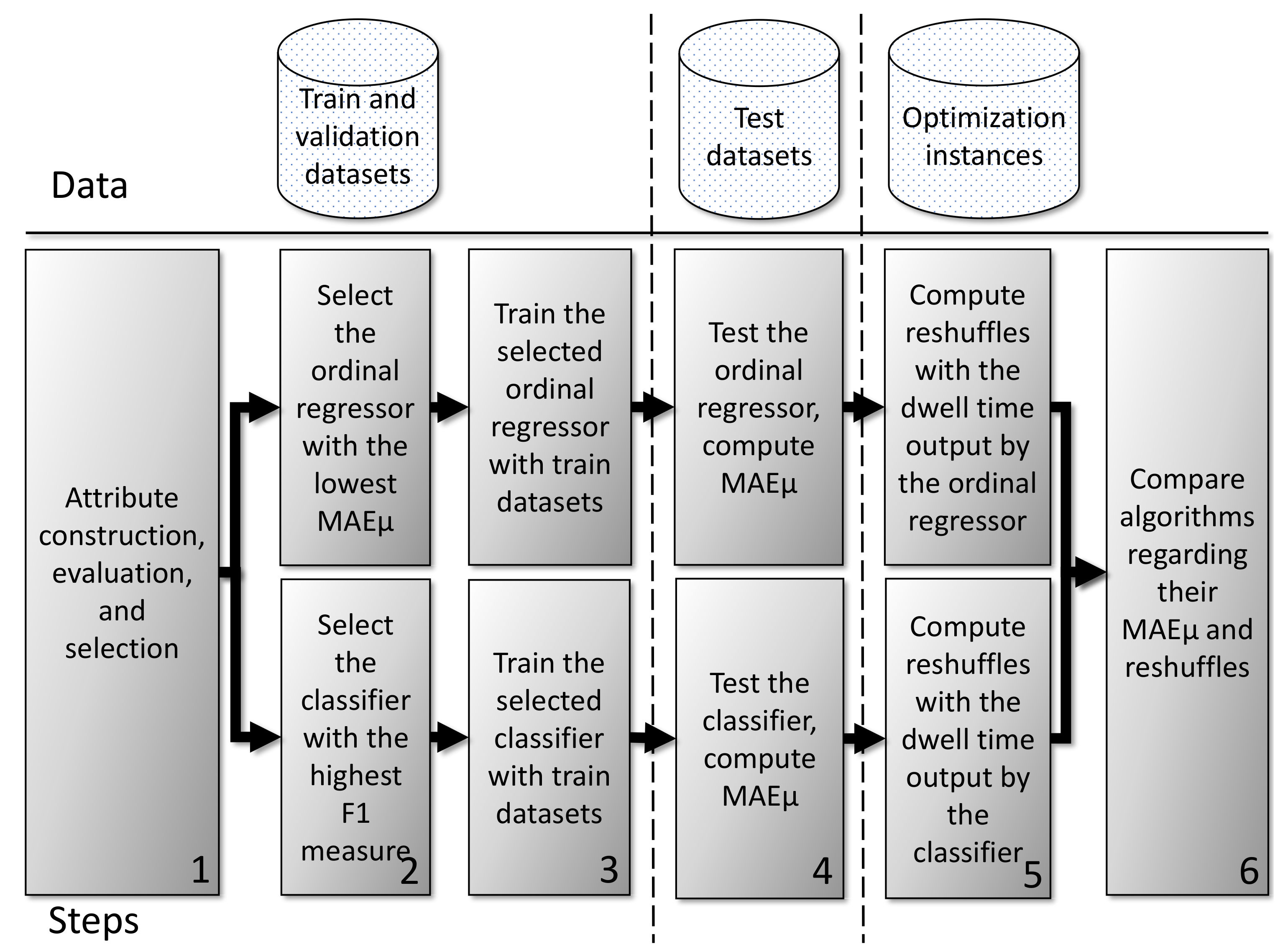
The diagram in Figure 1 describes the method followed in our experiments. We present six steps and three data sources. In step 1, we propose, evaluate, and select a set of 35 attributes using two train and validation datasets. Such a set of attributes is one of our contributions. In step 2, we train, validate, and select the algorithm for ordinal regression with the lowest $MAE\mu$ and the classifier with the highest F1 measure [31], performing cross-validation tests with ten folds. In step 3, we train the selected algorithms with the entire training data. Following, we test such algorithms in step 4, computing their $MAE\mu$ using two testing datasets. In step 5, we estimate the dwell time for containers in the testing datasets. Next, we determine the storage space for each container using the estimated dwell time. Following, we compute the reshuffles by replacing the estimated dwell time with their actual dwell time. Finally, we compare the ordinal regression approach against the classification approach regarding their $MAE\mu$ and reshuffles in step 6.

3.1. Attribute Extraction, Construction, Evaluation, and Selection

Table 2. Thirty-five attributes studied for estimating the dwell time of import containers in a yard. The second column lists the information stored by the attributes. Attributes one to four store information captured in the records of the container yard as is. The other attributes combine information captured in the records and external information.

#	Information Used as Source of the Attribute	Attribute	Domain	Type
1	Type	Type	$\left\{20,40\right\}$	Nominal
2	Client	Client	Categorical	Nominal
3	Destination	Destination	Categorical	Nominal
4	Products	Product	Categorical	Nominal
5	Date of the arrival to the country	Days_in_country	$x\in {\mathbb{Z}}^{*}$	Numeric
	Date of the arrival to the yard
6	Date of the arrival to the yard	Arrival_week_day	$s\in \mathbb{Z},1\le s\le 7$	Nominal
7		Arrival_month_day	$d\in \mathbb{Z},1\le d\le 31$	Nominal
8		Arrival_month	$m\in \mathbb{Z},1\le m\le 12$	Nominal
9	Destination	Distance_yard_destination	$k\in {\mathbb{R}}^{*}$	Numeric
10–21	Date of the arrival to the yard	Yard_weather	Categorical	Nominal
	Weather forecast
22–33	Destination	Destination_weather	Categorical	Nominal
	Date of the arrival to the yard
	Weather forecast
34	From all above attributes	Cluster	$c\in \mathbb{Z},0\le c\le 10$	Nominal
35	Date of the arrival to the yard	Predicted_dwell_time $\left(\tau \right)$	$\tau \in {\mathbb{Z}}^{*}$	Numeric
	Cluster

describes the attributes that we have extracted and constructed for estimating the dwell time.

Rows from one to four list four nominal attributes extracted directly from historical data collected by the operators of the yard: “Client”, “Destination”, “Product” (first dataset only), and “Type”, which represents the dimension of a container, i.e., 20 or 40 feet.

The other rows list attributes built from other attributes and historical data. We have constructed the attribute “Days_in_country” with the difference between the arrival date to the yard minus the arrival date to the country. Additionally, we have split the arrival date of the container to the yard into three attributes “Arrival_week_day”, “Arrival_month_day”, and “Arrival_month”. We have used the attribute “Destination” to compute the attribute “Distance_yard_destination”. Attributes “Yard_weather” and “Destination_weather” were built from the arrival date to the yard and the destination of a container. Ninety-five percent of the containers in the datasets stood in the yard for less than 12 days. Therefore, we have analyzed the weather forecast in the yard and the destination from the arrival day (0) to the day number 11 of the container in the yard. We employed the weather forecast provided by Raspisaniye Pogodi Ltd., St. Petersburg, Russia (https://rp5.ru (accessed on 25 November 2018)). This online weather-forecast service provides an overview of the weather forecast or report (for previous dates). The values for the weather overview considered were normal, light rain, heavy rain, rain, rain showers, thunderstorm, mist, precipitation within sight, fog, haze, or in the vicinity showers.

A rough estimation of the dwell time for import containers can be computed with the formula for computing the CPU burst time (see Equation (1)) [32]. This formula estimates the execution time of a task $\left({\tau }_{i+1}\right)$ using the actual $\left(t_i\right)$ and predicted $\left({\tau }_i\right)$ execution time of the previous task, weighted by $0\le \alpha \le 1$. The formula for computing the CPU burst time considers that continuous tasks have similar execution times. Sometimes, containers arrive at the yard as clusters, sharing the same client, destination, and content. This estimation is insufficient for stacking the containers because it disregards several attributes that affect the departure date. Nevertheless, we have explored the relevance of having an attribute called “Predicted_dwell_time” $\left(\tau \right)$ computed with the CPU burst time formula [32]. To compute each $\left({\tau }_i\right)$, we must group similar containers because the CPU burst time formula assumes that CPU tasks are similar. Thus, we have included another attribute called “Cluster” computed with the algorithm KMeans and the validation index VIC [33]. We have sorted containers into each cluster according to their arrival date to the country. Then, we have computed each ${\tau }_i$ for similar containers.

$${\tau }_{i+1}=\alpha t_i+\left(1-\alpha \right){\tau }_i$$

(1)

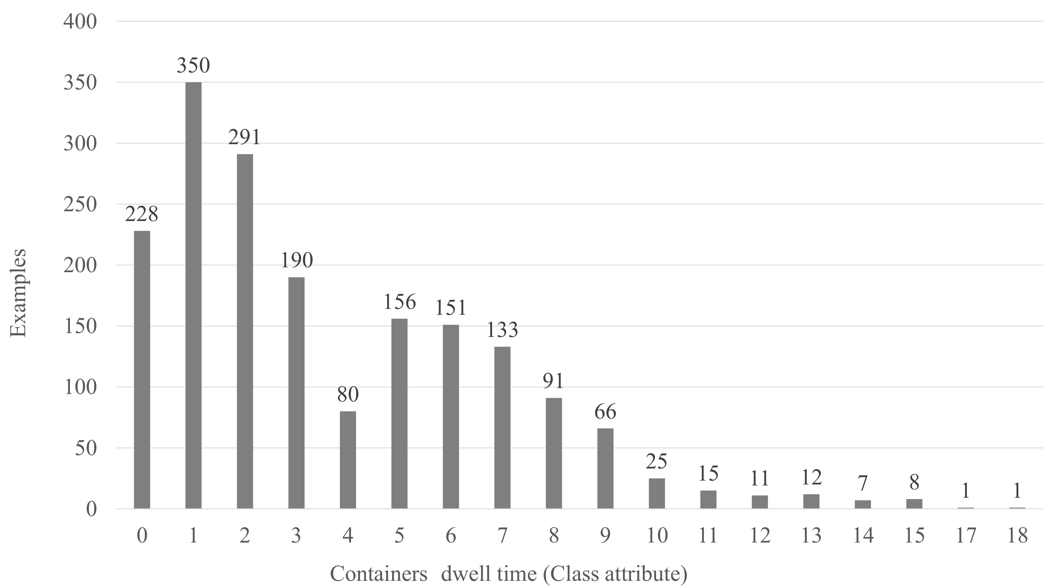
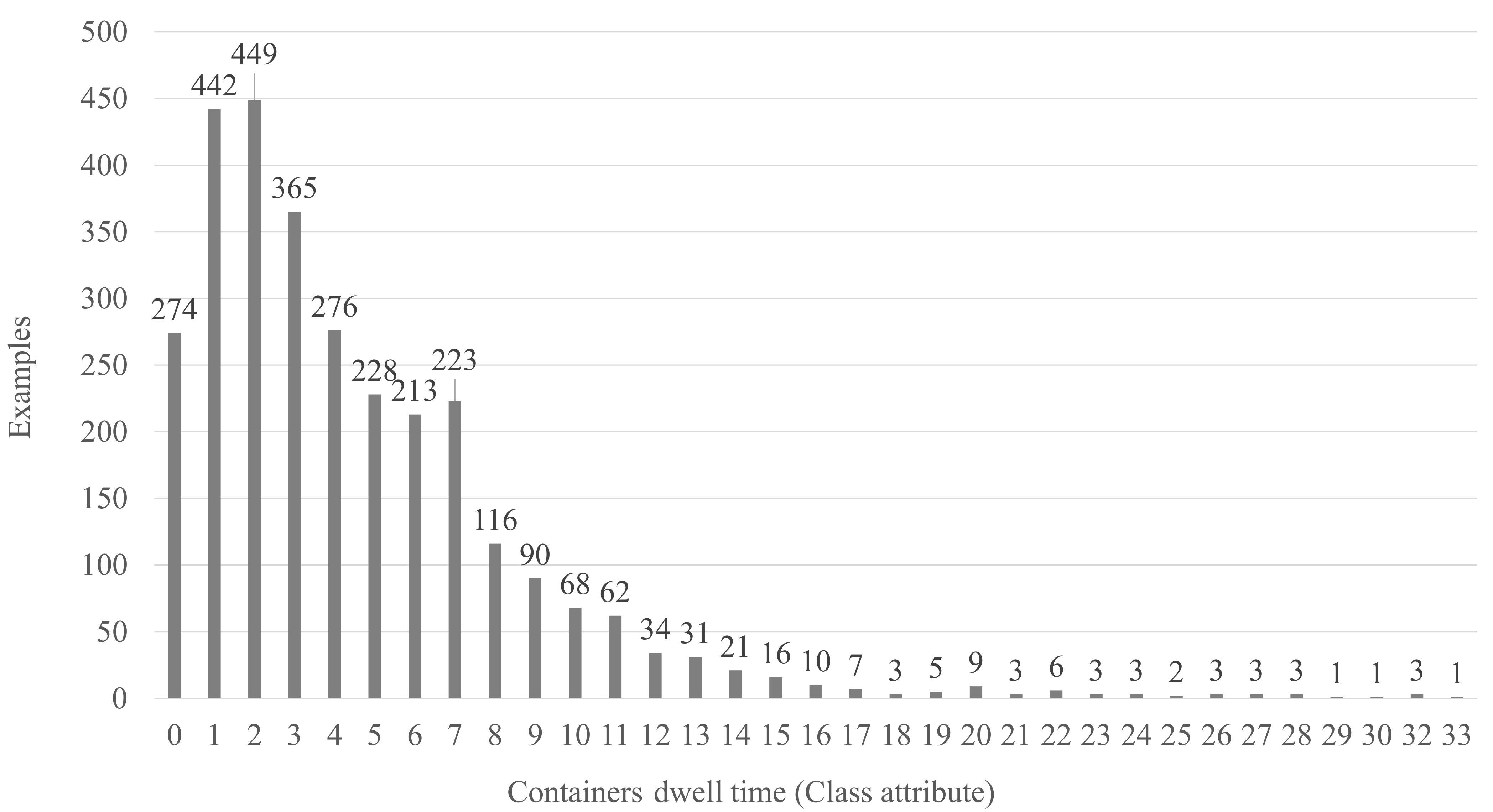
The class attribute in our datasets is “Dwell_time”. Such class attribute represents the number of days that a container stays in the yard, i.e., the number of days between the arrival and departure dates. Thus, the inferred dwell time of a container in the yard allows us to approximate its departure date and reduce the reshuffles during the unloading operations. Histograms in Figure 2 and Figure 3 plot the distribution of the actual dwell time of the containers in our datasets. These histograms depict a class imbalance in our datasets. According to a standard measure of the class imbalance [34], we have measured the imbalance ratio in $\frac{1}{350}$ and $\frac{1}{449}$, respectively. Consequently, we have employed algorithms and evaluation metrics suitable for datasets with class imbalance.

Attribute Evaluation and Selection

We have evaluated the proposed attributes based on two criteria, the correlation between each attribute and the class attribute “Dwell_time” and the correlation among all the attributes [35], and the information gain $\left(G\right)$ of each attribute concerning the “Dwell_time” (see Equation (2)). Such an information gain is based on entropy $\left(H\right)$ (see Equation (3)). We have employed the implementations in the platform WEKA version 3.8.3.

$$G(Dwell\_time,at{t}_i)=H(Dwell\_time)-H(Dwell\_time|at{t}_i)$$

(2)

$$H(Dwell\_time)=-\sum _{x\in Dwell\_time}\left(p\left(x\right)lo{g}_{2}p\left(x\right)\right)$$

(3)

With this experimental configuration and using the Dataset1_T&V, we have obtained as relevant attributes “Days _in_country”, “Arrival_week_day”, “Arrival_month_ day”, “Destination”, “Product”, and “Predicted_dwell_time”. Similarly, but using the Dataset2_T&V, we obtained as relevant attributes “Arrival_week_day”, “Destination”, and “Predicted_dwell_time”. We emphasize that the attribute “Product” is excluded in this dataset. As a result, we have selected a subset of attributes with “Days_in_country”, “Arrival_week_day”, “Arrival_month_day”, “Destination”, “Product” (first dataset only), and “Predicted_dwell_time”.

A brief analysis of the selected attributes sheds light on their worth for estimating the dwell time, justifying the results of the evaluation algorithms. For example, containers with food (attribute “Product”) remain three days on average in the yard, while containers with clothes and electronic devices remain five and eight days on average, respectively. Usually, containers have a leasing contract. Therefore, operators tend to deliver containers with several days in the country (attribute “Days_in_country”) soon, which reduces their dwell time. According to our data, most containers arriving on Monday (attribute “Arrival_week_day”) remain one day in the yard, whereas most of those arriving on Friday stay four days. Containers arriving at the beginning of the month (attribute Arrival_month_day) have lower dwell times than those arriving at the ending of the month. Moreover, the data show that containers with a destination (attribute “Destination”) near the yard are delivered faster than those with far destinations. Although we built an attribute with the distance from the yard to the destination of a container, the attribute “Destination” reached a higher evaluation than this distance. The attribute “Predicted_dwell_time” is relevant because of the similarities between some arrival containers, such as tasks in a CPU planner.

3.2. Dwell Time Estimation as an Ordinal Regression Problem

To determine the best performed ordinal regression algorithm, we have evaluated 15 algorithms proposed in the literature. These algorithms follow three approaches: a naive approach, an ordinal learning approach, and an approach based on decomposing ordinal problems into binary problems. We employed the implementations in the platform WEKA version 3.8.3.

An ordinal regression algorithm with a naive approach consists of converting the values of the ordinal class attribute into numerical values, “Dwell_time” in our case. Next, a naive approach applies a regression algorithm $\left(\delta \right)$ and uses one of the rounding strategies to map the continuous value calculated by the regressor $\left(\delta \right)$ to an ordinal value of the original class (see Equation (4)).

$$Dwell\_time\left(att\right)=\left\{\begin{array}{cc}\lfloor \delta \left(att\right)\rfloor \hfill & floor\hfill \\ \lfloor \delta \left(att\right)\rceil \hfill & round\hfill \\ \lceil \delta \left(att\right)\rceil \hfill & ceiling\hfill \end{array}\right.$$

(4)

We have explored five algorithms with this approach:

• Regression using DecisionTable, and optimizing root mean square error
  (Reg + DecisionTable + RMSE + Ibk + Round)
• Regression using LibSVM with linear kernel and rounding
  (Reg + LibSVM + LinearKernel + Round)
• Linear regression with rounding (Reg + LinearRegression + Round)
• Classification via regression using a Linear regression (CvR + LinearRegression)
• Classification via regression using the algorithm M5P (CvR + M5P)

The second approach is called the Ordinal Learning Method (OLM) [36]. OLM generates symbolic rules using comparison operations from examples in ordinal problems with multiple attributes. The algorithm to generate the symbolic classification rules aims to simulate human behavior when solving ordinal regression problems. The author of OLM tested the performance of the algorithm OLM on four datasets achieving results similar to the decision tree C4 for ordinal regression problems.

The third approach is based on decomposing ordinal problems into binary problems with the OrdinalClassClassifier (OCC) [37] method. The algorithm OCC uses supervised classifier for solving problems with ordinal classes. For such a purpose, the algorithm OCC creates a new dataset for each value $(\Vert Dwell\_time\Vert )$ of the ordinal class attribute. New datasets have a new binary class attribute instead of the ordinal class. Such a binary class takes value 1 for the examples for which the ordinal class had a value greater than the index of the current dataset. Then, a supervised classifier is trained with the modified datasets obtaining a model for each dataset. To classify a new example $\left(att\right)$, each model classifies the example and computes the likelihood of belonging to the binary class $\left(p_i\left(att\right)\right)$. With these likelihoods, the algorithm OCC computes new values according to the index of the model trained. In the last step, the algorithm OCC selects the class value in the ordinal class attribute corresponding to the index of the max new value computed (see Equation (5)).

$$Dwell\_time\left(att\right)=\underset{i\in \Vert Dwell\_time\Vert }{argmax}\left\{\begin{array}{cc}1-p_i\left(att\right),\hfill & i=1\hfill \\ p_{i-1}\left(att\right)-p_i\left(att\right),\hfill & 1<i<\Vert Dwell\_time\Vert \hfill \\ p_i\left(att\right),\hfill & i=\Vert Dwell\_time\Vert \hfill \end{array}\right.$$

(5)

We have explored the combination of the method OCC with the classifiers listed below. We have included four kernels (linear, polynomial, RBF, and sigmoidal) for the classifier Support Vector Machine (SVM).

• OCC + IBk1
• OCC + Kernel Logistic Regression
• OCC + LibSVM + LinearKernel
• OCC + LibSVM + PolyKernel
• OCC + LibSVM + RBFKernel
• OCC + LibSVM + SigmoidKernel
• OCC + C4.5
• OCC + MLP − RELU
• OCC + SimpleLogistic

A conventional metric to evaluate the performance of ordinal regression methods is Mean Absolute Error (MAE) [38,39,40,41,42,43,44]. This metric measures the magnitude of the error of each ordinal algorithm, e.g., a 4-days error in the prediction of a container’s dwell time is higher than a 1-day error. However, MAE biases the results favoring the majoritarian class when the dataset shows a class imbalance. Our datasets present class imbalance (see Figure 2 and Figure 3). Therefore, we have adopted the Mean Absolute Error modified ($MAE\mu$) [45] as the performance measure. $MAE\mu$ is a modification of MAE for imbalanced datasets that consists of computing the MAE for each value of the class attribute in the dataset and then averaging the results.

Table 3. $MAE\mu$ achieved by 15 ordinal regression algorithms with both datasets for training and validation. The Ordinal Class Classifier with a Kernel Logistic Regression achieved the lowest error ($MAE\mu$) on both datasets.

Algorithm	Dataset1_T&V	Dataset2_T&V
OCC + IBk k = 1	3.331590404	7.08567135
OCC + Kernel Logistic Regression	2.431074447	6.396608677
OCC + LibSVM + LinearKernel	3.152352826	7.64170435
OCC + LibSVM + PolyKernel	5.221540441	13.03492621
OCC + LibSVM + RBFKernel	4.982034132	12.13935106
OCC + LibSVM + SigmoidKernel	6.131968673	12.36516552
OCC + C4.5	3.703891075	9.843052078
OLM	3.085444781	8.04021403
OCC + MLP − RELU	2.643779925	8.273726134
OCC + SimpleLogistic	4.857876774	14.13145068
CvR + LinearRegression	3.251455833	8.364204478
CvR + M5P	3.745751895	8.440288676
Reg + DecisionTable + RMSE + Ibk + Round	5.558925374	12.06379664
Reg + LibSVM + LinearKernel + Round	5.788572492	12.13227507
Reg + LinearRegression + Round	5.798134705	12.13779264

summarizes the $MAE\mu$ output by the algorithms with both training datasets. The OCC algorithm with the Kernel Logistic Regression method as classifier achieved the lowest $MAE\mu$ for both datasets. Hence, we select OCC + Kernel Logistic Regression to estimate the dwell time.

3.3. Dwell Time Estimation as a Supervised Classification Problem

To determine the supervised classification algorithms, we have used the Auto-WEKA tool [46] included in WEKA version 3.8.3. Auto-WEKA compares the performance of 30 supervised learning algorithms regarding a metric selected by the user using a cross-validation test with ten folds. Since our datasets present a class imbalance in a ratio of $\frac{1}{350}$ and $\frac{1}{449}$, respectively, we configured Auto-WEKA to select the classification algorithm with the highest F1 measure.

Auto-WEKA outputs a different supervised classifier for each dataset. The algorithm with the highest F1 measure -0.91- estimating the dwell time for the instances in the Dataset1_T&V was Lazy-IBK with the parameters [−E, −K, 29, −X, −I]. However, Lazy-KStar with the parameters [−B, 4, −M, a] reached the highest F1 measure -0.90- estimating the dwell time for the instances in the Dataset2_T&V.

Previously, we found that the algorithm OCC with Kernel Logistic Regression reached the lowest $MAE\mu$ for both datasets by estimating the dwell time as an ordinal regression problem. To achieve this result, we performed several experiments manually configured. Contrarily, Auto-WEKA found a different supervised classifier for each dataset. However, since we aim to show that estimating the dwell time for import containers in a yard must be solved as an ordinal regression problem, we shall compare the three algorithms, OCC+Kernel Logistic Regression, against Lazy-IBK on Dataset1_Test and OCC+Kernel Logistic Regression against Lazy-KStar on Dataset2_Test.

4. Results and Discussion

We have assumed that by estimating the dwell time with an ordinal regression algorithm, we can reduce the reshuffles in the container stacking compared to those produced with supervised classification algorithms. The ordinal regression algorithm OCC + Kernel Logistic Regression reached the lowest MAE$\mu$ in our previous experiments with 15 ordinal regression algorithms using the two training and validation datasets (Dataset1_T&V and Dataset2_T&V). However, we have selected two supervised classifiers (Lazy-IBK and Lazy-KStar) for each dataset according to the results of the Auto-WEKA tool.

There is no consensus about the measures to evaluate the worthiness of the estimated dwell time with machine-learning algorithms for the optimal stacking of containers. Since we have estimated the dwell time as an ordinal regression problem, we can employ the $MAE\mu$ as a practical measure. We can also compute the $MAE\mu$ for estimating the dwell time as a supervised classification problem but considering the size of the error. Thus, we can compare the performance of both approaches. Moreover, we have included the number of reshuffles as another performance measure, starting from the estimated departure date of each container computed with the date of the arrival to the yard and the estimated dwell time. Using the estimated departure date, we have allocated the containers with the optimization model proposed by De Armas et al. [2] and implemented using the solver GNU Linear Programming Kit (GLPK (http://www.gnu.org/software/glpk (accessed on 14 July 2019))) version 4.64. The optimization algorithm output a matrix with the positions assigned to the containers in the yard. Finally, we have substituted the estimated departure date of each container with its actual departure date (obtained from the recorded data) and computed the number of reshuffles.

We have considered three configurations of the container yard (45 stacks with three tiers, 90 stacks with three tiers, and 45 stacks with five tiers). We have started with an empty yard for each configuration, with the maximum number of allocation spaces available. Moreover, we have set up 21 optimization instances (see

Table 4. Description of the optimization instances regarding the dataset and the number of examples, stacks, tiers, and slots.

Optimization Instance ID	Dataset	Examples	Stacks	Tiers	Slots
1, 2, 3	Dataset1_Test	135	45	3	135
4		49
5, 6, 7, 8, 9	Dataset2_Test	135
10		68
11, 12	Dataset1_Test	227	90	3	270
13, 14	Dataset2_Test	248
15		247
16, 17	Dataset1_Test	225	45	5	225
18, 19, 20	Dataset2_Test
21		68

) using the examples in the datasets Dataset1_Test and Dataset2_Test.

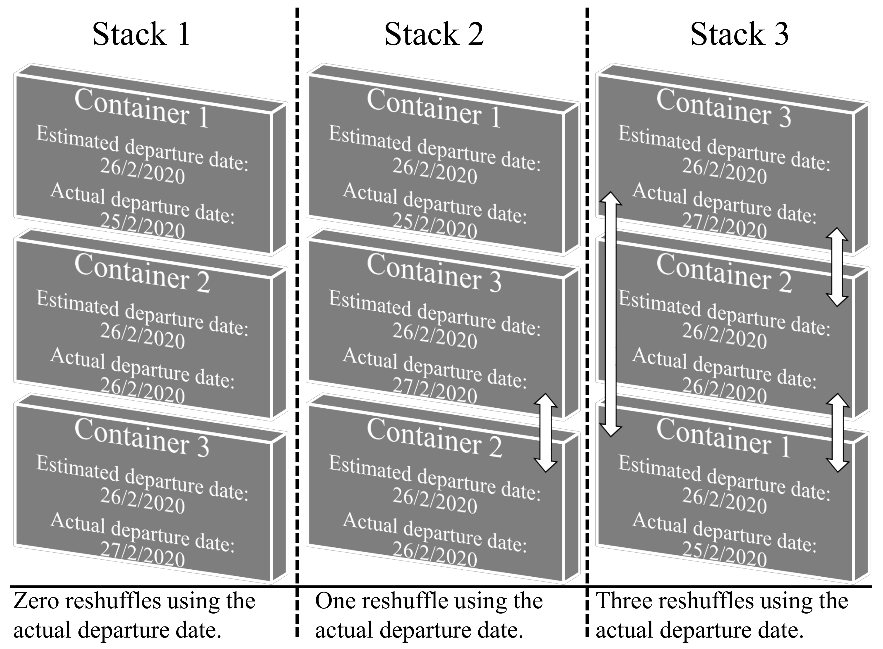
An optimization algorithm can reach the optimal solution with different containers’ allocations. Therefore, such an optimization algorithm can yield dissimilar numbers of reshuffles for the same optimization instance. Reshuffles come from the use of the estimated departure date for optimizing the containers’ allocation but the actual departure date for computing the reshuffles. Figure 4 illustrates an example with three allocations to the containers with the same optimization value (0 reshuffles) but different numbers of actual reshuffles. Therefore, reducing the $MAE\mu$ does not always reduce the number of reshuffles, but in general, it does, as we shall show with our experimental results.

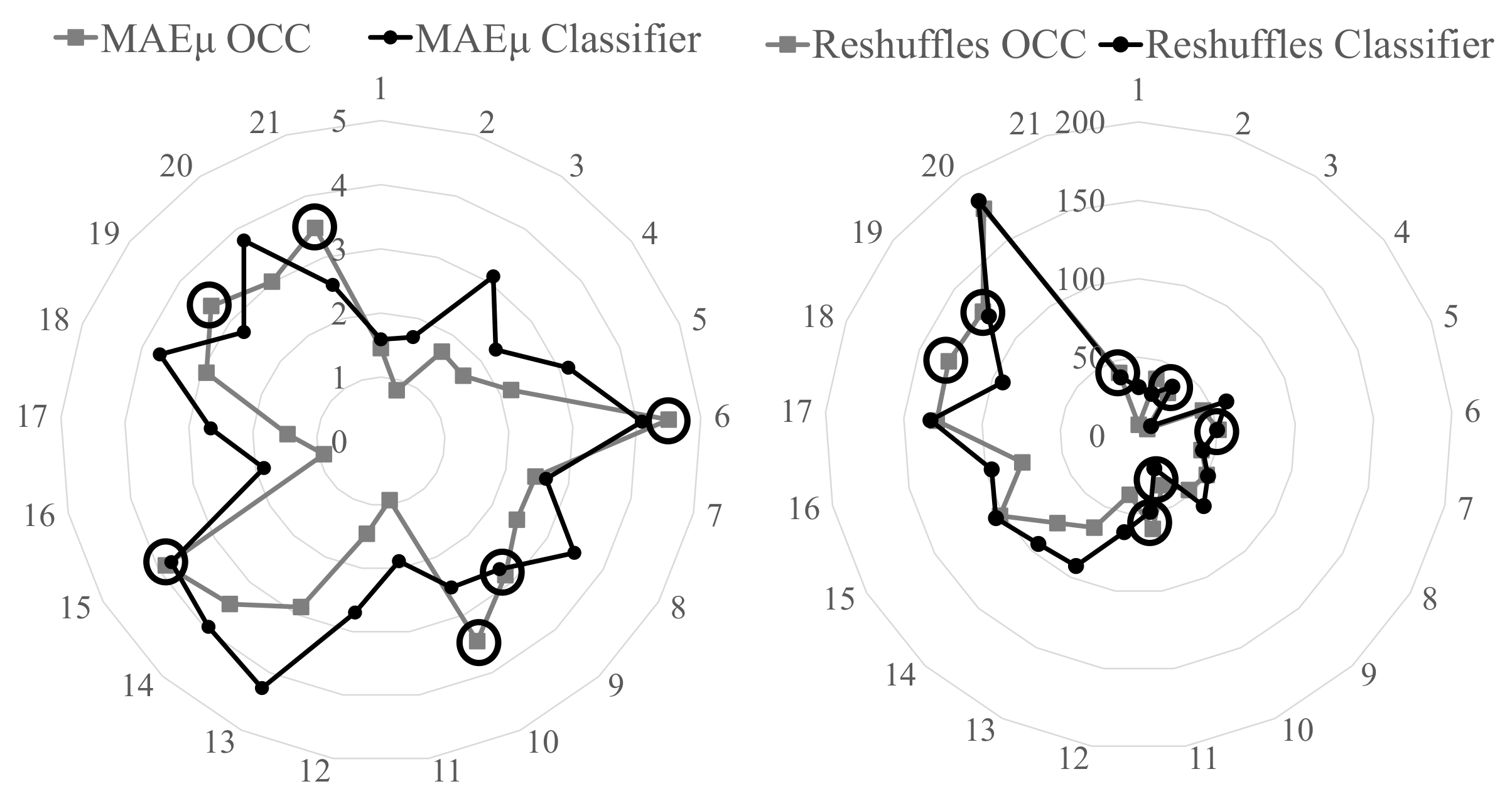
Figure 5 depicts the $MAE\mu$ (left) obtained by the ordinal regression algorithm and the respective supervised classification algorithm for each optimization instance. Moreover, the figure depicts the number of reshuffles (right) computed by the optimization algorithm using those departure dates estimated with the ordinal regression algorithm and the respective supervised classification algorithm. Black circles indicate those instances where the ordinal regression algorithm lost against the respective supervised classification algorithm.

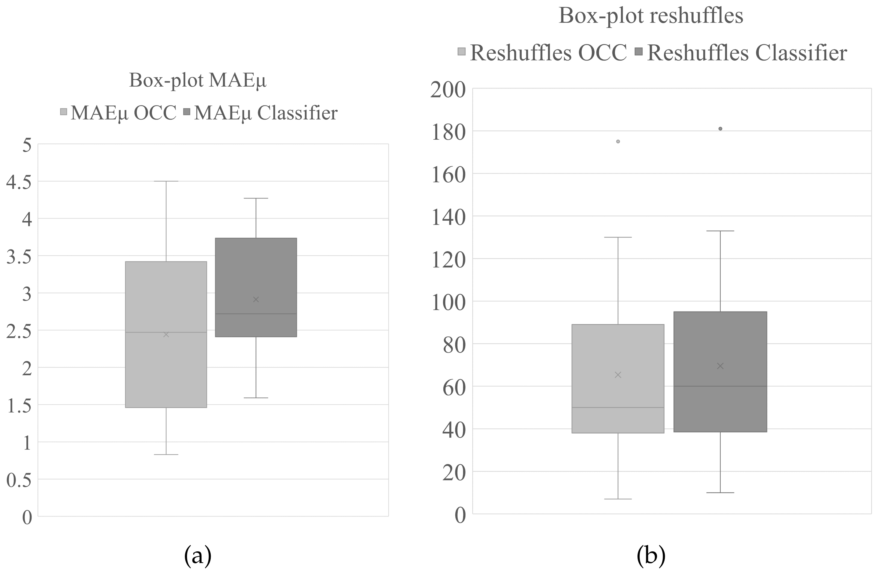
Figure 6 illustrates box plots for both methods, ordinal regression and classification. Both graphs ($MAE\mu$ and reshuffles) show lower median errors for the ordinal regression approach. The classification method shows lower dispersion in the $MAE\mu$ than the ordinal regression method, while the ordinal regression method shows the lower quartile values. Likewise, the ordinal regression yielded lower second and third quartiles than the classification method regarding the reshuffles, but the min, max, and first quartile values were similar. These distributions indicate differences between the methods higher concerning the $MAE\mu$ than the reshuffles because of the effect of the optimization algorithm.

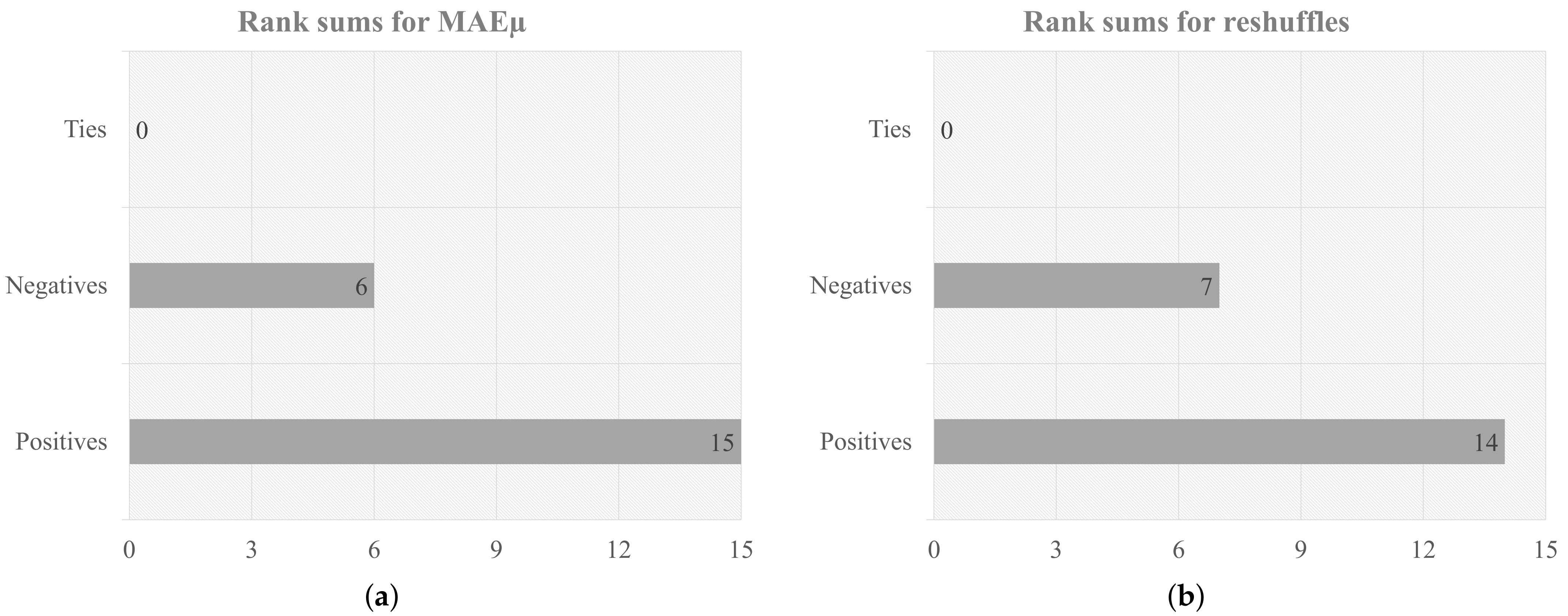
The ordinal regression algorithm reached a lower $MAE\mu$ for 15 ($71\%$) instances and a lower number of reshuffles for 14 ($67\%$) instances. Figure 7 depicts the rank sums comparing the ordinal regression against the classification regarding $MAE\mu$ and reshuffles. The Wilcoxon signed ranks test [47] indicated that there were significant differences between both methods regarding the $MAE\mu$ (p-value = 0.009128), but the differences were not significant regarding the reshuffles (p-value = 0.1393). Nevertheless, the dwell time estimated with the ordinal regression algorithm generated 87 reshuffles less than the estimated with the supervised classifiers in these 21 experiments. Additionally, in 16 of these experiments, a lower $MAE\mu$ induced a lower number of reshuffles. The other five experiments showed a different behavior due to the influence of the optimization algorithm previously explained.

From these results, we conclude that the dwell time of the containers is estimated more accurately as an ordinal regression problem than as a supervised classification problem, at least using these attributes of the containers. Moreover, all the algorithms reached a higher $MAE\mu$ and number of reshuffles using the examples in the Dataset2_Test than the examples in Dataset1_Test (instances 1, 2, 3, 4, 11, 12, 16, and 17). Since only Dataset1 includes the attribute “Product”, we recommend including this attribute to improve the algorithms for the dwell time estimation.

5. Conclusions

In this work, we aimed to show that estimating the dwell time of import containers in a yard is an ordinal regression problem. Thus, we modeled and solved the problem as both an ordinal regression problem and a supervised classification problem; this last is the trending approach in the literature. To corroborate our hypothesis, we compute the $MAE\mu$, and the reshuffles provoked during the container stacking using the dwell time estimated by each approach.

As a result of our research, we noticed that the ordinal regression algorithm achieved the lowest $MAE\mu$ in 15 ($71\%$) of our 21 experiments. Similarly, the ordinal regression algorithm yielded the lowest reshuffles in 14 ($67\%$) experiments. The statistical test corroborated significant differences between both methods regarding the $MAE\mu$, while differences were not significant regarding the reshuffles. Since different optimal allocations of the containers can lead to different numbers of reshuffles, we examined the relationship between $MAE\mu$ and reshuffles. We noticed that a lower $MAE\mu$ conducts to a lower number of reshuffles in 16 ($76\%$) experiments. Therefore, we can state that by modeling the dwell time estimation as an ordinal regression problem and decreasing the $MAE\mu$, we can reduce the number of reshuffles generated during the stacking of import containers in a yard.

We found a subset of six attributes relevant for estimating the dwell time of import containers in a terminal from a set of 35 evaluated. Such attributes are “Days _in_country”, “Arrival_week_day”, “Arrival_month_day”, “Destination”, “Product”, and “Predicted_dwell _time”. The attribute “Predicted_dwell _time” approximates the dwell time using the formula to compute the CPU burst time in groups of similar containers. Attributes “Days _in_country”, “Arrival_week_day”, “Arrival_month_day” are derived from the arrival date of the containers to the country. “Destination” and “Product” were obtained from the containers’ information. Moreover, we evaluated 25 attributes related to the weather forecast and the distance between the yard and the destination of the container. Such an evaluation showed that they were irrelevant for the dwell time estimation of the containers in our datasets.

We observed that all the algorithms produced a higher $MAE\mu$ and reshuffles for the examples in the dataset that excluded the attribute “Product”. Hence, we recommend including the attribute “Product” for estimating the dwell time of import containers in a yard. Nevertheless, further experiments are needed to support this recommendation.

Our results can be applied on dwell time estimation problems where the dwell time is an ordinal variable. Two additional examples of these problems are the dwell time estimation of ships in docks and the dwell time of buses in a bus workshop for repairing. For these examples, an accurate dwell time estimation may conduct to saving resources, as our research work does.

We propose evaluating other ordinal regression algorithms, such as deep neural networks for ordinal regression, as future work. Moreover, we shall be working on a new dataset about import containers available for the research community to reduce the lack of available datasets.

References

- Yu, M.; Liang, Z.; Teng, Y.; Zhang, Z.; Cong, X. The inbound container space allocation in the automated container terminals. Expert Syst. Appl. 2021, 179, 115014. [Google Scholar] [CrossRef]
- De Armas Jacomino, L.; Valdes-Ramirez, D.; Morell Pérez, C.; Bello, R. Solutions to Storage Spaces Allocation Problem for Import Containers by Exact and Heuristic Methods. Comput. Sist. 2019, 23, 197–211. [Google Scholar]
- Zhou, L.; Sun, L.; Li, Z.; Li, W.; Cao, N.; Higgs, R. Study on a storage location strategy based on clustering and association algorithms. Soft Comput. 2020, 24, 5499–5516. [Google Scholar] [CrossRef] [Green Version]
- Lee, I.G.; Chung, S.H.; Yoon, S.W. Two-stage storage assignment to minimize travel time and congestion for warehouse order picking operations. Comput. Ind. Eng. 2020, 139, 106–129. [Google Scholar] [CrossRef]
- Lersteau, C.; Nguyen, T.T.; Le, T.T.; Nguyen, H.N.; Shen, W. Solving the Problem of Stacking Goods: Mathematical Model, Heuristics and a Case Study in Container Stacking in Ports. IEEE Access 2021, 9, 25330–25343. [Google Scholar] [CrossRef]
- Zhen, L.; Jiang, X.; Hay Lee, L.; Chew, E.P. A Review on Yard Management in Container Terminals. Ind. Eng. Manag. Syst. 2013, 12, 289–305. [Google Scholar] [CrossRef]
- Maldonado, S.; González-Ramírez, R.G.; Quijada, F.; Ramírez-Nafarrate, A. Analytics meets port logistics: A decision support system for container stacking operations. Decis. Support Syst. 2019, 121, 84–93. [Google Scholar] [CrossRef]
- Kim, K.H.; Yi, S. Utilizing information sources to reduce relocation of inbound containers. Marit. Econ. Logist. 2021. [Google Scholar] [CrossRef]
- Kourounioti, I.; Polydoropoulou, A.; Tsiklidis, C. Development of models predicting dwell time of import containers in port container terminals an Artificial Neural Networks application. Transp. Res. Procedia 2016, 14, 243–252. [Google Scholar] [CrossRef] [Green Version]
- Zhou, S.F.; Zhang, Q.N. Model of Mining the Synchronism of Retrieval Processes Between Customers for Optimizing the Import Container Allocation Problem. In Proceedings of the International Conference on Management Science and Industrial Engineering, Phuket, Thailand, 24–26 May 2019; ACM: New York, NY, USA, 2019; pp. 117–125. [Google Scholar]
- Zhu, H.; Ji, M.; Guo, W. Two-stage search algorithm for the inbound container unloading and stacking problem. Appl. Math. Model. 2020, 77, 1000–1024. [Google Scholar] [CrossRef]
- Yan, B.; Zhu, X.; Lee, D.H.; Jin, J.G.; Wang, L. Transshipment operations optimization of sea-rail intermodal container in seaport rail terminals. Comput. Ind. Eng. 2020, 141, 106296. [Google Scholar] [CrossRef]
- Boge, S.; Knust, S. The parallel stack loading problem minimizing the number of reshuffles in the retrieval stage. Eur. J. Oper. Res. 2020, 280, 940–952. [Google Scholar] [CrossRef]
- Nadereh, M.; Maria, B.; Sotiris, T.; William, L. Estimating the determinant factors of container dwell times at seaports. Marit. Econ. Logist. 2012, 14, 162–177. [Google Scholar]
- Rodriguez-Molins, M.; Salido, M.A.; Barber, F. Intelligent planning for allocating containers in maritime terminals. Expert Syst. Appl. 2012, 39, 978–989. [Google Scholar] [CrossRef] [Green Version]
- Gaete, M.; González-Araya, M.C.; González-Ramírez, R.G.; Astudillo, C. A Dwell Time-based Container Positioning Decision Support System at a Port Terminal. In Proceedings of the 6th International Conference on Operations Research and Enterprise Systems (ICORES), Porto, Portugal, 23–25 February 2017; SciTePress: Setúbal, Portugal, 2017. [Google Scholar]
- Kourounioti, I.; Polydoropoulou, A. Identification of Container Dwell Time Determinants Using Aggregate Data. Int. J. Transp. Econ. 2017, 44, 567–588. [Google Scholar]
- Oh, Y.; Byon, Y.J.; Song, J.Y.; Kwak, H.C.; Kang, S. Dwell Time Estimation Using Real-Time Train Operation and Smart Card-Based Passenger Data: A Case Study in Seoul, South Korea. Appl. Sci. 2020, 10, 476. [Google Scholar] [CrossRef] [Green Version]
- Luo, J.; Wu, Y.; Halldorsson, A.; Song, X. Storage and stacking logistics problems in container terminals. OR Insight 2011, 24, 256–275. [Google Scholar] [CrossRef]
- Gaete, M.; González-Araya, M.C.; González-Ramírez, R.G.; Astudillo, C. A Novel Storage Space Allocation Policy for Import Containers. In Proceedings of the International Conference on Operations Research and Enterprise Systems, Porto, Portugal, 23–25 February 2017; Springer: Berlin/Heidelberg, Germany, 2017; pp. 293–316. [Google Scholar]
- Zhu, H.; Shan, H.; Zhang, Y.; Che, L.; Xu, X.; Zhang, J.; Shi, J.; Wang, F.Y. Convolutional ordinal regression forest for image ordinal estimation. IEEE Trans. Neural Netw. Learn. Syst. 2021, 1–12. [Google Scholar] [CrossRef]
- Yong, C.W.; Teo, K.; Murphy, B.P.; Hum, Y.C.; Tee, Y.K.; Xia, K.; Lai, K.W. Knee osteoarthritis severity classification with ordinal regression module. Multimed. Tools Appl. 2021, 1–13. [Google Scholar] [CrossRef]
- Ci, T.; Zhen, L.; Wang, Y. Assessment of the degree of building damage caused by disaster using convolutional neural networks in combination with ordinal regression. Remote Sens. 2019, 11, 2858. [Google Scholar] [CrossRef] [Green Version]
- Nennuri, R.; Yadav, M.G.; Vahini, Y.S.; Prabhas, G.S.; Rajashree, V. Twitter Sentimental Analysis based on Ordinal Regression. J. Phys. Conf. Ser. 2021, 1979, 012069. [Google Scholar] [CrossRef]
- Winship, C.; Mare, R.D. Regression models with ordinal variables. Am. Sociol. Rev. 1984, 49, 512–525. [Google Scholar] [CrossRef]
- Niu, Z.; Zhou, M.; Wang, L.; Xinbo, G.; Hua, G. Ordinal regressionwith multiple output CNN for age estimation. In Proceedings of the IEEE Conference on Computer Vision and Pattern Recognition CVPR, Las Vegas, NV, USA, 27–30 June 2016; pp. 4920–4928. [Google Scholar]
- Berg, A.; Oskarsson, M.; Mark, O. Deep ordinal regression with label diversity. In Proceedings of the 25th International Conference on Pattern Recognition (ICPR), Milan, Italy, 10–15 January 2021; pp. 2740–2747. [Google Scholar]
- Fu, H.; Gong, M.; Wang, C.; Kayhan, B.; Tao, D. Deep Ordinal Regression Network for Monocular Depth Estimation. In Proceedings of the IEEE Conference on Computer Vision and Pattern Recognition CVPR, Salt Lake City, UT, USA, 18–23 June 2018; pp. 2002–2011. [Google Scholar]
- Carlo, H.J.; Vis, I.F.; Jan Roodbergen, K. Storage yard operations in container terminals: Literature overview, trends, and research directions. Eur. J. Oper. Res. 2014, 235, 412–430. [Google Scholar] [CrossRef]
- Lehnfeld, J.; Knust, S. Loading, unloading and premarshalling of stacks in storage areas: Survey and classification. Eur. J. Oper. Res. 2014, 239, 297–312. [Google Scholar] [CrossRef]
- Lewis, D.; Gale, W. Training text classifiers by uncertainty sampling. In Proceedings of the 17th Annual International SIGIR Conference on Research and Development in Information Retrieval, Dublin, Ireland, 3–6 July 1994; ACM: New York, NY, USA, 1994; pp. 3–12. [Google Scholar]
- Silberschatz, A.; James Lyle, P.; Peter, B.G. Operating System Concepts, 9th ed.; Addison-Wesley: Boston, MA, USA, 1988. [Google Scholar]
- Rodríguez, J.; Medina-Pérez, M.A.; Gutierrez-Rodríguez, A.E.; Monroy, R.; Terashima-Marín, H. Cluster validation using an ensemble of supervised classifiers. Knowl.-Based Syst. 2018, 145, 134–144. [Google Scholar] [CrossRef]
- Loyola-González, O.; Martínez-Trinidad, J.F.; Carrasco-Ochoa, J.A.; García-Borroto, M. Effect of class imbalance on quality measures for contrast patterns: An experimental study. Inf. Sci. 2016, 374, 179–192. [Google Scholar] [CrossRef]
- Hall, M.A. Correlation-Based Feature Subset Selection for Machine Learning. Ph.D. Thesis, University of Waikato, Hamilton, New Zealand, 1998. [Google Scholar]
- Ben-David, A. Automatic generation of symbolic multiattribute ordinal knowledge-based DSSs: Methodology and applications. Decis. Sci. 1992, 23, 1357–1372. [Google Scholar] [CrossRef]
- Frank, E.; Hall, M. A simple approach to ordinal classification. In Proceedings of the European Conference on Machine Learning, Freiburg, Germany, 5–7 September 2001; pp. 145–156. [Google Scholar]
- Chu, W.; Ghahramani, Z. Gaussian Processes for Ordinal Regression. J. Mach. Learn. Res. 2005, 6, 1019–1041. [Google Scholar]
- Chu, W.; Keerthi, S.S. Support Vector Ordinal Regression. Neural Comput. 2007, 19, 792–815. [Google Scholar] [CrossRef]
- Sun, B.Y.; Li, J.; Wu, D.D.; Zhang, X.M.; Li, W.B. Kernel Discriminant Learning for Ordinal Regression. IEEE Trans. Knowl. Data Eng. 2010, 22, 906–910. [Google Scholar] [CrossRef]
- Gu, B.; Shen, V.S.; Tay, K.Y.; Romano, W.; Li, S. Incremental support vector learning for ordinal regression. IEEE Trans. Neural Netw. Learn. Syst. 2014, 26, 1403–1416. [Google Scholar] [CrossRef] [PubMed]
- Gutiérrez, P.A.; Pérez-Ortiz, M.; Sánchez-Monedero, J.; Fernández-Navarro, F.; Hervás-Martínez, C. Ordinal regression methods: Survey and experimental study. IEEE Trans. Knowl. Data Eng. 2016, 28, 127–146. [Google Scholar] [CrossRef] [Green Version]
- Nguyen, B.; Morell, C.; De Baets, B. Distance metric learning for ordinal classification based on triplet constraints. Knowl.-Based Syst. 2018, 142, 17–28. [Google Scholar] [CrossRef]
- Pan, W. An Improved Feature Selection Algorithm for Fault Level Identification. In Recent Trends in Intelligent Computing, Communication and Devices; Springer: Berlin/Heidelberg, Germany, 2020; pp. 87–94. [Google Scholar]
- Baccianella, S.; Esuli, A.; Sebastiani, F. Evaluation Measures for Ordinal Regression. In Proceedings of the 9th International Conference on Intelligent Systems Design and Applications, Pisa, Italy, 30 November–2 December 2009. [Google Scholar]
- Thornton, C.; Hutter, F.; Hoos, H.H.; Leyton-Brown, K. Auto-WEKA: Combined selection and hyperparameter optimization of classification algorithms. In Proceedings of the 19th SIGKDD International Conference on Knowledge Discovery and Data Mining, Chicago, IL, USA, 11–14 August 2013; ACM: New York, NY, USA, 2013; pp. 847–855. [Google Scholar]
- Demšar, J. Statistical comparisons of classifiers over multiple data sets. J. Mach. Learn. Res. 2006, 7, 1–30. [Google Scholar]
Figure 1.
Steps and data sources used in the experiments for comparing the dwell time estimation with an ordinal regression approach against the dwell time estimation with a classification approach.
Figure 2.
Histogram of the containers’ dwell time in the full Dataset1, i.e., both Dataset1_T&V and Dataset1_Test.
Figure 3.
Histogram of the containers’ dwell time in the full Dataset2, i.e., both Dataset2_T&V and Dataset2_Test.
Figure 4.
Example of three different space allocations to the same containers. These allocations achieve the same optimization value, zero reshuffles computed using the estimated departure date, but three different numbers of reshuffles. White arrows indicate container pairs that generate reshuffles.
Figure 5.
Radial graphs with the (left) and reshuffles (right) output by each algorithm inferring the dwell time using both datasets split into 21 instances. A black circle encloses each instance where the ordinal regression algorithm lost against the supervised classification algorithm, i.e., six regarding and seven regarding the reshuffles.
Figure 6.
Box plots describing the (a) and the reshuffles (b) output by the ordinal regression and the classification methods.
Figure 7.
Bar graphs with rank sums computed with the Wilcoxon signed ranks test comparing the ordinal regression method vs. the classification method regarding (a) and reshuffles (b). Positive ranks specify a better performance for the ordinal regression method.