1. Introduction
Compared with other electromagnetic pulse (EMP) effects, the high-altitude electromagnetic pulse (HEMP) proves to be more powerful and irradiates more energy. The HEMP is a near-instantaneous electromagnetic energy field that is produced by the power and radiation of nuclear events such as the Chernobyl nuclear power plant accident [
1]. It poses the most serious threat to various electronic devices or systems on aircraft [
2,
3]. Hence, it should be given greater consideration during the protection design of the craft. Due to the wide frequency range of the HEMP, it can go through not only the antenna and transmission line, but also through holes or gaps and into the system, which leads to internal damage of electronic equipment or devices.
Many studies on the antenna or cable coupling with the EMP [
4,
5] show that airborne electronic devices or systems are increasingly sensitive to EMP interference with the miniaturization and integration of electronic devices. For airborne equipment system within a HEMP environment, a very strong pulse voltage or current is generated, which can interfere with the reception or transmission of signals from the equipment. However, the airborne equipment system may become damaged if the coupled voltage or current exceeds the threshold value [
5].
Considering the importance and vulnerability of airborne equipment, HEMP protection of airborne equipment is necessary. Therefore, it is necessary to carry out research related to HEMP protection so that airborne equipment systems can still operate reliably within a specified period in a HEMP environment. Furthermore, this research paper on HEMP protection for typical airborne frequency equipment will focus on the mechanisms and the coupling path of HEMP on an airborne equipment system and will establish an appropriate coupling model for predicting the coupling voltage and current of the equipment. Moreover, it can strongly support and verify the design, selection and development of HEMP protection for airborne equipment systems.
Certain characteristics of the HEMP radiation field are indispensable for typical transport aircraft. Firstly, in
Section 2, the HEMP parameters are briefly illustrated; then, the frequency sweep method is introduced; after this the geometry model and numerical setup are elaborated on. In
Section 3, various parameters, including the electric field strength distribution of three layers, (top layer, inner layer and bottom layer) are calculated and analyzed.
Section 4 presents conclusions and remarks on the numerical simulation of the HEMP radiation field.
2. Models and Setup
This section will firstly determine the HEMP parameters, after which the finite element model (FEM) is introduced. For the geometry model, a typical transport aircraft is taken as the research object. The numerical setup and method performed after this are shown below.
2.1. HEMP Parameters
In accordance with IEC 61000-2-9, mathematical expressions for the double exponential waveforms used to describe each component of the HEMP waveform are provided, as shown in Equation (1) (Hoad and Radasky, 2013).
where
is the initial peak electric field intensity,
= 50 kV/m;
k,
a,
b are the constants,
k = 1.3,
a = 4 × 10
7 s
−1,
b = 6 × 10
8 s
−1.
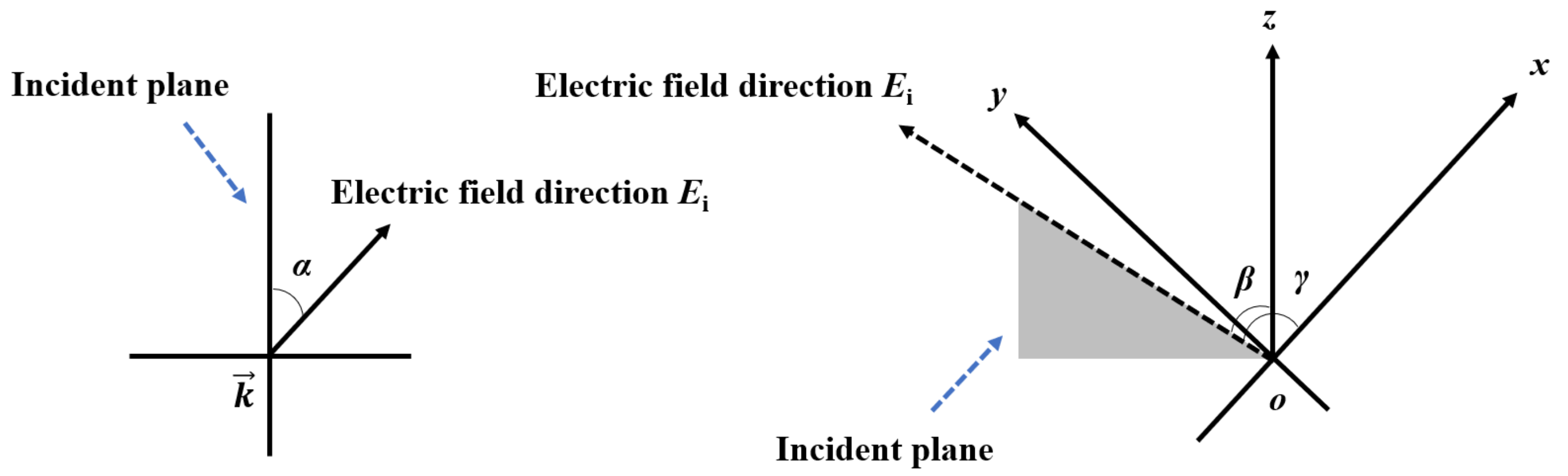
In addition to the characteristics of the radiation field, factors that affect the coupling effect are also related to the incident angle and polarization direction. As shown in
Figure 1, the radiation field in relation to the object (cabin hole, cable, antenna, etc.) defines the incident angle, polarization direction and other parameters. In
Figure 1,
is the wave vector which represents the direction of the incoming wave;
α is the polarization angle which defines the angel between the electric field direction and the incident plane;
β and
γ represent the incident angles in the spatial coordinate system.
2.2. Frequency Sweep Method Based on FEM Model
Currently, there are some numerical models that can be adopted to solve EMP issues, such as the finite difference time domain method (FDTD) [
6], the finite element method (FEM) [
7], the method of moments (MOM) [
8], the partial element equivalent circuit (PEEC) [
9], etc. However, no such numerical model can solve all EMP problems. The FEM model, which is based on the Maxwell’s equation as shown in Equation (2), is particularly suitable for solving complex structures, wide frequency domains or electrically large objects [
10]. Hence, the FEM model is adopted in this paper.
where
is the magnetic field strength of the medium, A/m;
is the angular frequency, Hz;
is the dielectric constant of the medium;
is the electric field strength, V/m.
Furthermore, the frequency sweep method based on the FEM model is carried out for the HEMP of the typical transport aircraft. For the frequency sweep method, the frequency ranges are determined according to the main characteristics of the field strength. Meanwhile, various parameters including the electric field strength distribution are calculated with Altair FEKO software. Altair FEKO is a comprehensive computational electromagnetic software that is widely used and validated in various sectors including in telecom, aerospace and defense industries. The time-domain EM solver is used to compute the voltages across, and currents through, the terminated cable ports [
11].
2.3. Geometry Model
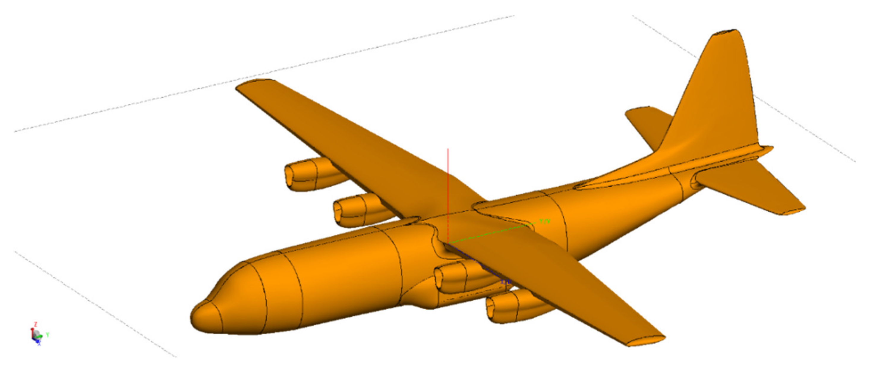
In this section, a Cartesian 3D geometry model for the transport aircraft is presented as shown in
Figure 2. In
Figure 2, the geometric aircraft model has been constructed based on the typical transport aircraft, Lockheed Martin’s LM-100J [
3]. In the case of events such as the Chernobyl nuclear power plant accident, it can act as a civil multi-purpose air freighter capable of a rapid and efficient transportation of cargo. The detail parameters of the LM-100J aircraft plane can be accessed easily. This section mainly focuses on the main structure parameters as shown below.
In order to maintain the basic structure of the aircraft, the study ignores unnecessary details such as windows. Additionally, the model is composed of all-metal materials and is therefore defined as an ideal conductor. Hence, the field strength is mainly focused and simulated around and inside the aircraft. For the dimension sizes of the geometry model of the transport aircraft, the fuselage length (x), wingspan width (y) and height (z) are x × y × z = 35.07 m × 39.48 m × 10.89 m respectively.
2.4. Numerical Setup
In this section, the cruise altitude of the transport aircraft is around 10 km and the HEMP generates at a height of about 30 km [
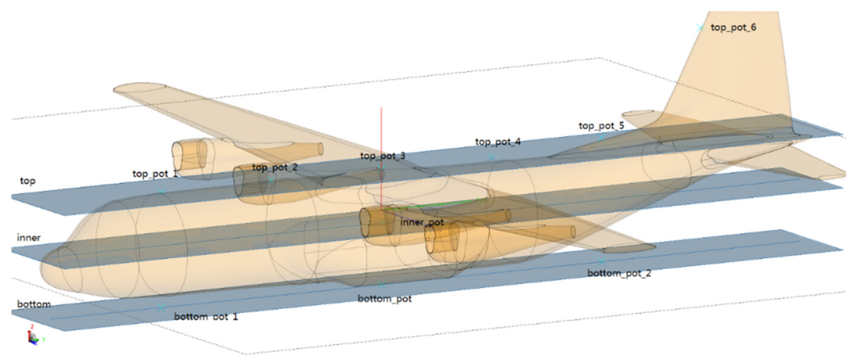
1]. In the scope of the horizon, the transport aircraft suffers from the HEMP field with a direction of oblique incidence. At the same time, the field strength solution point is set as shown in
Figure 3. In
Figure 3, the gray surface represents the layers for solving the electric field strength distribution. The three layers include: the top layer, inner layer and bottom layer.
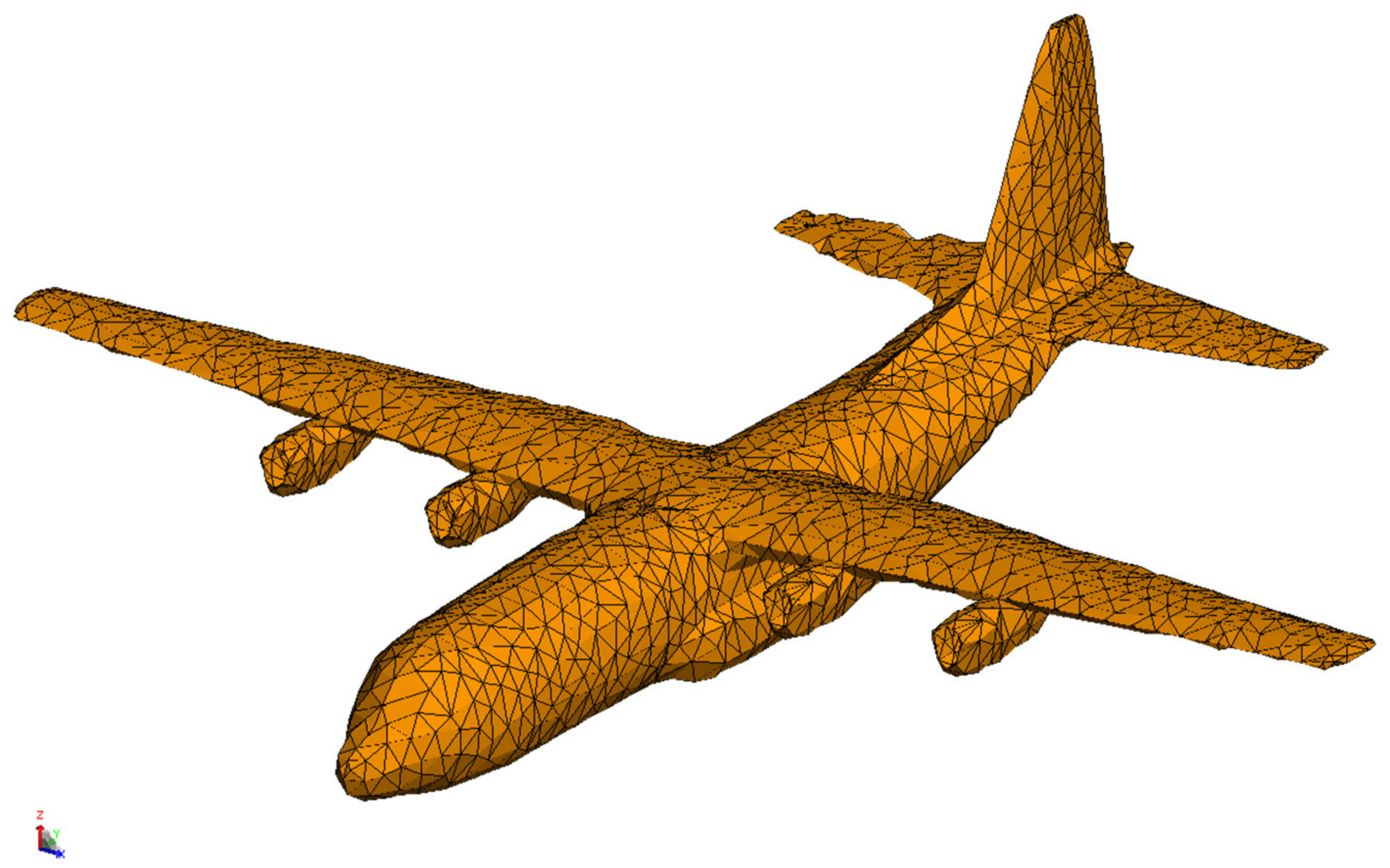
For the frequency sweep method with full-size dimensions, the main structures of the aircraft within the HEMP field are considered. Additionally, the main structures are composed of relatively complete large-size structures (such as the fuselage, the wing, and the tail). These structures are relatively simple without obvious sudden changes and electrical discontinuity. Meanwhile, the smaller and finer structures are mainly located in the engines, wing edges, and junctions of different structures. As these positions occupy a minor proportion of the aircraft geometry model, they are of less concern. Before the calculation, three mesh sizes (2941, 5882 and 11,764) are used to obtain the optimal size. For the electric field intensity
E(
t), the relative errors of
E(
t) at
t = 5 ns at a certain point are 3.9% and 0.2% respectively. To ensure accuracy and time efficiency, an appropriate mesh size of 5882 has been selected as shown in
Figure 4.
3. Results
In this section, the characteristics of the HEMP are analyzed. Then, various parameters, including the electric field strength distribution, are calculated using FEKO software. Afterwards, the electric field strength distributions of three layers (top layer, inner layer and bottom layer) are calculated and analyzed. It should be noted that this method is based on the FEM model.
3.1. HEMP Characteristics
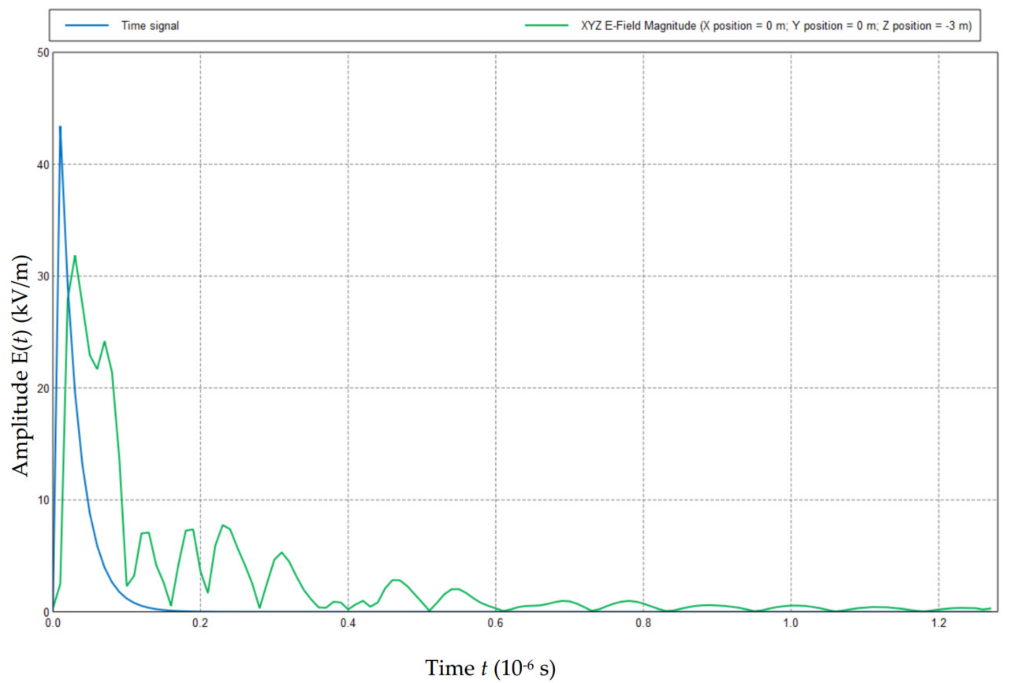
Firstly, the HEMP characteristics in the free space and at ground level are analyzed to obtain the frequency range and electric field strength distribution tendency. To save on effort and time, the amplitude of the electric field strength is set as 1 V/m in this section.
3.1.1. HEMP Characteristics with Free Space
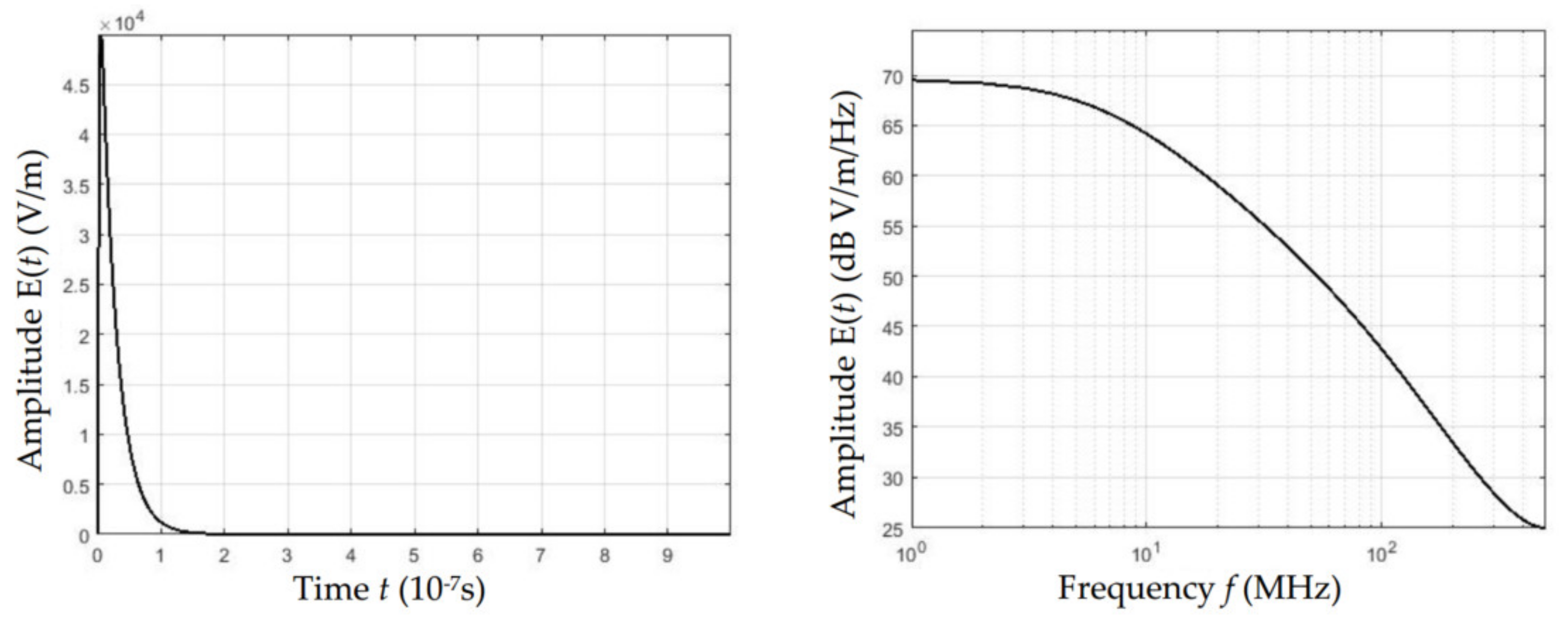
According to Equation (1), there is a double exponential pulse waveform, which has the characteristics of a short rise time, long fall time, long tailing, and a strong peak field.
Figure 5 shows the time-domain and frequency-domain waveforms of the HEMP radiation field respectively.
In
Figure 5, the EMP radiation field energy is mainly concentrated in the low frequency band (within 100 MHz), and the field strength value at each frequency point in the low frequency band is relatively uniform. These constitute the main frequency components that cause a coupling effect in the electronic equipment of the aircraft platform. If the frequency
f is greater than 100 MHz, the amplitude of the frequency components decreases at a rate of about 20 dB per decade as the frequency increases. Hence, the frequency sweep method can be considered useful for necessary calculations, and the calculation frequency range is defined as 1 kHz~50 MHz.
3.1.2. HEMP Characteristics with Ground Level
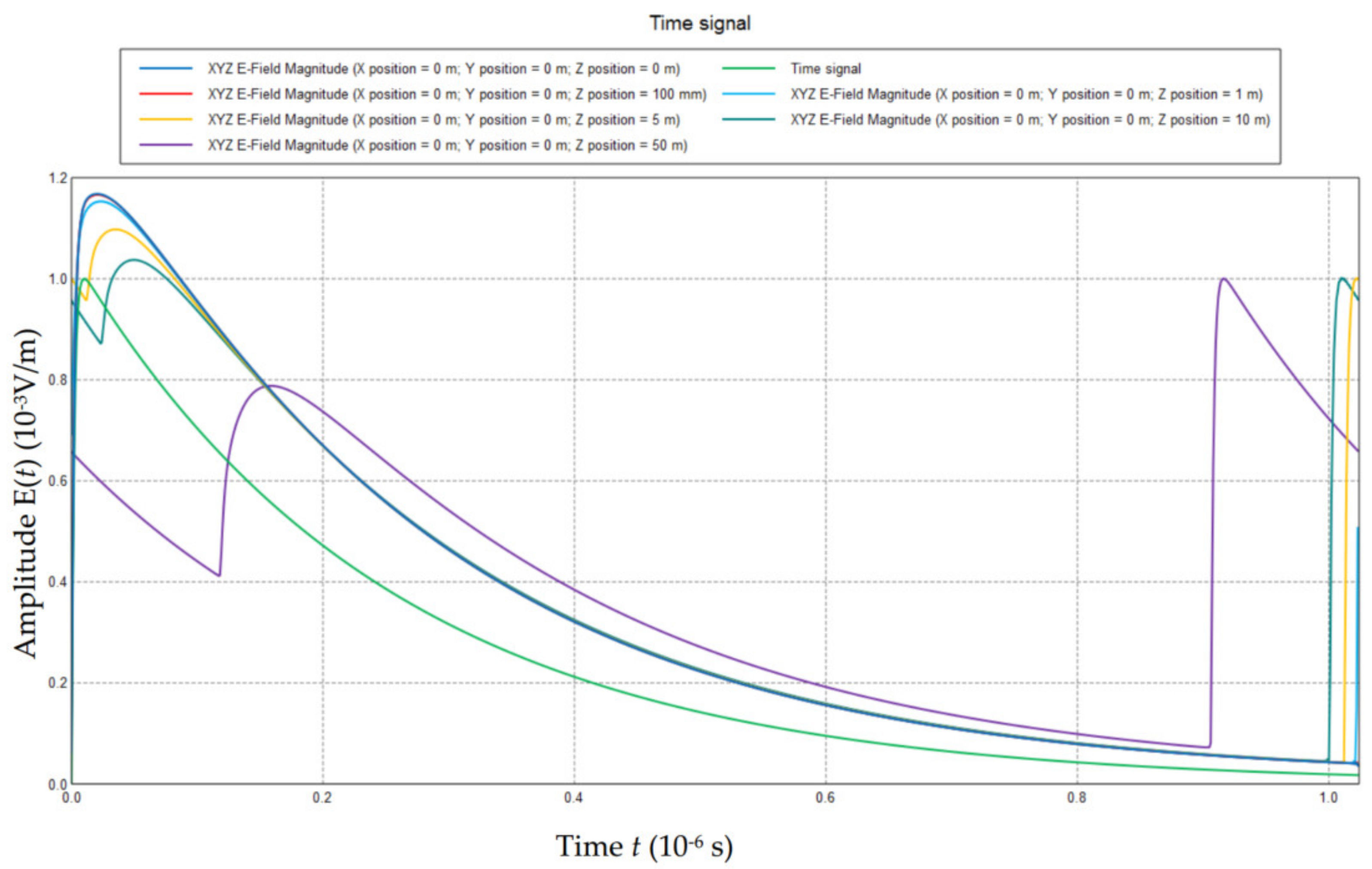
Transport aircraft commonly suffer from a HEMP with a direction of oblique incidence. In order to analyze the field intensity distribution on the ground level and in its vicinity, the polarization angle
α, the incident angles
β and
γ are set as
α = 0°,
β = 45°,
γ = 0°. Above the ground level, several positions are focused on, including
z = 0 m, 0.1 m, 1 m, 5 m, 10 m and 50 m. As shown in
Figure 6, numerical results of the electric field strength distribution
E(
t) at various values of
z outside the aircraft have been obtained.
As can be seen in
Figure 6, the electric field strength distribution
E(
t) depends on the height
z when the oblique incidence occurs. Considering the height of the object (cabin hole, cable, antenna, etc.) differs, the electric field strength distribution of three layers (top layer, inner layer and bottom layer) should be calculated and analyzed at various positions.
3.2. Magnetic Field Strength Distribution
Then, at different times,
t, the distribution of induced magnetic field strength
H formed by the HEMP radiation field on the aircraft is analyzed. In
Figure 7 schematic illustrations of the magnetic field strength
H on the aircraft at different times
t with the frequency sweep method, are presented.
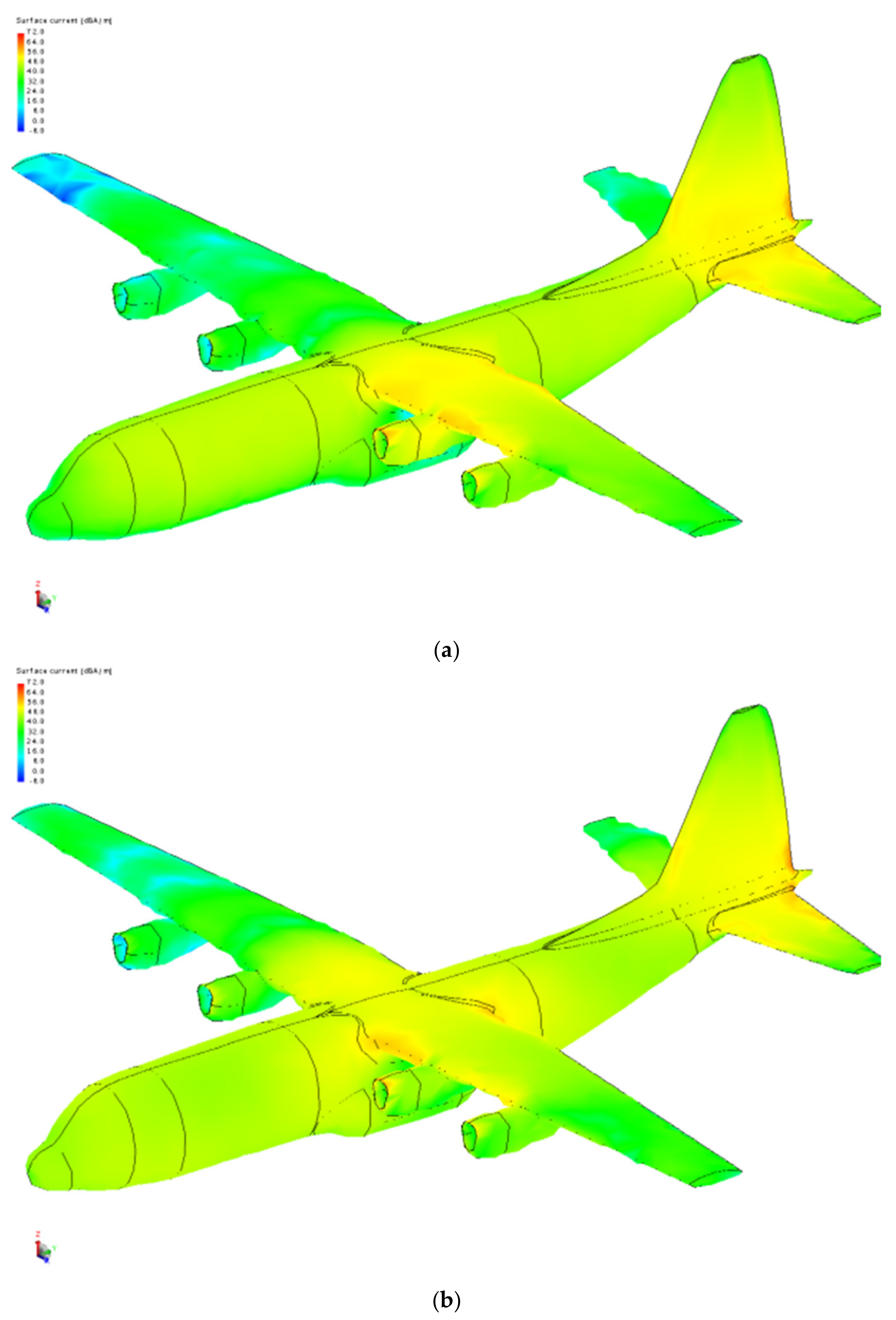
At the time
t = 0, the HEMP with the oblique incidence as the incident angle
β = 45° just reaches the aircraft. Although the electric field strength distribution
E(
t) is zero, the change rate of
E(
t), and hence the magnetic field strength
H, are quite large. Due to the oblique incidence of the HEMP field, the part of the aircraft that is far away from the incident field has not been illuminated in
Figure 7a. Therefore, the magnetic field strength distribution is formed on both sides of the wing, and is larger near the radiation field.
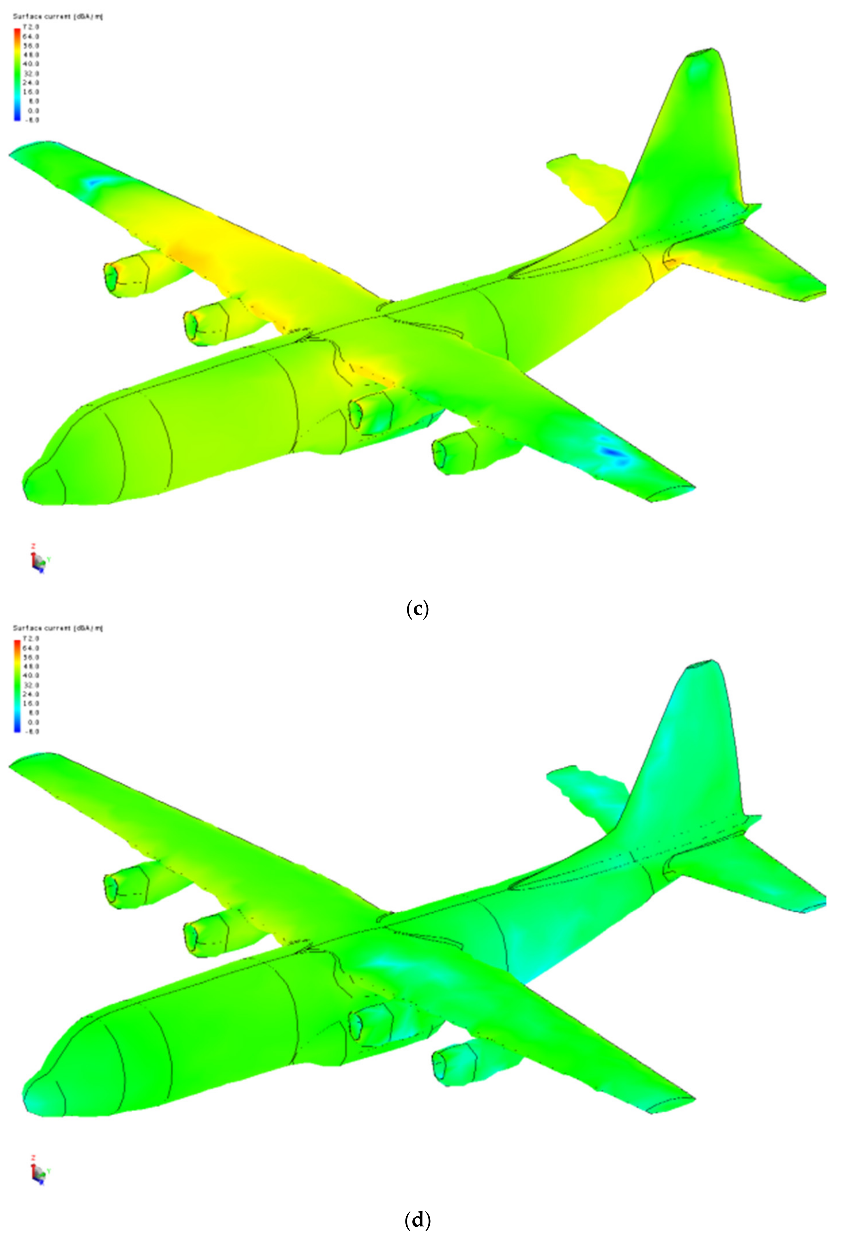
For the time
t = 10 ns, almost the entire aircraft is irradiated by the HEMP field. At this time, the field strength is the largest, and the magnetic field strength distribution is also significant. In addition, it can be seen from
Figure 7b that the magnetic field strength
H is stronger at the sharp position of the aircraft than that at other positions. In
Figure 7c,d, with the time
t increased (
t = 30 ns~400 ns), the HEMP radiation field intensity gradually decreases, and the magnetic field strength
H also gradually decreases. The order of the magnitude of the peak magnetic field strength
H is around 70 dBA/m. Therefore, the induced magnetic field strength of the aircraft is related to the HEMP radiation field strength and the change rate of the electric field strength. It is also quite large at the shape position of the aircraft which is more likely to generate the coupling effect.
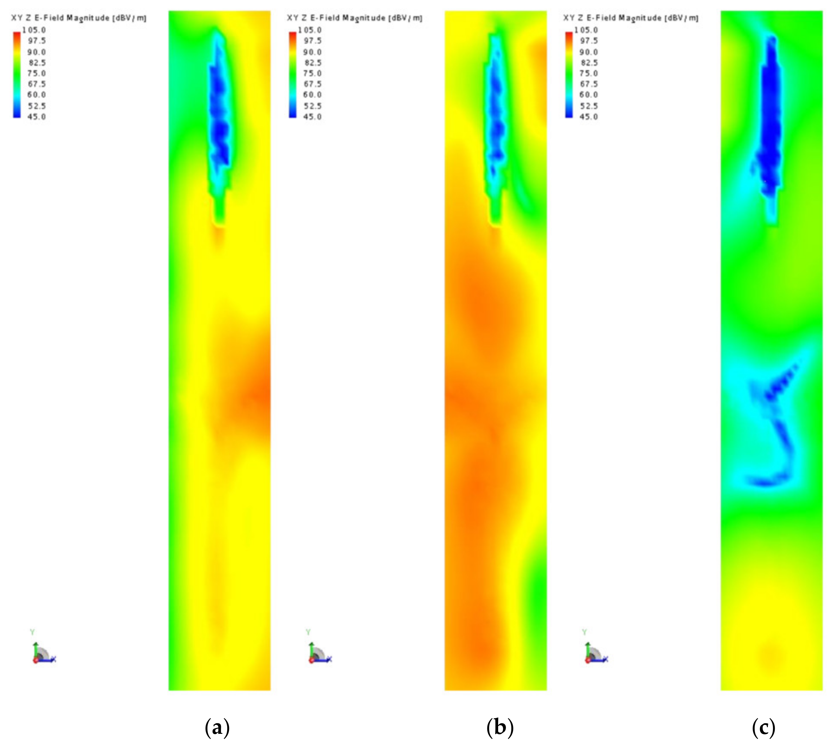
3.3. Electric Field Strength Distribution of Top Layer
Afterwards, the distribution of the electric field strength E(t) formed by the HEMP radiation field on the aircraft is analyzed. Numerical results of the top layer on or outside of the aircraft are calculated and analyzed using the frequency sweep method.
In
Figure 8a, the induced electric field strength
E(
t) of the top layer of the aircraft is found to be significant at the time
t = 0 ns.
E(
t) is uneven at the same time in
Figure 8a and
Figure 8c,. In addition, the value of
E(
t) in the internal space of the aircraft is relatively small while the peak value of
E(
t) exceeds 50 kV/m. These phenomena occur due to two reasons. On the one hand, the incidental HEMP field on the plane, at the same time measurement, is different. On the other hand, the positions of different structures of the aircraft have various reflection properties.
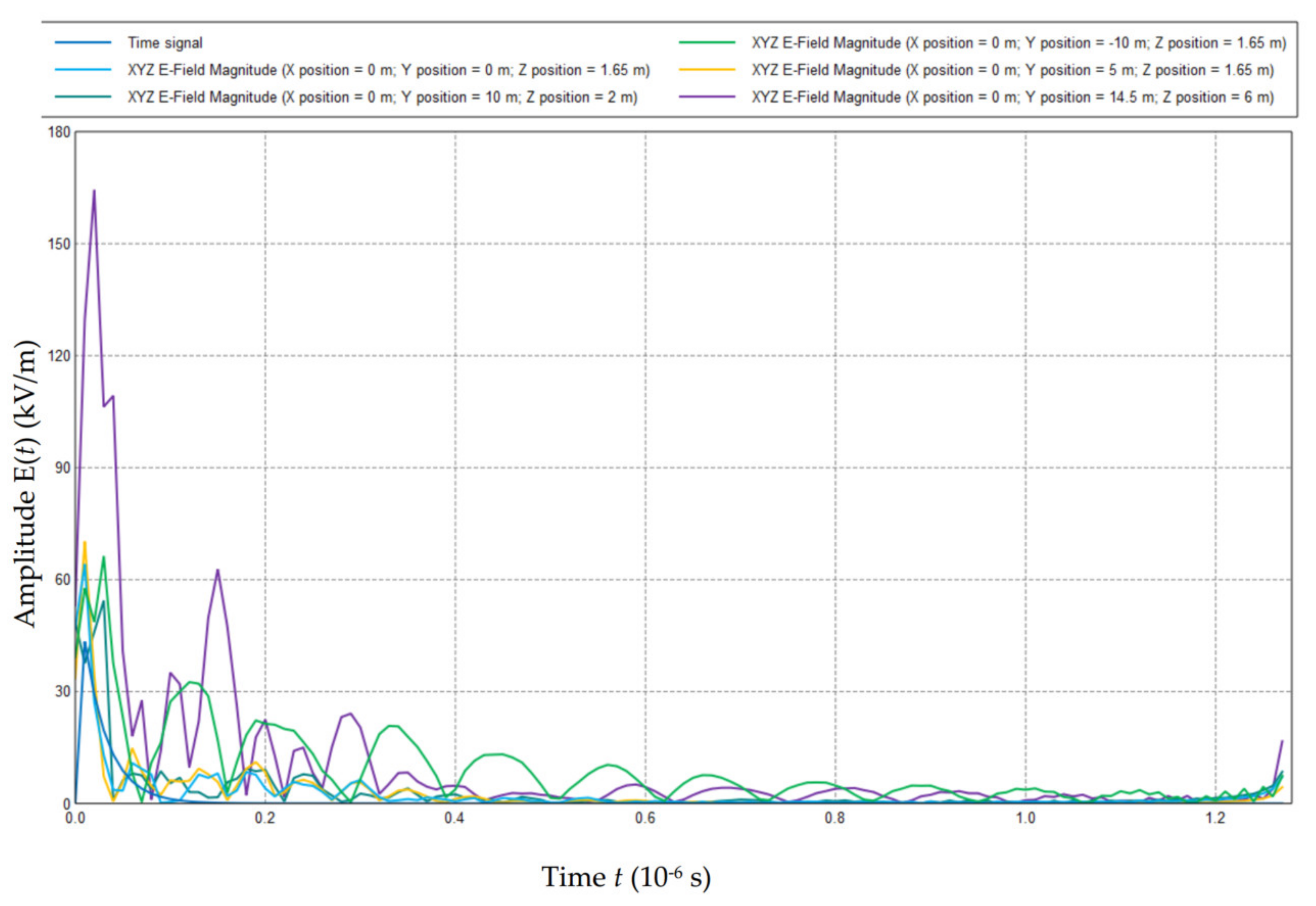
In
Figure 9, tendencies of the electric field strength
E(
t) at various positions outside of the aircraft are presented. As shown in
Figure 9, the peak value of
E(
t) which is around 155 kV/m (three times that of
E0), occurs at the position
x = 0 m,
y = 14.5 m,
z = 6 m. This position is near the back wing of the aircraft, which has a sharp structure. Due to the reflection, the electric field strength near this position
E(
t) increases significantly.
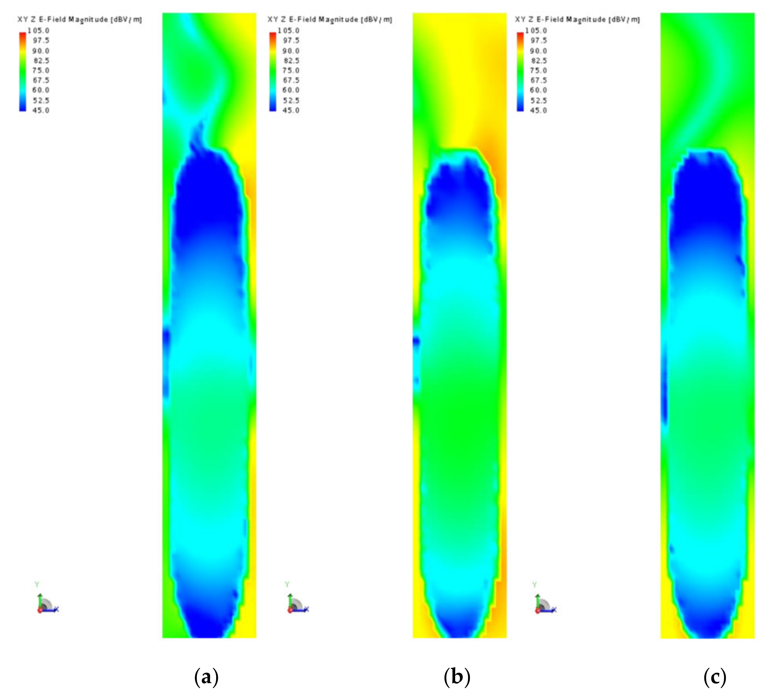
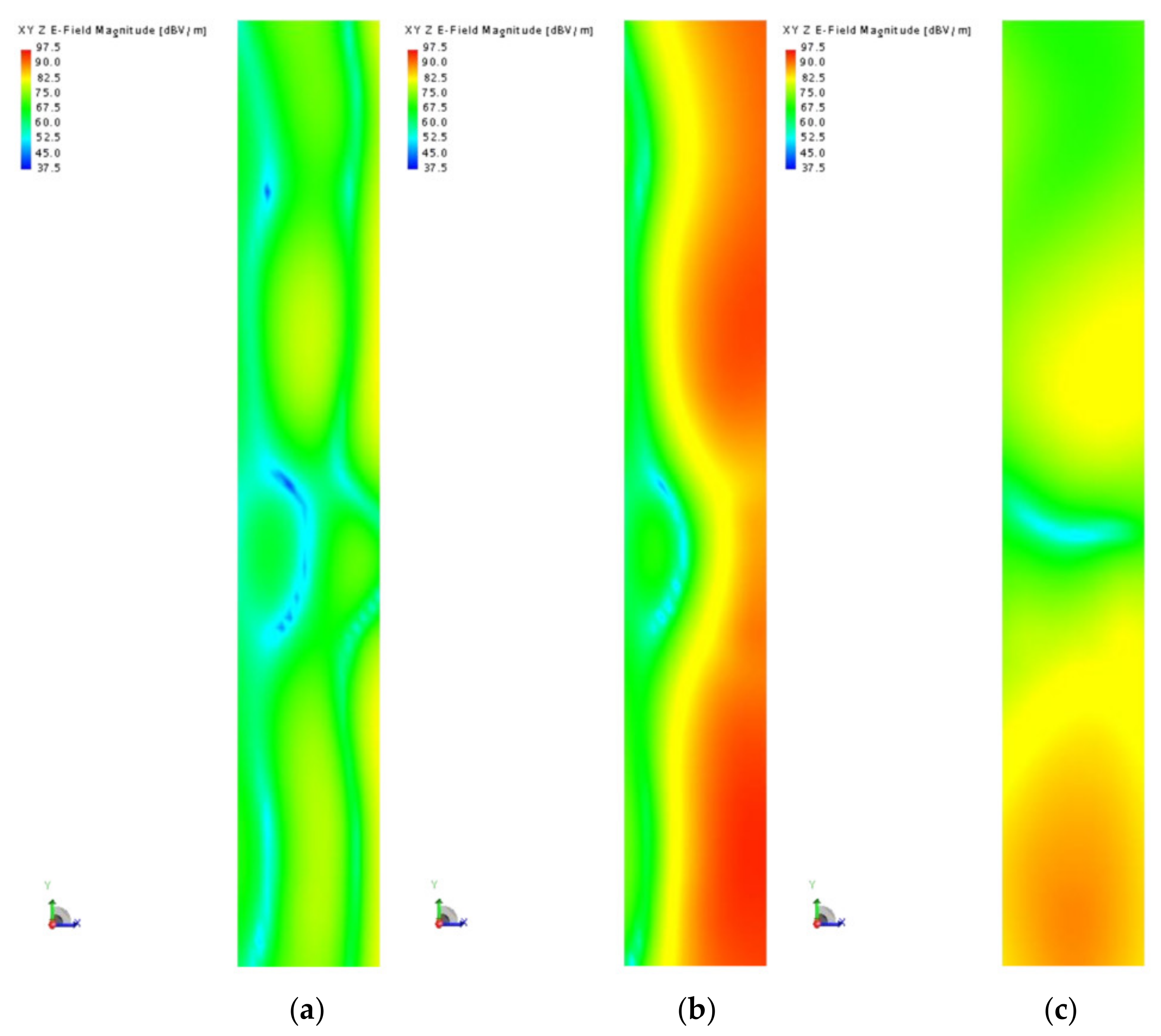
3.4. Electric Field Strength Distribution of Inner Layer
Similarly, the distribution of the electric field strength
E(
t) formed by the HEMP radiation field on the aircraft is analyzed. Numerical results of the inner layer on or inside of the aircraft are calculated and analyzed using the frequency sweep method as shown in
Figure 10 and
Figure 11. In
Figure 10, this inner layer is partly located inside the aircraft, and it can be seen that the electric field strength
E(
t) in this part is maintained at small values.
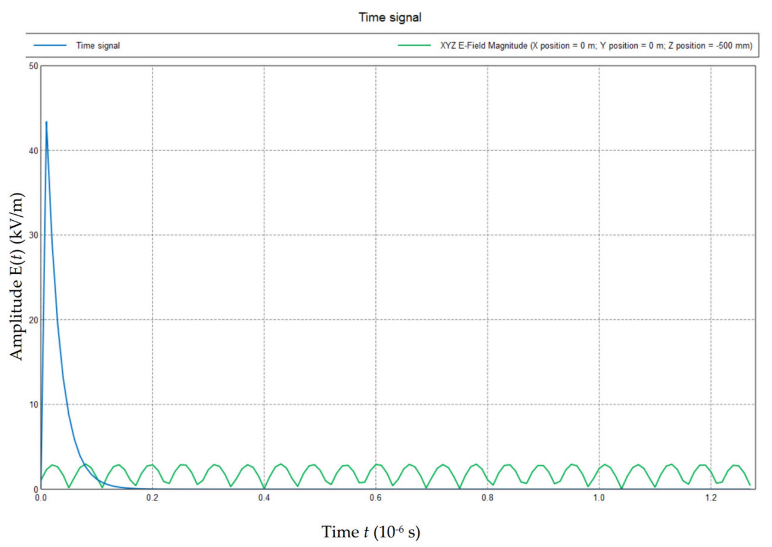
In addition, according to
Figure 11, the electric field strength
E(
t) distribution inside the aircraft oscillates with the time
t. This is due to the oscillatory effect caused by the field inside the aircraft fuselage, which forms a closed cavity. The oscillatory effect, which is reflected in this waveform, is a characteristic of the field coupling of the cavity structure.
3.5. Electric Field Strength Distribution of Bottom Layer
Lastly, the distribution of the electric field strength E(t) formed by the HEMP radiation field on the aircraft is analyzed. Numerical results of the bottom layer on or outside of the aircraft are calculated and analyzed using the frequency sweep method.
In
Figure 12, the bottom layer is below the aircraft fuselage and wings. Due to the obstruction of the fuselage and wings, the induced electric field strength
E(
t) at the bottom layer is smaller than that at the top and inner layers. However, values of
E(
t) at most locations on the aircraft are still higher than the initial value
E0 (50 kV/m).
Figure 13 displays the tendencies of the electric field strength
E(
t) at various positions of the bottom layer, outside the aircraft.
4. Conclusions
In this work, firstly, the characteristics of the HEMP radiation field are analyzed. Then, various parameters including the electric field strength distributions are calculated with FEKO software. Afterwards, the electric field strength distributions of three layers (top layer, inner layer and bottom layer) are calculated and analyzed. The main conclusions that have been reached are as follows:
Most importantly, the HEMP induced field is affected by the aircraft body. The induced electric field strength E(t) at different positions varies largely. Nevertheless, the peak value of E(t) is usually greater than the initial peak value of the electric field strength E0.
Further, the induced magnetic field strength of the aircraft is related to the HEMP radiation field strength and the change rate of the electric field strength. It is also quite large at the shape position of the aircraft, which is more likely to generate the coupling effect. The order of the magnitude of the peak magnetic field strength H is around 70 dBA/m.
In addition, the peak value of E(t) which is around 155 kV/m (three times of E0) occurs at the position of x = 0 m, y = 14.5 m, z = 6 m. This position is near the back wing of the aircraft, which has a sharp structure. Due to the reflection, electric field strength near this position E(t) increases significantly.
Furthermore, the electric field strength E(t) distribution inside the aircraft oscillates with the time t. This is due to the oscillatory effect caused by the field inside the aircraft fuselage, which forms a closed cavity.
Lastly, due to the obstruction of the fuselage and wings, the induced electric field strength E(t) at the bottom layer is smaller than that at the top and inner layers.
The results indicate that numerical calculations with the sweep frequency method based on the FEM model can reveal the characteristics of the magnetic field strength distribution and the electric field strength distribution on/inside/outside of the aircraft. T can provide guidance and insight into the necessary protection design for the HEMP of the aircraft.
Author Contributions
Conceptualization, Q.L.; formal analysis, G.H.; methodology, G.H.; investigation, G.H. and Q.L.; resources, Q.L.; writing-original draft preparation, G.H.; writing–review and editing, Q.L.; visualization, G.H.; supervision. Q.L. All authors have read and agreed to the published version of the manuscript.
Funding
This research received no external funding.
Institutional Review Board Statement
Not applicable.
Informed Consent Statement
Not applicable.
Conflicts of Interest
The authors declare no conflict of interest.
Abbreviations
| EMP | The electromagnetic pulse |
| FDTD | The finite difference time domain method |
| FEM | The finite element method |
| HEMP | The high-altitude electromagnetic pulse |
| MOM | The method of moments |
| PEEC | The partial element equivalent circuit |
| E0 | The initial peak electric field intensity, E0 = 50,000 V/m |
| E, E(t), E1 | The electric field intensity, V/m |
| f | The frequency, Hz |
| H, H1 | The magnetic field strength, A/m |
| H | The magnetic field strength, A/m |
| The wave vector |
| t | The time, s |
| x, y, z | The spatial coordinates, m |
| α | The polarization angle, rad |
| β, γ | The incident angles, rad |
| σ | The conductivity, 1/(Ω·m) |
| μ | The magnetic permeability, J/(A2·m) |
| The angular frequency, Hz |
References
- Hoad, R.; Radasky, W.A. Progress in high-altitude electromagnetic pulse (HEMP) standardization. IEEE Trans. Electromagn. Compat. 2013, 55, 532–538. [Google Scholar] [CrossRef]
- Radasky, W.A. Generation of high-altitude electromagnetic pulse (HEMP). In Proceedings of the 2008 IEEE International Symposium on Electromagnetic Compatibility, Detroit, MI, USA, 18–22 August 2008; pp. 1–5. [Google Scholar]
- Gardner, R.L.; Baker, L.; Gilbert, J.L.; Baum, C.E.; Andersh, D.J. Comparison of published HEMP and natural lightning on the surface of an aircraft. In Lightning Electromagnetics; Routledge: London, UK, 2017; pp. 491–533. [Google Scholar]
- Nanevicz, J.E.; Vance, E.F.; Radasky, W.; Uman, M.A.; Soper, G.K.; Pierre, J.M. EMP susceptibility insights from aircraft exposure to lightning. IEEE Trans. Electromagn. Compat. 1988, 30, 463–472. [Google Scholar] [CrossRef]
- Chen, C.; Wei, Y.; Yang, Z.; Enrong, W.; Chunxiao, F.; Runqing, M.; Jiaming, Z. Simulation and analysis of EMP transient electromagnetic effect of aircraft. J. Eng. 2019, 16, 2464–2467. [Google Scholar] [CrossRef]
- Gong, Y.; Hao, J.; Jiang, L.; Liu, Q.; Zhou, H. Research and application of the FETD method for the EM transient response of MTLs excited by HEMP. IET Sci. Meas. Technol. 2019, 13, 803–811. [Google Scholar] [CrossRef]
- Napolitano, F.; Borghetti, A.; Nucci, C.A.; Rachidi, F.; Paolone, M. Use of the full-wave finite element method for the numerical electromagnetic analysis of LEMP and its coupling to overhead lines. Electr. Power Syst. Res. 2013, 94, 24–29. [Google Scholar] [CrossRef]
- Kichouliya, R.; Thomas, M.J. Radiation pattern of a hybrid type high altitude electromagnetic pulse (HEMP) simulator. In Proceedings of the 2016 IEEE International Symposium on Electromagnetic Compatibility (EMC), Ottawa, ON, Canada, 25–29 July 2016; pp. 530–535. [Google Scholar]
- Weiland, T.; Zhang, M. EMC modeling for large electronic systems. In Proceedings of the 2010 Asia-Pacific International Symposium on Electromagnetic Compatibility, Beijing, China, 12–16 April 2010; pp. 520–523. [Google Scholar]
- Hyun, S.Y.; Du, J.K.; Lee, H.J.; Lee, K.W.; Lee, J.H.; Jung, C.; Kim, E.; Kim, W.; Yook, J.G. Analysis of shielding effectiveness of reinforced concrete against high-altitude electromagnetic pulse. IEEE Trans. Electromagn. Compat. 2014, 56, 1488–1496. [Google Scholar] [CrossRef]
- Pukkalla, S.K.; Subbarao, B. Study on Modeling & Simulation Analysis of Electromagnetic Pulse (EMP) Coupling to Cables. In Proceedings of the 2018 15th International Conference on ElectroMagnetic Interference & Compatibility (INCEMIC), Bangalore, India, 13–16 November 2018; pp. 1–4. [Google Scholar]
| Publisher’s Note: MDPI stays neutral with regard to jurisdictional claims in published maps and institutional affiliations. |
© 2021 by the authors. Licensee MDPI, Basel, Switzerland. This article is an open access article distributed under the terms and conditions of the Creative Commons Attribution (CC BY) license (https://creativecommons.org/licenses/by/4.0/).


