Multi-Objective Optimization for High-Dimensional Maximal Frequent Itemset Mining

Abstract

The solution space of a frequent itemset generally presents exponential explosive growth because of the high-dimensional attributes of big data. However, the premise of the big data association rule analysis is to mine the frequent itemset in high-dimensional transaction sets. Traditional and classical algorithms such as the Apriori and FP-Growth algorithms, as well as their derivative algorithms, are unacceptable in practical big data analysis in an explosive solution space because of their huge consumption of storage space and running time. A multi-objective optimization algorithm was proposed to mine the frequent itemset of high-dimensional data. First, all frequent 2-itemsets were generated by scanning transaction sets based on which new items were added in as the objects of population evolution. Algorithms aim to search for the maximal frequent itemset to gather more non-void subsets because non-void subsets of frequent itemsets are all properties of frequent itemsets. During the operation of algorithms, lethal gene fragments in individuals were recorded and eliminated so that individuals may resurge. Finally, the set of the Pareto optimal solution of the frequent itemset was gained. All non-void subsets of these solutions were frequent itemsets, and all supersets are non-frequent itemsets. Finally, the practicability and validity of the proposed algorithm in big data were proven by experiments.

1. Introduction

The big data association rule analysis was mainly finished in two steps. First, all frequent itemsets whose frequency of occurrence exceeded the threshold were recognized from the database. Second, all association rules that meet the minimum confidence threshold are produced by frequent itemsets. The mining of frequent itemsets is the key difficulty in association rules analysis because the overall performance in the mining of association rules is mainly determined by the performance in the first step.

The mining of frequent itemsets aims to find itemsets whose frequency of occurrence exceeds the preset frequency threshold of the given mass transaction sets. The given transaction sets correspond to the object of big data. The occurrence frequency of an itemset is called the support degree, and the given frequency threshold is called the minimum support threshold. The mining of the frequent itemset can present variables that often occur together in transaction sets, which provide support for possible decisions. The mining of frequent itemsets is also the basis of various important data mining tasks, such as correlation analysis, causal relationship, sequence itemset, local periodicity, and plot fragments. For example, in their story of beer and diapers, Walmart found that beer and diapers were often bought together through big data analysis, which indicates that beer buyers often need to buy diapers, or diaper buyers often also buy beer. Thus, frequent itemsets, such as shopping basket data analysis [1], webpage prefetching [2], cross-shopping [3], personalized websites [4], and network intrusion detection [5], have been extensively applied.

The mining algorithms of frequent itemset can generally be divided into two types, namely accurate and heuristic algorithms. The most classical accurate algorithms include Apriori [6], FP-Growth [7], and many derived algorithms [8,9,10,11,12,13,14,15,16,17,18,19,20]. The theory of accurate algorithms seems to be perfect. However, they are inapplicable to big data and high-dimensional transaction sets. The fundamental causes include the serious consumption of time and storage capacity due to the exponential explosive growth of solution space and the consequent abundant candidate itemsets and complicated data structure. Therefore, many researchers began to consider applicable heuristic algorithms. For example, the evolutionary computation and swarm intelligence algorithm were applied to solve problems [21,22,23,24,25,26].

If frequent itemsets are explored by the evolutionary algorithm, then an itemset can be used as an individual of the solution space. Many individuals form a population that is optimized in the iteration. Compared with accurate algorithms, the evolutionary algorithm might not be the best, but it can avoid the explosive solution space, thereby making the time and storage space acceptable in the face of big data and high-dimensional data.

Many studies have applied many particle swarm optimization (PSO) and genetic algorithms in heuristic algorithms to solve the mining frequent itemset. Zhang et al. [21] designed a binary PSO to mine frequent itemsets. This algorithm could cut the relieved pressure over storage and CPU time dynamically in the process of population initialization and evolution. It has also been applied to four different transaction sets. Among these four transaction sets, the number of transactions in one set was 500, and the number of transactions in the three other sets were 1000. Bagui et al. [22] applied the genetic algorithm to explore the frequent itemset in the data stream; it is novel that the conceptual drift was determined by frequent itemsets. The number of dimensions and transactions was not very high because the objects use some data within a slipping window frame of data flow. Paladhi et al. [23] designed an artificial cell division algorithm, which was very successful in solving multi-channel spatial searching tasks and was superior to the Apriori algorithm with respect to small-scaled transaction sets. Chiu et al. [24] applied the PSO algorithm to explore a frequent itemset from a transaction set named FoodMart2000. This FoodMart2000 transaction set contained 12,100 transactions and had 34 dimensions (number of items). Ykhlef et al. [25] explored frequent itemset in nursery transaction sets by using the quantum group evolutionary algorithm. The number of nursery transactions and dimensions were 12,960 and 32, respectively. Kabir et al. [26] strengthened the random searching performance of the PSO algorithm and explored the frequent itemset in a transaction set, which has 1000 transactions and 5 dimensions.

None of the aforementioned algorithms have been applied to high-dimensional and mass transaction sets. To test the feasibility of the algorithms, accident and marketing transaction sets of real business supermarkets were selected as the testing objects of the high-dimensional mining of frequent itemsets in this paper. The number of transactions and dimensions in accident transaction sets were 340,183, and 468. The transaction length of the accident transaction set had uniform distributions accompanied by a high quantity of transactions and dimensions. This accident transaction set was as representative and could be used as the test object. The transaction set of the business supermarket contained 65,435 marketing records, which were equal to 18,548 transaction sets. The dimension of commodities was even as high as 5547.

Although Weka [27] was the most famous software tool of ML and DM tasks, its algorithm can either be directly applied to a dataset through its interface or used in ones’ own Java codes. However, it is inapplicable to big and high-dimensional data, and the operation time cannot wait. KEEL [28] also provided many existing algorithms and testing data that are only applicable to data-type transaction sets and are thus inapplicable to the frequent item mining of Boolean-type transaction sets.

In order to mine all frequent itemsets, maximal frequent itemsets are important. If the maximum frequent itemsets are used as the search targets of the algorithm, the algorithm can find as many frequent itemsets as possible with fewer targets. This is because maximal frequent itemsets contain frequent itemsets at their maximum capacity, and all subsets of maximal frequent itemsets are still frequent itemsets. The definition of maximal frequent itemsets is given in Section 2.

In addition, relaxed functional dependencies (RFDs) are properties expressing important relationships among data [29]. Thanks to the introduction of approximations in data comparison and/or validity, they can capture constraints useful for several purposes, such as the identification of data inconsistencies or patterns of semantically related data. Nevertheless, RFDs can only provide benefits if they can be automatically discovered from data. Loredana Caruccio [30] presented an RFD discovery algorithm relying on a lattice structured search space, previously used for FD discovery, new pruning strategies, and a new candidate RFD validation method. An experimental evaluation demonstrates the discovery performances of the proposed algorithm on real datasets, also providing a comparison with other algorithms.

The remainder of this paper is as follows. Section 2 introduces the related concepts, including association rules, frequent itemsets and maximal frequent itemsets, the mathematical description of the problem and so on. Section 3 states the operating framework of the proposed algorithm and the details of each part. In Section 4, two experiments are used to illustrate the effectiveness of the algorithm. Section 5 discusses the advantages and disadvantages of the algorithm and gives the conclusion.

2. Related Concepts

2.1. Association Rules

Association rule mining is an important branch in big data and data mining technology. The concept of association rules is proposed to search the relations of data in the transaction database. Such relations are defined as association rules, such as A ⇒ B, where A and B both are sets of items (itemsets). A is called the former item of association rules, and B is the rear item of association rules. If D = {T₁, T₂, T₃, …, T_k} is the big data transaction set that is used to extract the association rule, then T_i = {I_i1, I_i2, I_i3, …, I_ik} is a transaction in the transaction sets. If I = {I₁, I₂, … I_m} is the set of all items, then T_i is the non-void subset T_i ⊆ I of I. If A ⇒ B is a rule, then A ⊂ I, B ⊂ I, and A ∩ B = Ø. In association rule mining, the support degree (support) and confidence (Confidence) are used to measure the quality of one association. These two parameters are defined as

$$support\left(A\Rightarrow B\right)=P\left(A\bigcup B\right)$$

(1)

$$confidence\left(A\Rightarrow B\right)=\frac{P\left(A\bigcup B\right)}{P\left(A\right)}$$

(2)

where P(X) is the probability of occurrence (support) of the itemset X in the objects D of transaction sets. Thus, the support and Confidence of the corresponding association rule A ⇒ B could be derived if P(A ⋃ B) and P(A) are known, and whether association rules are strongly correlated can be determined. Hence, the problem of exploring the association rules can be summarized as the exploration of a frequent itemset.

2.2. Frequent Itemset

The mathematical description of frequent itemset mining is detailed as follows: based on the above text, D = {T₁, T₂, T₃, …, T_n} was set as the big data transaction set for mining, and I = {I₁, I₂, …, I_m} was the set of all items. If a set X ⊂ I is composed of several items and the probability of occurrence (P(X)) of X in the transaction set T_i of D is higher than the preset threshold, then X is called the frequent itemset. |X| expresses the number of items in the itemset. If |X| = k, then it is called the k-itemset. Given a minimum support threshold (min_supprot), the frequent itemset mining aims to find all the frequent itemsets whose support is higher than the threshold. Based on this definition, the following properties can be determined:

Property 1.

Given any non-void itemset X, Y ⊆ I, support (X) ≥ support (Y) if X ⊆ Y. Therefore, X is the frequent itemset if Y is a frequent itemset, and Y is not a frequent itemset if X is not a frequent itemset.

Definition 1.

Closed frequent itemset. When the itemset X is a frequent itemset and no superset Y of X is found in the transaction sets D to make support (X) = support (Y), then X is a closed frequent itemset. The closed frequent itemset expresses lossless compression and has no loss of information about support. All frequent itemsets and corresponding supports can be obtained from the closed frequent itemset through the inversion mode.

Definition 2.

Maximal frequent itemset. If the itemset X is a frequent itemset and any superset of X is not a frequent itemset, then X is a maximal frequent itemset. The expression of the maximal frequent itemset is a lossy compression, and it loses information about the support of the frequent itemset. Whether an itemset is frequent can be judged according to the maximal frequent itemset. However, the corresponding supports cannot be obtained.

2.3. Mathematical Description of Multi-Objective Optimization of Maximal Frequent Itemset Mining

The maximal frequent items were used as the optimization objective. Then, two optimization objects, namely support and the number of items in an itemset, were noted. According to Property 1, support and the number of items in an itemset are two contradictory optimization objectives. The constraint was that the support was higher than the given threshold. Given the gene codes of solution individual X = (x₁, x₂, …, x_m) and big data transaction set D, the mathematical descriptions of the multi-objective optimization problem are:

$$Maximize P\left(X\right)$$

(3)

$$Maximize {{\displaystyle \sum }}_{i=1}^m{x}_i$$

(4)

$$\begin{array}{cc}s.t.& \begin{array}{c}P\left(X\right)\ge min\_support\\ x_i\in \left\{0,1\right\}\left(i=1~m\right)\end{array}\end{array}$$

(5)

where P(X) is the probability of occurrence of an itemset, which is determined by the individual gene encoded in D, which is known as support. m is the quantity of the frequent 1-itemset with support higher than the threshold. X_i ∈ {0, 1} (i = 1, 2, …, m) is a decision variable that is used to determine whether the item i belongs to the itemset X, where 0 indicates no and 1 indicates yes. Min_support is the support threshold that is used to determine whether it belongs to the frequent itemset. If P(X) is not lower than the threshold, then it is a frequent itemset; otherwise, it is not a frequent itemset.

3. Multi-Objective Optimization of Maximal Frequent Itemset Mining

Frequent itemset mining aims to find all frequent itemsets that meet the threshold requirements. According to Property 1, if all maximal frequent itemsets can be found, then all their nonempty subsets are frequent itemsets, and all frequent itemsets are found. Therefore, the designed mining algorithm proposes an evolutional computation method of multi-objective optimization (MOO) to search for a maximal frequent itemset from the high-dimensional transaction sets by using the maximal frequent itemset as the search objective and high-dimensional transaction sets as the objects.

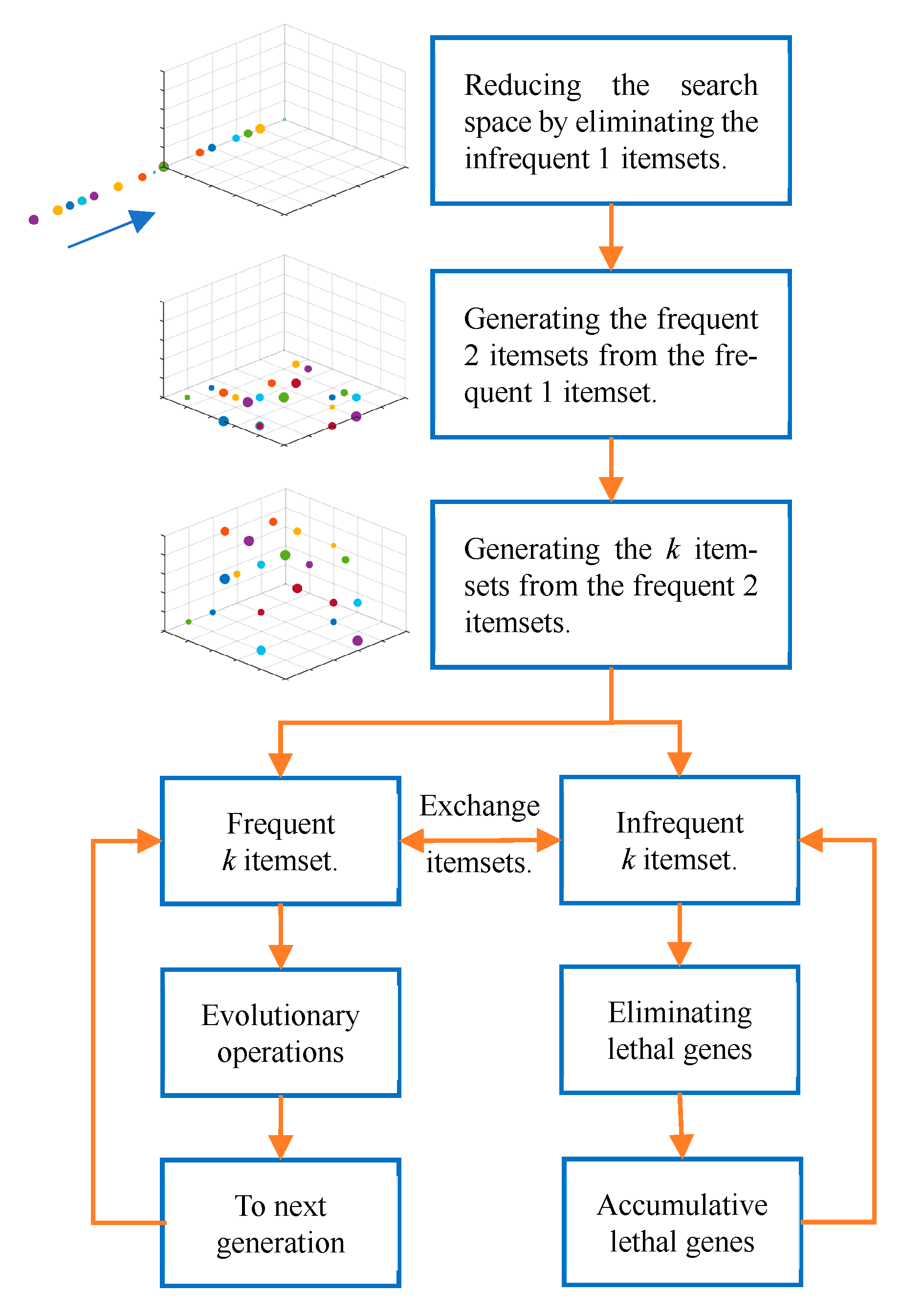
3.1. Working Diagram of MOO

The operation principle of MOO is shown in Figure 1. According to the given high-dimensional transaction sets and minimum support, ① the transaction sets were scanned first to eliminate all non-frequent 1-itemsets that would not participate in the follow-up calculations; ② the remaining frequent 1-itemsets were used to construct all possible 2-itemsets and the 2-itemsets with support smaller than the minimum threshold were deleted; ③ a different number of frequent 1-itemsets were randomly added into each of the remaining frequent 2-itemsets, which gained the same quantity of k-itemsets with the frequent 2-itemsets; ④ the support of each k-itemset was evaluated, and these k-itemsets were divided into two groups according to the support threshold. The group with support higher than the threshold was used as the frequent itemset, which was recorded as group 1. Another group was used as the non-frequent itemset, and it was recorded as group 2; ⑤ group 1 was used as the population of multi-objective optimization, and generations of alterative iterations of multi-objective optimization were performed; ⑥ according to the accumulated lethal gene library, gene repair was performed to each individual of group 2. Then, encoded genes were recorded, and the lethal gene library was updated; ⑦ individuals in group 1 and group 2 were exchanged, and non-frequent itemsets in group 1, which were produced from multi-objective optimization, were moved to group 2. The resurgent individuals in group 2 were moved to group 1. Then, they were returned to step ⑤ and successively circulated until the end of the iteration.

The operation of an algorithm involves some detailed problems such as individual gene encoding design, fitness function, and the use of reduced transaction sets and repair operators of individual genes of non-frequent itemsets. These problems were introduced in the following texts.

3.2. Individual Gene Encoding

Evolutionary objects, which form the population during multi-objective optimization, were called individuals. The composition form of individuals was called the gene encoding mode. One gene encode corresponds to one solution, which is called one itemset. The algorithm deletes all 1-itemsets with support smaller than the threshold, so the remaining m frequent 1-itemsets with support higher than the threshold were left. To save spaces, the remaining items with support higher than the threshold were renumbered from 1 to m. Then, the individual encode in this study was an m-dimensional binary vector:

X = (x₁, x₂, …, x_m)

(6)

One itemset is also expressed by individual gene encodes. x_i ∈ {0, 1} (i = 1, 2, …, m) expresses whether the item i is a member of the itemset after renumbering. If its value is 0, then the item i is not a member of the itemset. If its value is 1, then the item i is a member of the itemset. m is the number of the frequent 1-itemsets and the length of genes. If we let k = ∑x_i, then k items are found in one itemset. Therefore, the gene encodes corresponds to one k-itemsets.

3.3. Using Reduced Transaction Sets

To accelerate the assessment on the execution speed of the fitness function of individuals, the algorithm deletes all 1-itemsets with support smaller than the threshold in step ① of the operation framework while updating the transaction set. Each transaction in the transaction set also deletes all non-frequent items (1-itemset) and generates one new transaction set. In this way, the target transaction set was not only significantly reduced in horizontal and longitudinal directions without changing any computation results but also increases the computational speed and complexity. In the future operation of the algorithm, all operators use the new transaction set to substitute the object transaction set. The reason is that the disposal scanning of transaction set hardly increases the execution time and complexity of the algorithm but it significantly improves the evolutionary and execution speed of the fitness function.

3.4. Fitness Function

The algorithm deletes all 1-itemsets with support smaller than the threshold in step ①, which actually significantly decreases the dimensions of searching space. Based on Property 1, all follow-up searching tasks are performed in the m-dimensional space because all the multi-itemsets that contain non-frequent 1-itemsets cannot be frequent itemsets.

In the selection mechanism of the survival of the fittest in multi-objective optimization, the quality of individual encodes was assessed by the fitness function. The individual encodes correspond to one itemset, and the support of the itemset can reflect the quality of individuals. The number of items of the itemset is an objective of the algorithm because it searches the maximal frequent itemset or the itemset that contains items that meet the support threshold as much as possible. Hence, the product of support and number of items in the itemset was used as the evaluation function of individual encodes.

Given the reduced transaction set D = {T₁, T₂, T₃, …, T_n}, T_i = (t_i1, t_i2, …, t_im), t_ij ∈ {0, 1}, (i = 1, 2, …, n), (j = 1, 2, …, m). The evolutionary individual encodes X = (x₁, x₂, …, x_m), x_i ∈ {0, 1} were provided. It hypothesized that the itemset determined by the binary individual encodes X was A, and the pseudo-code Algorithm 1 of the fitness of the evolutionary algorithm of the individual X was calculated.

Algorithm 1 Giting fitness

Input: D = (T1, T2, …, Tn), X = (x1, x2, …, xm), A Output: A new X and it’s Fitness length = ${{\displaystyle \sum }}_{i=1}^m{x}_i$; fitnesss = 0; f = 0; (r1, r2, …, rm) = (0, 0, …, 0); for i = 1: n do   Continue with some probability;   If A ⊆ Ti; then     fitness = fitness + 1;     for j = 1: m do       rj = rj + tij;     end   end   f = f + 1; end for j = 1: m do   if ri/f > SupportThreshold then     rj = 1;   else     rj = 0;   end end if ${{\displaystyle \sum }}_{i=1}^m{r}_i$ > length then   select xk = 0 with rk/f > SupportThreshold;   xk = 1;   fitness = rk/f*(length + 1); else   fitness = fitness/f*length; end Retrun fitness;

where “Continue with some probability” is an operation of skipping over the “for” loop at a certain probability, which can shorten the execution time of the fitness function. In fact, this step replaces the sampled transaction sets by the real reduced transaction set D and the sampled transaction sets distribute uniformly in D. This again significantly reduces the time complexity of fitness function, and it would not influence the evolutional computation mechanism of the survival of the fittest. It was feasible in this algorithm.

The calculation of the fitness function involves two tasks. First, it adds one item into the itemset based on no changes to the frequency (whether support is still higher than the threshold), and no item is added if the itemset is a maximal frequent itemset. Second, the product between the support of the new itemset and the number of items is returned. The returned value of the fitness is composed of supports of two factors and the number of items. On the one hand, the support of the itemset was investigated. On the other hand, the number of items in the itemset was considered. This was caused by the optimization objective of the maximal frequent itemset.

3.5. Individual Gene Repair

In the middle and late stages of algorithm evolution, the support declines because of the increase in the items of evolutionary individuals, and the supports of abundant individuals are close to the threshold. Under the disturbance of evolutionary operators, many non-frequent itemsets were generated using the rigid threshold. Individuals of these frequent itemsets in the evolutionary algorithm are called lethal chromosomes, which are abandoned in traditional evolutionary algorithms. However, these lethal chromosomes contain excellent genes after several generations of evolution. Moreover, abandoning these individuals means leaving evolutionary fruits. If the genes of lethal chromosomes can be slightly repaired, then this can promote the evolutionary performance of the algorithm. In this study, a method for repairing these lethal chromosomes was proposed.

The individual encodes of the non-frequent itemset known as the lethal chromosome X = (x₁, x₂, …, x_m) were given, and the probability vector of the frequent 1-itemset was set as p = (p₁, p₂, …, p_m). One item with x_i ≠ 0 was selected according to the probability of (1 − p_i) and set as 0. The individual X might be resurged (support higher than the threshold). The pseudo-code of the repair operator was introduced in Algorithm 2.

Algorithm 2 Repairing Operation

Input: X = (x1, x2, …, xm) with P(X) < threshold Output: Repaired X with P(X) >= threshold Select an item k with probability (1 − pi); while xk = 0 do   Reselect an item as xk = 1 with probability (1 − pi); end xk = 0;

4. Case Studies

In this study, two representative high-dimensional transaction sets were used to test the feasibility of the algorithm. One was the accident transaction set, which involved 340,183 transactions downloaded from http://fimi.uantwerpen.be/data/ (accessed on 28 February 2020). The other was the real sales data of a general supermarket in southeast China during a certain period, and the dimension of the commodities was 5547. For these two transaction sets, one has a high quantity of transactions, and the other has a high dimension of items.

The experimental hardware environment was a Mi notebook Pro 16.6”, which was composed of Intel(R) Core (TM) i7-8550U CPU @ 1.80 GHz ~ 2.0 GHz (8 CPUs) and memory: 16384MBRAM. Timi Personal Computing Limited, Beijing, China.

4.1. Accident Transaction Set Test

As stated previously, the accident transaction set covered 340,183 transactions and 468 dimensions. The transaction length of the accident transaction set has uniform distributions, a high quantity of transactions and high dimensions. It is representative and can be used as the testing objects.

The proposed algorithm cannot be compared with existing traditional algorithms in optimization, which targets the maximal frequent itemset because of two reasons. First, traditional algorithms are generally unworkable with high-dimensional big data. Second, existing algorithms have hardly used a maximal frequent itemset as the searching objective. Thus, the number of frequent itemsets that were identified by the algorithm in each iteration under the constraint of appropriate support thresholds, as well as the proportion of maximal frequent itemsets, were only investigated in this study. On this basis, the feasibility of the proposed algorithm was analyzed.

The CPU time for 100 generations of algorithm operation was 23,931 s (more than 6 h). Various results of algorithm operation are shown in Figure 2. The x axis in Figure 2a shows the number list of 468 items, and the y axis is the support of the corresponding item used as the 1-itemset. Clearly, the probability distribution of the occurrence of a single item in the transaction set was relatively uniform, and the maximum support was even close to 1. This finding indicates that this item occurs in almost every transaction, and it is the major cause of accidents if used in traffic accident association analysis.

For the purpose of the experiment, approximately 5% of the items were intercepted as the frequent 1-itemset. Therefore, it was relatively appropriate to set the support threshold as 0.5, which can intercept 24 frequent 1-itemsets. All non-frequent 1-itemsets were deleted when generating the reduced transaction sets, and the average length (number of items) of all objects was decreased from the original 33.8 to 12.3. The number of transactions in the reduced transaction set was not decreased because the support of the highest single item in the target transaction set was almost close to 1. If the algorithm was applied to other transaction sets (e.g., the supermarket data in the following text), then the quantity of transactions significantly decreased, which reduced the complexity of the algorithm in the assessment of each evolutionary individual. All frequent 1-itemsets were combined in pairwise, and a total of 24 × 23/2 = 276, 2-itemsets were generated. The histogram of support is shown in Figure 2b. The number of frequent itemsets with support higher than the threshold was 168. The algorithm randomly increased items based on these 168 frequent 2-itemsets to generate the initial population for evolution. The population scale was also set as equal to the number of frequent 2-itemsets, which was 168.

The number of frequent itemsets that are searched in each generation of the evolutionary process is shown in Figure 2c. Among them, the maximal and non-maximal frequent itemsets are available. The solution space is very large (2⁴⁶⁸), and the number of all frequent itemsets cannot be verified because this dataset is high dimensional. In this experiment, the evolution was performed for 100 generations to show the feasibility. Clearly, the number of frequent itemsets searched in each generation generally decreased with the increase in evolution generations. The number of all frequent itemsets that was obtained with the increase in evolution generations is shown in Figure 2d. The curves in Figure 2d are integrals of the function of Figure 2c at zero. After 100 iterations, at least approximately 500 frequent itemsets—including 168 maximal frequent itemsets—were gained. In fact, 216 maximal frequent itemsets exist when the threshold is set to 0.5. In other words, 77% of maximal frequent itemsets were obtained through 100 generations of evolutions. A total of 216 maximal frequent itemsets were gained in one of our papers on accurate algorithms, which aims to search for the maximal frequent itemsets (right-hand side expanding algorithm for maximal frequent itemsets mining).

Two curves are seen in Figure 2e. The upper curve shows the average number of items in each frequent itemset, which is searched in each generation and fluctuates around 10. The lower curve is relatively complicated and was set to d if the average number of items in the frequent itemsets which are searched in each generation was a. For each frequent itemset, the items which are absent in many itemsets can independently be added into the itemsets and these itemsets are still frequent (b). If the mean of b in each generation was c, therefore, d = 1 + a − c. In other words, all frequent itemsets which were searched from the current generation when d = 1 can be added with one item and the number of the frequent itemset was still zero. There is no item which can be added in. All frequent itemsets are maximal frequent itemset. It can be seen from the lower curve that the d value fluctuates around 1, which is a normal phenomenon.

There are two curves in Figure 2f. The upper one is the number of non-frequent itemsets which are encountered in each generation of searching tasks. Since the population is 168, the number of the non-frequent itemset fluctuates around 150. The sum of the number of non-frequent itemsets and the number of frequent itemset in Figure 2c is basically consistent with population size. The lower curve represents the number of frequent itemsets that are searched from each generation and which are the same with previously identified frequent itemsets. The algorithm deletes these overlapping itemsets.

In the many traditional algorithms, the two most classical ones are the Apriori and FP-growth algorithms. We know that FP-growth is faster than Apriori, which is also widely recognized. In order to compare with our algorithm, we also tested the FP-growth algorithm on the Accidents transaction set. Similarly, when the support threshold was set to 0.5, there was no result for FP-growth to mine the Accidents within 24 h.

In order to estimate the running time of the FP-growth algorithm on Accidents, the number of transactions and the length of each transaction were reduced. Some transaction were taken out of the Accidents set, such as 100, 200, etc. Only 10%, 20% and 30% of the beginning of each transaction was taken, respectively. The running time of the algorithm is shown in

Table 1. FP-growth for the extracted accidents.

	100	200	300	400	500
10%	13.916395 s	26.744861 s	25.966303 s	33.145599 s	46.008133 s
20%	488.286400 s	771.563331 s	872.430373 s	919.101463 s	979.192209 s
30%	8292.354528 s	>2.3 h	>2.3 h	>2.3 h	>2.3 h

. The first row represents the different numbers of transactions. The first column represents the different transaction lengths.

Table 1 shows that the running time of FP-growth is insensitive to the number of transactions but sensitive to the transaction length. Since the item ID of each transaction is from small to large, the transaction length roughly corresponds to the dimension of the transaction set. That is, the running time of FP-growth is sensitive to the dimension of the transaction set. With the growth momentum shown in Table 1, if the dimension of the extracted accidents is 468, the algorithm time will exceed 100 h at least. In contrast, our proposed algorithm is self-evident for the high-dimensional transaction sets.

4.2. Supermarket Data Test

The transaction set of a business supermarket contained 65,435 marketing records, which were equivalent to 18,548 transactions. One transaction corresponds to the list of items that the same consumer purchased. The dimension of commodities (5547) is the number of categories of all commodities. Compared with the accident transaction sets, the dimension of commodities was higher, and the feasibility searching of high-dimensional data was an objective proposed by the algorithm. The test results are introduced in the following texts.

Support of the 1-itemset of the supermarket data is shown in Figure 3 (Support1D), which is generally low and relatively sparse. If the support threshold is 0.001, then 360 frequent 1-itemsets, which account for 6.49% of the dimension of commodities (total number) could be intercepted. The support distribution of these frequent 1-itemsets is shown in Figure 3 (Support1DReduced). The overall support in Figure 3 and the overall support of the reduced 1-itemset are relatively low. The average number of items in the gained frequent itemset is relatively small, and the association is relatively weak. However, some interesting association rules could be explored. The operation time of the algorithm was set to 100 s (including the time for data reduction in the transaction sets). The test parameters and some data of the reduced results of the dataset are listed in

Table 2. Parameters of supermarket data.

Total number of items	5547
Number of transactions	18,548
Minimum transaction length	1
Maximum transaction length	49
Average transaction length	3.527874
Minimum support of item	0.000054
Maximum support of item	0.165894
Support threshold	0.001000
Number of items reduced	360
Number of transactions reduced	16,701
Minimum transaction length reduced	1
Maximum transaction length reduced	25
Average transaction length reduced	2.923058
Pretreatment CPU time	9.146987 s
CPU time	90.853013 s
Number of maximal frequent itemsets	1010

. The frequent itemset mining results are shown in

Table 3. Top frequent itemsets.

Itemset	Support	List of Items
Top 10 1-itemsets	0.008465	Caramel treats in bulk
	0.007171	Fresh grade breast
	0.007171	Homemade candy
	0.006901	Garlic peanuts
	0.006739	Wine cake
	0.006631	Caterpillar vegetable
	0.006631	Daliyuan small bread
	0.006631	Ham butt
	0.006524	Northeast crystal rice in bulk
	0.006362	Crown pear
Top 5 2-itemsets	0.005230	Chinese cabbage, chopped ribs
	0.004744	Garlic, mature ginger
	0.004691	Chinese cabbage, garlic
	0.004691	Chinese cabbage, meteor cabbage
	0.004637	Chinese cabbage, broccoli
Top 3 3-itemsets	0.003612	Chinese cabbage, needle mushroom, domestic banana
	0.002480	Chinese cabbage, domestic banana, winter bamboo shoots
	0.002103	Chinese cabbage, domestic banana, chili pepper

.

Table 2 shows that the volume of the transaction set is decreased by deleting the infrequent 1-itemset. The number of transactions decreased from 18,548 to 16,701, the average transaction length decreased from 3.53 to 2.92, and the maximum transaction length decreased from 49 to 25. In addition, the valid frequent 1-itemset decreased from 5547 to 360. In other words, the dimension of the solution space decreased from 5547 to 360, and the searching space significantly decreased. In the 100 s of the algorithm operation time, more than 9 s was consumed for preprocessing, in which the transaction set had to be visited twice. The first visit gained the overall volume of the transaction set, including the number of transactions and support of each dimension. The second visit aimed to reduce the transaction set, including the reduction in the number and length of transactions. A total of 1010 maximal frequent itemsets with support higher than the threshold were searched after the operation of the algorithm. The supports of these maximal frequent itemsets would be lower than the threshold by adding any item. Most of these itemsets are 1-itemsets, and the rest is a little of the 2-itemsets, 3-itemsets and 4-itemsets. Association rules can be directly and intuitively reflected from these itemsets because the number of items in the itemset is small. Some interesting frequent itemsets are listed in Table 3, including the top 1, 2, and 3-itemsets.

Additionally, some interesting 2-itemsets have relatively high supports which are not listed in Table 3. These 2-itemsets are daikon–ginger itemsets, bamboo shoots–spare ribs itemsets, tomato–egg itemsets, spring onions–tofu itemsets, and carrots–lettuce itemsets. These commodity combinations are frequently purchased together by consumers, thereby reflecting the dietary culture of China and the Fujian cuisine culture of southeast China.

5. Discussion and Conclusions

The proposed algorithm scans the transaction sets before iterations and then generates the reduced transaction sets. All the follow-up operations are based on the reduced transaction sets and have two advantages. First, it significantly decreases the searching space. Second, it accelerates the assessment on follow-up individual quality. These are qualitative advantages, and the amplitudes of advantages vary for different transaction sets. For a transaction set with uniform support distribution and relatively high maximum supports, the generated transaction sets were slightly reduced in horizontal and longitudinal directions. The support of the transaction sets was generally small, and sparse transaction sets were associated. The reduced transaction sets horizontally and longitudinally show sharp reduction amplitudes, which significantly influence the time and space of the algorithm.

At present, most algorithms focus on searching for frequent itemsets. Thus, they gain several solutions. Frequent itemsets that are newly generated in each evolution have to avoid being repeatedly recorded with the gained solution. If the maximal frequent itemset is used as the searching object, then all subsets of the maximal frequent itemset are frequent itemsets, and they all evolve towards the increasing number of items in the itemset. As such, all frequent itemsets cannot only be easily obtained but excessive storage solutions can be avoided, and the duplicate checking time can be decreased, thereby enabling the acceleration of the operation velocity of the algorithm.

Association rule mining is divided into Boolean and numerical rules. This study processed the Boolean transaction sets. The gained frequent itemsets and the association rules, which were calculated in the next step, were also of Boolean type. The data of Boolean transaction sets only express existence and do not consider quantity. The numerical transaction sets can also be converted into Boolean type through discretization, which have certain universality with the Boolean frequent itemset mining. However, numerical transaction sets can explore multi-layer and more complicated association rules. Hence, the proposed and existing algorithms have advantages and disadvantages.

Theoretically, classical and traditional algorithms can process high-dimensional Boolean transaction set data, but they are unfeasible with respect to time. A classical algorithm cannot work with data with high dimensions or mass transactions. It is even unfeasible to work data with slightly high dimensions or a slightly higher number of transactions. The combinatorial optimization problem cannot be solved by classical algorithms because of the solution space explosion problem. A classical algorithm attempts to search for all possible solutions, and the time complexity of the algorithm is unacceptable because of the explosion of space. However, the evolutionary algorithm overcomes this characteristic and it always sets the algorithm parameter in the acceptable range, which makes it feasible to solve the combinatorial explosion problem. The evolutionary and other swarm intelligence algorithms can feasibly work with high-dimensional and mass transactions datasets. They have different advantages and disadvantages. The proposed algorithm takes the maximal frequent itemset as the optimization objective, which is slightly different from existing algorithms. Hence, it is not comparable with existing algorithms. According to two tests of transaction sets with different characteristics, the proposed algorithm is feasible, and its time complexity is acceptable with respect to practicability. The accurate optimal solution cannot be verified in most cases because the solution space of high-dimensional data is explosive. The proposed method is verified by small-scaled data, and it can almost find all maximal frequent itemsets. However, whether all maximal frequent itemsets of high-dimensional transaction sets of large-scaled data have been gained remains unknown.

From the maximal frequent itemsets mining of supermarket data, we realize that users often need to know what the most supported 2-itemsets are, what the most supported 3-itemsets are, etc. However, our problem description is to give a support threshold and then find the maximal frequent itemsets whose support is greater than the threshold. This makes it possible for an item to combine the 2-itemsets with the maximum support into a 3-itemsets with small support. This is inconsistent with the user’s requirements. The future direction of frequent itemsets mining should be to change the definition of the problem and try to meet the characteristics of each practical problem, rather than looking for common problems. Future research should abandon the use of support thresholds and develop an algorithm to find a list of frequent itemsets with the highest support during a given period.

References

1. Hanirex, D.K. An Efficient TDTR Algorithm for Mining Frequent Itemsets. Int. J. Electron. Comput. Sci. Eng. 2013, 2, 251–256. [Google Scholar]
2. Thomas, T.K.; Sudeep, K.S. An improved PageRank algorithm to handle polysemous queries. In Proceedings of the 2016 International Conference on Computing, Analytics and Security Trends (CAST) IEEE, Pune, India, 19–21 December 2016; pp. 106–111. [Google Scholar]
3. Mohan, G.K. A Tabular Approach for Frequent itemset mining. Int. J. Adv. Res. Comput. Sci. 2011, 02, 191–197. [Google Scholar]
4. Liao, Y.L.; Wang, X.G.; Zhan, X.G. Network services of personalized recommendation based on association rules. J. Anshan Univ. Sci. Technol. 2004, 27, 432–435. [Google Scholar]
5. Hidayanto, B.C.; Muhammad, R.F.; Kusumawardani, R.P.; Syafaat, A. Network Intrusion Detection Systems Analysis using Frequent Item Set Mining Algorithm FP-Max and Apriori. Procedia Comput. Sci. 2017, 124, 751–758. [Google Scholar] [CrossRef]
6. Srikant, R.; Agraw, R. Mining Quantitative Association Rules in Large Relational Tables. ACM Sigmod Rec. 1996, 25, 1–12. [Google Scholar] [CrossRef]
7. Han, J.; Pei, J.; Yin, Y. Mining Frequent Patterns without Candidate Generation: A Frequent-Pattern Tree Approach. Data Min. Knowl. Discov. 2004, 8, 53–87. [Google Scholar] [CrossRef]
8. Heaton, J. Comparing dataset characteristics that favor the Apriori, Eclat or FP-Growth frequent itemset mining algorithms. In Proceedings of the SoutheastCon 2016, Norfolk, VA, USA, 30 March–3 April 2016; pp. 1–7. [Google Scholar] [CrossRef] [Green Version]
9. Siahaan, A.P.U.; Aan, M.; Lubis, A.H.; Ikhwan, A.; Supiyandi, S. Association Rules Analysis on FP-Growth Method in Predicting Sales. Int. J. Recent Trends Eng. Res. (IJRTER) 2017, 03, 58–65. [Google Scholar]
10. Anand, R.V.; Dinakaran, M. Handling stakeholder conflict by agile requirement prioritization using Apriori technique. Comput. Electr. Eng. 2017, 61, 126–136. [Google Scholar] [CrossRef]
11. Zhang, J.; Sun, H.; Sun, Z.; Dong, W.; Dong, Y.; Gong, S. Reliability Assessment of Wind Power Converter Considering SCADA Multistate Parameters Prediction Using FP-Growth, WPT, K-Means and LSTM Network. IEEE Access 2020, 8, 84455–84466. [Google Scholar] [CrossRef]
12. Dong, D.; Ye, Z.; Cao, Y.; Xie, S.; Wang, F.; Ming, W. An Improved Association Rule Mining Algorithm Based on Ant Lion Optimizer Algorithm and FP-Growth. In Proceedings of the 2019 10th IEEE International Conference on Intelligent Data Acquisition and Advanced Computing Systems: Technology and Applications (IDAACS), Metz, France, 18–21 September 2019; pp. 458–463. [Google Scholar]
13. Hossain, M.; Sattar, A.S.; Paul, M.K. Market Basket Analysis Using Apriori and FP Growth Algorithm. In Proceedings of the 2019 22nd International Conference on Computer and Information Technology (ICCIT), Dhaka, Bangladesh, 18–20 December 2019; pp. 1–6. [Google Scholar]
14. Kaysar, M.S.; Khaled, M.A.B.; Hasan, M.; Khan, M.I. Word Sense Disambiguation of Bengali Words using FP-Growth Algorithm. In Proceedings of the 2019 International Conference on Electrical, Computer and Communication Engineering (ECCE), Cox’sBazar, Bangladesh, 7–9 February 2019; pp. 1–5. [Google Scholar]
15. Gao, X.; Wang, Y.; Sun, M.; He, C.; Jia, Y. Assisted analysis of acne metagenomics sequencing data based on FP-Growth method. In Proceedings of the 2019 3rd International Conference on Electronic Information Technology and Computer Engineering (EITCE), Xiamen, China, 18–20 October 2019; pp. 1711–1714. [Google Scholar]
16. Miao, Y.; Lin, J.; Xu, N. An improved parallel FP-growth algorithm based on Spark and its application. In Proceedings of the 2019 Chinese Control Conference (CCC), Guangzhou, China, 27–30 July 2019; pp. 3793–3797. [Google Scholar]
17. Ginting, P.L.; Dengen, N.; Taruk, M. Comparison of Priori and FP-Growth Algorithms in Determining Association Rules. In Proceedings of the 2019 International Conference on Electrical, Electronics and Information Engineering (ICEEIE), Denpasar, Indonesia, 3–4 October 2019; pp. 320–323. [Google Scholar]
18. Liu, F.; Su, Y.; Wang, T.; Fu, J.; Chen, S.; Ju, C. Research on FP-Growth algorithm for agricultural major courses recommendation in China Open University system. In Proceedings of the 2019 12th International Symposium on Computational Intelligence and Design (ISCID), Hangzhou, China, 14–15 December 2019; pp. 167–170. [Google Scholar]
19. Wang, Z.Z.; Cao, S. Power Load Association Rules Mining Method Based on Improved FP-Growth Algorithm. In Proceedings of the 2018 China International Conference on Electricity Distribution (CICED), Tianjin, China, 17–19 September 2018; pp. 2833–2837. [Google Scholar]
20. Jia, Y.; Liu, L.; Chen, H. An Unknown Words Recognition Method for Micro-blog Short Text Based on Improved FP-Growth. In Proceedings of the 2018 14th International Conference on Natural Computation, Fuzzy Systems and Knowledge Discovery (ICNC-FSKD), Huangshan, China, 28–30 July 2018; pp. 1–7. [Google Scholar]
21. Zhang, Z.; Huang, J.; Wei, Y. Frequent item sets mining from high-dimensional dataset based on a novel binary particle swarm optimization. J. Cent. South Univ. 2016, 23, 1700–1708. [Google Scholar] [CrossRef]
22. Bagui, S.; Stanley, P. Mining frequent itemsets from streaming transaction data using genetic algorithms. J. Big Data 2020, 7, 54. [Google Scholar] [CrossRef]
23. Paladhi, S.; Chatterjee, S.; Goto, T.; Sen, S. AFARTICA: A Frequent Item-Set Mining Method Using Artificial Cell Division Algorithm. J. Database Manag. 2019, 30, 71–93. [Google Scholar] [CrossRef]
24. Kuo, R.J.; Chao, C.M.; Chiu, Y.T. Application of particle swarm optimization to association rule mining. Appl. Soft Comput. 2011, 11, 326–336. [Google Scholar] [CrossRef]
25. Ykhlef, M. A Quantum Swarm Evolutionary Algorithm for mining association rules in large databases. J. King Saud Univ. Comput. Inf. Sci. 2011, 23, 1–6. [Google Scholar] [CrossRef] [Green Version]
26. Kabir, M.M.J.; Xu, S.; Kang, B.H.; Zhao, Z. Association Rule Mining for Both Frequent and Infrequent Items Using Particle Swarm Optimization Algorithm. Int. J. Comput. Sci. Eng. 2014, 6, 221–231. [Google Scholar]
27. Witten, I.H.; Frank, E. Data Mining: Practical Machine Learning Tools and Techniques, Third Edition (The Morgan Kaufmann Series in Data Management Systems). Acm Sigmod Rec. 2011, 31, 76–77. [Google Scholar] [CrossRef]
28. Alcalá-Fdez, J.; Sanchez, L.; Garcia, S.; del Jesus, M.J.; Ventura, S.; Garrell, J.M.; Otero, J.; Romero, C.; Bacardit, J.; Rivas, V.M.; et al. KEEL: A software tool to assess evolutionary algorithms for data mining problems. Soft Comput. A Fusion Found. Methodol. Appl. 2008, 13, 307–318. [Google Scholar] [CrossRef]
29. Caruccio, L.; Deufemia, V.; Naumann, F.; Polese, G. Discovering Relaxed Functional Dependencies Based on Multi-Attribute Dominance. IEEE Trans. Knowl. Data Eng. 2021, 33, 3212–3228. [Google Scholar] [CrossRef]
30. Caruccio, L.; Deufemia, V.; Polese, G. Mining relaxed functional dependencies from data. Data Min. Knowl. Dis. 2020, 34, 443–477. [Google Scholar] [CrossRef]
Figure 1. Flow chart of MOO.
Applsci 11 08971 g001
Figure 2. Results of transactions set accidents: (a) support of the corresponding item used as the 1-itemsets; (b) support of frequent 2-itemsets; (c) number of frequent itemsets against generation; (d) sum of frequent itemsets against generation; (e) average item number curve and addable item number curve against generation; and (f) number of infrequent itemsets curve and number of identical itemsets curve against generation.
Applsci 11 08971 g002
Figure 3. Support of supermarket data.
Applsci 11 08971 g003