Exact Scan Patterns of Rotational Risley Prisms Obtained with a Graphical Method: Multi-Parameter Analysis and Design

Featured Application

Laser scanning, optical pointing, interferometry, holography, light attenuation, imaging, and optical metrology.

Abstract

Rotational Risley prisms are one of the fastest two-dimensional (2D) optomechanical scanning systems. Their drawback is the strong non-linearity of the scan patterns they produce, in contrast to the most common (but slower) raster scanning modalities of 2D dual axis galvanometer scanners (GSs) or Micro-Electro-Mechanical Systems (MEMS) with oscillatory mirrors. The aim of this work is to develop a graphical method, which, to our knowledge, we have introduced to determine and characterize, using a commercially-available mechanical design program (for example CATIA V5R20 (Dassault Systems, Paris, France)) to simulate the exact scan patterns of rotational Risley prisms. Both the maximum and minimum angular and linear deviations of this type of scanner are deduced theoretically to characterize the outer diameter/Field-of-View (FOV) and the inner diameter (of the blind zone) of its ring-shaped patterns, respectively. This multi-parameter analysis is performed in correlation with the shape of the scan patterns, considering the four possible configurations of laser scanners with a pair of rotational Risley prisms, as well as all their parameters: prisms angles, refractive indexes, rotational speeds, distance between the two prisms, and the distance from the system to the scanned plane. Marshall’s synthetic parameters are also considered, i.e., the ratios of the rotational velocities and of the angles of the prisms. Rules-of-thumb for designing this optomechanical scanner are extracted from this analysis, regarding both shapes and dimensions of the scan patterns to be produced. An example of experimental validation completes the mathematical analysis and the performed simulations.

1. Introduction

Risley prisms are optomechanical devices that have, in their most common configuration, a pair of rotational optical wedges [1,2]. They are mostly utilized for laser scanning [3,4,5,6,7], but also for optical pointing, by positioning for example the FOV of a camera on an area of interest for machine vision applications [8,9]. Other Risley prism devices may consist of a pair of tilting [10,11], rotational and tilting [12], or translational prisms [13,14]. Rotational doublets have also been developed to minimize optical dispersion [15]. Other solutions include devices with two rotational gratings [16], with two pairs of prisms to increase the FOV [17], or with three rotational prisms [18], the latter for a supplemental degree of freedom in the design of the generated scan patterns.

Risley prisms are utilized in a large range of applications, including not only laser scanning [3,4,5,6,7,10,11,12,15,16,17,18] and optical pointing [8,9], but also holography [19], interferometry [13,20], polarimetry [21], light attenuation [14], optical metrology [22], and imaging—the latter for confocal microscopy [23]. The dimensions of the prisms vary from hundreds of millimeters in diameter, for example for devices utilized in satellite positioning [24], to millimeters in diameter for endoscopy [25].

Regardless of their type, dimensions, and applications, the characteristic of rotational Risley prisms is that they generate complicated scan patterns. This major disadvantage makes such scanning systems much less utilized than the most common GSs [26,27,28]. The advantage of 2D GSs, as well as of their alternatives, polygon mirror (PM) plus GS systems [29,30,31] or MEMS with oscillatory mirrors [32,33,34], is that they provide the (uniform/constant speed) raster scanning necessary, for example, for laser manufacturing or for imaging [31,35,36,37]. The latter includes hot topics such as Optical Coherence Tomography (OCT) [38,39,40,41,42] for biomedical investigations [32,33,34,35,36,37,38,39,40,41,42] or Non-Destructive Testing [43,44,45,46], in which lateral electro-mechanical laser scanning is essential in most variants of the technique.

However, such 2D scanners, with dual axis GSs, and even more those with PM plus GS, have the disadvantage of large dimensions and weight. Even MEMS have an electronics board surrounding the micro-mirror that adds to their effective dimensions. In contrast, Risley prisms can be manufactured with (even) sub-millimeter diameters. In addition to this possibility of miniaturization, they have, compared to raster or spiral scanning [47,48,49], the advantage of speed—in competition with Lissajous scanning with resonant 2D GSs or MEMS [50,51]. Scanning speed is especially important in imaging, where real-time, in vivo investigations are the goal, but also for applications such as security and defense, where the FOV must be covered as fast as possible to detect targets of certain sizes, without necessarily going for a high value of the fill factor of the FOV.

To take full advantage of their capabilities, numerous studies have addressed the two problems of Risley prism scanning. Thus, analytical approaches have solved the direct problem, of angular laser pointing using pairs of rotational prisms [2,3,4,5,6,7], as well as tilting ones [10,11] or their combination [12]. Issues of dispersion—when optical prisms, not wedges are utilized [15]—as well as of distortion [52,53] have also been addressed, including their limit angles [54]. Mechanical aspects, which include error correction [55], driving [56,57], and mounting of (especially large) prisms [24] are also important. The inverse problem, that of the necessary position of the prisms to produce a certain angular position of the emerging laser beam or a position of the laser spot on a screen/target, has been tackled analytically [7,11,58] or numerically [59].

In contrast to all these rather complex approaches, the seminal work carried out by Marshall in [4] elegantly provided a comprehensive overview of the shape of scan patterns that can be obtained with a pair of rotational prisms, albeit in an approximative approach, i.e., by considering the first order approximation of Snell’s refraction law.

To overcome both the above issues, of exact but complicated analytical solutions or of easier but approximate ones, we have proposed [49,60], for the first time to our knowledge, a simple, easy-to-use graphical method that provides (and allows for the analysis of) exact scan patterns of Risley prisms. This novel method utilizes only the most elementary prism equations, as we present in this work, moving the stress on simulating the patterns with a common, commercially-available mechanical design program. In our preliminary studies [49,60,61], as well as in the present one, the program CATIA V5R20 (Dassault Systems, Paris, France) has been used, although other such programs specialized in mechanical design can be considered, as well. Furthermore, in contrast to our previous works, in the present study we approach not only one (as in [49]), but all four possible configurations of a pair of rotational prisms, as detailed in Section 2.

The first aim of this work is to develop the necessary analytical background of our method, by providing the system equations and by deducing the maximum and minimum, angular, and linear deviations of the scanner. One can thus characterize the outer diameter/FOV and the inner diameter (of the blind zone/untouched by the scan) of the (usually) ring-shaped patterns, respectively.

The second aim is to obtain with the proposed graphical method the simulated scan patterns of a pair of Risley prisms and to fully characterize them by performing their multi-parameter analysis, considering all the constructive and functional parameters of the device. Both the shapes and the dimensions of the patterns are targeted by the analysis, the latter using the theoretically deduced angular and linear deviations.

The third aim is to extract rules-of-thumb to design such optomechanical scanners in order to obtain certain shapes and dimensions of their scan patterns. Examples of experimental ascertainments of the patterns, to demonstrate how theory and simulations can be validated, complete the study.

The remaining of this paper includes, in Section 2, the configurations and equations (including for angular deviations) of scanners with a pair of rotational Risley prisms. Linear deviations (maximum and minimum, with exact and approximate expressions) are deduced in Section 3. In Section 4, the graphical method we have developed is presented, as well as examples of its results, i.e., simulated scan patterns. A selection of relevant examples is made with regard to all system parameters to allow for discussion of the shape of patterns. A multi-parameter analysis, of both angular and linear deviations, is performed in Section 5. It is correlated with the simulated scan patterns, extracting rules-of-thumb to be able to optimally design such scanners. A brief experimental validation is made in Section 7. Conclusions and directions of future work are provided in Section 8.

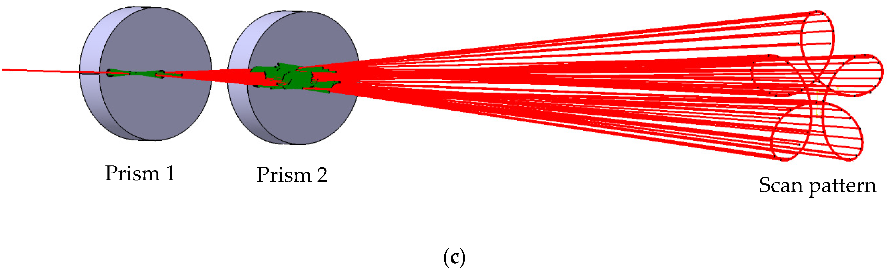
2. Scanners with Pairs of Rotational Risley Prisms

The principle scheme of a laser scanner with a pair of rotational Risley prisms is presented in Figure 1a.

Figure 1 shows the principle of the modelling process of the rotation of prisms performed using CATIA V5R20 and how this allows for the simulation of the scanning process, i.e., of the refraction of a laser beam (considered reduced to a single central ray) through the prism system. A simplifying hypothesis (and characteristic) of this entire study is that we perform it within the boundaries of geometrical optics. Thus, all the (Gaussian) laser beams are considered reduced to their central rays, and the dependence of the refractive indexes of the prisms materials with the laser wavelengths are not considered. As pointed out in the Introduction, there are studies focused on dispersion issues that occur especially when optical prisms are utilized, instead of wedges [15].

Figure 1b,c show the results of the simulation, with two ray bundles, generated for the two prisms rotating in the same direction (Figure 1b) and in opposite directions (Figure 1c), respectively. The ray bundles are intersected with a plane (the screen in Figure 1a) situated at a certain distance from the scanner. The scan patterns thus obtained are shown in dotted lines at the end of the light bundles. This simple procedure is utilized further on in Section 4 to obtain different shapes of the scan patterns.

The characteristic parameters of the system are (Figure 2): θ₁ and θ₂, the angles of the prisms; n₁ and n₂, the refractive indexes of the materials of Prism 1 and 2, respectively (indexes that are considered constant, as we do not take into account dispersion in the present work, as pointed out above); ω₁ and ω₂, the rotational speeds of the prisms; e, the distance between the two prisms (measured between the diopters perpendicular on the symmetry/optical axis (O.A.) of the components of the system); and L, the distance from the (final diopter perpendicular on the O.A. of the) scanner to the screen. The analysis of such scanners should also be based on Marshall’s synthetic and elegant parameters: k, the ratio of the angles of the prisms (initially defined in [4] in a more particular way, as ratio of the deviation angles D = (n−1) θ of each prism, obtained using the small angles approximation); and M, the ratio of the rotational speeds [4]:

$$k={\theta }_2/{\theta }_1 \mathrm{and} M={\omega }_2/{\omega }_1.$$

(1)

In Figure 1b,c, the two ray bundles were obtained for a certain modulus of M, but (b) for M > 0 (when the two prisms rotate in the same direction), and (c) for M < 0 (when the two prisms rotate in opposite directions). As a color convention in all such figures in the paper, bundles and patterns obtained for M > 0 are drawn in blue, while those obtained for M < 0 are drawn in red.

Four possible combinations of the relative positions of the two prisms can be obtained by considering all different possible orientations of the prism diopters [6]. By denoting with ‘a’ a diopter perpendicular on the O.A. and with ‘b’ a tilted one, these configurations are as follows (Figure 2): (a) ab-ab; (b) ab-ba; (c) ba-ba; and (d) ba-ab.

The extreme positions of the two rotational prisms are considered in Figure 2, namely for a relative rotational angle φ between the two prisms equal to 0 (on column 1) and equal to π (on column 2), respectively. The trajectories of the laser beam (considered reduced to its center ray) are pointed out in Figure 2 for each scanner configuration. From Snell’s refraction law, as well as from simple geometric considerations, the prism equations for each of the four scanner configurations (considering the two relative positions of the prisms in Figure 2) are provided in

Table 1. Equations of the four possible configurations of scanners with a pair of rotational Risley prisms (Figure 2)—for the cases of the maximum (1) and minimum (2) angular deviations.

Configuration (Figure 2)	(a) Scanner ab-ab	(b) Scanner ab-ba	(c) Scanner ba-ba	(d) Scanner ba-ab
Incidence angle	${\epsilon }_1=0$		${\epsilon }_1=-{\theta }_1$
Point I1	${\epsilon }_1’={\epsilon }_1$		$sin{\epsilon }_1=n_{1}sin{\epsilon }_1’$
Prism 1	${\epsilon }_2={\theta }_1$		$-{\epsilon }_1’+{\epsilon }_2={\theta }_1$
Point I2	$n_{1}sin{\epsilon }_2=sin{\epsilon }_2’$
Inter-prisms	${\epsilon }_2’-{\epsilon }_3={\theta }_1$	${\epsilon }_2’-{\epsilon }_3={\theta }_1\pm {\theta }_2$	${\epsilon }_2’-{\epsilon }_3=\pm {\theta }_2$	${\epsilon }_2’={\epsilon }_3$
Point I3	$sin{\epsilon }_3=n_{2}sin{\epsilon }_3’$
Prism 2	$\mp {\epsilon }_3’\pm {\epsilon }_4={\theta }_2$		$-{\epsilon }_3’+{\epsilon }_4=\pm {\theta }_2$
Point I4	$n_{2}sin{\epsilon }_4=sin{\epsilon }_4’$
Deviation angles $D_j^{max,min}$, j = a, b, c, d	$D_a^{max,min}={\epsilon }_4’\mp {\theta }_2$	$D_b^{max,min}={\epsilon }_4’$	$D_c^{max,min}={\epsilon }_4’$	$D_d^{max,min}={\epsilon }_4’\mp {\theta }_2$

Remark: The first sign in each of these expressions refers to the case of the maximum deviation $D_j^{max}$, j = a, b, c, d (for φ = 0), and the second sign refers to the case of the minimum deviation $D_j^{min}$, j = a, b, c, d (for φ = π).

. They are necessary to proceed to simulations, but also to deduce and analyze angular and linear deviations of the beam through the system. As a necessary remark, these equations can be utilized in simulations to trace the rays through the prism system—by ‘rotating’ each prism using the mechanical design program into different positions. However, they do not provide analytically the directions of the emerging rays to generate the scan patterns. For the latter, the (rather) complex mathematical approaches pointed out in the Introduction, for example [5,6,7], must be considered.

The minimum and maximum deviation angles $D_j^{max,min}$, j = a, b, c, d can be easily deduced by combining (on each of the four columns in Table 1) the equations of each scanner configuration.

From Figure 2a, for scanner (a) ab-ab

$$D_a^{max,min}=\mathit{arcsin}\left\{n_2\mathit{sin}\left[\pm {\theta }_2+\mathit{arcsin}\frac{\mathit{sin}\left[\mathit{arcsin}\left(n_{1}sin{\theta }_1\right)-{\theta }_1\right]}{n_2}\right]\right\}\mp {\theta }_2.$$

(2)

From Figure 2b, for scanner (b) ab-ba

$$D_b^{max,min}=\mathit{arcsin}\left\{n_2\mathit{sin}\left[\pm {\theta }_2+\mathit{arcsin}\frac{\mathit{sin}\left[\mathit{arcsin}\left(n_{1}sin{\theta }_1\right)-\left({\theta }_1\pm {\theta }_2\right)\right]}{n_2}\right]\right\}.$$

(3)

From Figure 2c, for scanner (c) ba-ba

$$D_c^{max,min}=\mathit{arcsin}\left\{n_2\mathit{sin}\left[\pm {\theta }_2+\mathit{arcsin}\frac{\mathit{sin}\left\{\mathit{arcsin}\left[n_1\mathit{sin}\left({\theta }_1-\mathit{arcsin}\frac{sin{\theta }_1}{n_1}\right)\right]\mp {\theta }_2\right\}}{n_2}\right]\right\}.$$

(4)

From Figure 2d, for scanner (d) ba-ab

$$D_d^{max,min}=\mathit{arcsin}\left\{n_2\mathit{sin}\left[\pm {\theta }_2+\mathit{arcsin}\left(\frac{n_1}{n_2}\mathit{sin}\left({\theta }_1-\mathit{arcsin}\frac{sin{\theta }_1}{n_1}\right)\right)\right]\right\}\mp {\theta }_2.$$

(5)

By considering the first order/Gaussian approximation, from Equations (2)–(5) the approximate (linearized) deviation angles have, for all four configurations, the following general (and well-known) equation:

$$D_{lin}^{max, min}=\left(n_1-1\right){\theta }_1\pm \left(n_2-1\right){\theta }_2.$$

(6)

Therefore, for the particular case of identical wedges, when $n_1=n_2=n$ and ${\theta }_1={\theta }_2=\theta$,

$$D_{lin}^{max}=2\left(n-1\right)\theta \mathrm{and} D_{lin}^{min}=0.$$

(7)

3. Linear Deviations of the Four Scanner Configurations

From Figure 2, for each of the four scanner configurations, the maximum and minimum linear deviations can be obtained, corresponding to the respective angular deviations deduced above for the $\phi =0$ and for the $\phi =\pi$ case, respectively. Both these maximum and minimum linear deviations consist of two components, one within the prism system, $y_P$, and the other one from the scanner to the screen, $y_S$, as shown for example in Figure 2(a1), but specific for each of the four configurations, (a) to (d):

$$y_j^{max,min}=y_{jP}^{max,min}+y_{jS}^{max,min}, j=a, b, c, d.$$

(8)

From the minimum deviations, $y_{jP}^{min}$, one obtains, for identical prisms, with $n_1=n_2=n$ and ${\theta }_1={\theta }_2=\theta$ (therefore for k = 1), the radius ${\Delta }_j, j=a, b, c, d$ of the blind spot, i.e., of the central disk of the scan patterns (Figure 2(a2,b2,c2,d2)). These blind spots are confirmed further on for the k = 1 cases of the scan patterns in Section 4 and are analyzed in Section 5. For the small angle approximation, simplified (i.e., linearized) expressions of these blind spot radiuses, ${\Delta }_j^{lin}, j=a, b, c, d$, can be obtained.

All the maximum deviations, $y_{jP}^{max}$, have for the particular case above (with identical prisms and the small angles approximation) the simple expression $2\left(n-1\right)L$. However, this approximate expression can be utilized only if the distance L is very large, for example in the order of km, as in satellite positioning, in Security and Defense, or in Remote Sensing. In contrast, for biomedical imaging, for example, but also for other scanning applications that utilize close range scanning, the exact expressions that are developed in the following should be employed.

The discussions are carried out further on in this section using the above procedure for each of the four scanner configuration, for the maximum deviations—column (1) in Figure 2, as well as for the minimum deviations—column (2) in Figure 2.

3.1. Linear Deviations of the Scanner (a) ab-ab

(1) Using Figure 2(a1), from Appendix A.1, with Equations (A1) and (A5), the maximum linear deviation in the prisms system (obtained for the $\phi =0$ case) is

$$y_{aP}^{max}=\frac{\left(e-b·\mathit{tan}{\theta }_1\right)·\mathit{tan}{\epsilon }_3+b·\mathit{tan}{\theta }_2·\mathit{tan}{\epsilon }_3’}{1-\mathit{tan}{\theta }_2·\mathit{tan}{\epsilon }_3’},$$

(9)

where the angles ${\epsilon }_3$ and ${\epsilon }_3’$ are given by Equation (A6).

From Figure 2(a1), the maximum linear deviation from the second diopter perpendicular on the O.A. to the screen (also for the $\phi =0$ case) is

$$y_{aS}^{max}=\left(L-I_{3}Q\right)·\mathit{tan}{D}_a^{max},$$

(10)

therefore, using Equation (A3),

$$y_{aS}^{max}=\left[L-\frac{\left[b-\left(e-b·tan{\theta }_1\right)·\mathit{tan}{\epsilon }_3\right]·tan{\theta }_2}{1-tan{\theta }_2·tan{\epsilon }_3’}\right]·\mathit{tan}{D}_a^{max},$$

(11)

where the angular deviation $D_a^{max}$ is given by Equation (2).

(2) Using Figure 2(a2), from Appendix A.2, with Equations (A2) and (A10), the minimum linear deviation (obtained for the $\phi =\mathsf{\pi }$ case) is

$$y_{aP}^{min}=\frac{\left(e-b·tan{\theta }_1\right)·\mathit{tan}{\epsilon }_3+b·tan{\theta }_2·tan{\epsilon }_3’}{1+tan{\theta }_2·tan{\epsilon }_3’},$$

(12)

where the angles ${\epsilon }_3$ and ${\epsilon }_3’$ are given in this case by Equation (A6) as well.

From Figure 2(a2), the minimum linear deviation from the second diopter perpendicular on the O.A. to the screen (also for the $\phi =\mathsf{\pi }$ case) is

$$y_{aS}^{min}=\left(L-I_{3}Q’\right)·\mathit{tan}{D}_a^{min},$$

(13)

therefore, using Equation (A8) and with the same angles,

$$y_{aS}^{min}=\left[L-\frac{\left[b-\left(e-b·tan{\theta }_1\right)·\mathit{tan}{\epsilon }_3\right]·tan{\theta }_2}{1+tan{\theta }_2·tan{\epsilon }_3’}\right]·\mathit{tan}{D}_a^{min},$$

(14)

where the angular deviation $D_a^{min}$ is given by Equation (2).

For identical prisms, for which $n_1=n_2=n$ and ${\theta }_1={\theta }_2=\theta$ (therefore k = 1), the radius of the blind spot/the central disk of the scan patterns (Figure 2(b2)) only comprises the first segment in Equation (A7), which is the ${\mathrm{I}}_3\mathrm{B}$ segment given by Equation (A2). This radius of the blind spot is therefore, from Equation (12),

$${\Delta }_a=\left(e-b·tan\theta \right)\mathit{tan}{\epsilon }_3=\left(e-b·tan\theta \right)\frac{n·cos\theta -\sqrt{1-n^2·si{n}^2\theta }}{n·si{n}^2\theta +cos\theta ·\sqrt{1-n^2·si{n}^2\theta }}.$$

(15)

In the particular case of the small angles approximation, this expression becomes

$${\Delta }_a^{lin}=\left(e-b\theta \right)\frac{n-\sqrt{1-n^2·{\theta }^2}}{n·{\theta }^2+\sqrt{1-n^2·{\theta }^2}}$$

(16)

In all such equations, the boundary conditions, for example $1-n^2·si{n}^2\theta >0$ in Equation (15), are equivalent with the conditions to avoid total reflections on the second and fourth diopter of the prisms of the scanners in Figure 2—aspects to be discussed in Section 5.1.

3.2. Linear Deviations of the Scanner (b) ab-ba

(1) Using Figure 2(b1), from Appendix B.1, with Equation (A17), using Equations (A12) to (A14), the maximum linear deviation (obtained for the $\phi =0$ case) is

$$y_{bP}^{max}=\left[e-b\left(tan{\theta }_1+tan{\theta }_2\right)\right]·\frac{\mathit{sin}\left({\epsilon }_3+{\theta }_2\right)·\mathit{cos}\left({\epsilon }_4-{\theta }_2\right)}{cos{\epsilon }_3·cos{\epsilon }_4}+b·tan{\theta }_2·tan{\epsilon }_4,$$

(17)

where the angles ${\epsilon }_4$ and ${\epsilon }_3$ are given by Equation (A18).

From Figure 2(b1), the maximum linear deviation from the second diopter perpendicular on the O.A. to the screen (also for the $\phi =0$ case) is

$$y_{bS}^{max}=L·\mathit{tan}{D}_b^{max},$$

(18)

where the angular deviation $D_b^{max}$ is given by Equation (3).

(2) Using Figure 2(b2), from Appendix B.2, with Equation (A21), the minimum linear deviation (obtained for the $\phi =\pi$ case) is

$$y_{bP}^{min}=\left[e-b\left(tan{\theta }_1+tan{\theta }_2\right)\right]·\frac{\mathit{sin}\left({\epsilon }_3-{\theta }_2\right)·\mathit{cos}\left({\epsilon }_4+{\theta }_2\right)}{cos{\epsilon }_3·cos{\epsilon }_4}+b·tan{\theta }_2·tan{\epsilon }_4,$$

(19)

where the angles ${\epsilon }_3$ and ${\epsilon }_4$ are given in this case by Equation (A22).

From Figure 2(a2), the minimum linear deviation from the second diopter perpendicular on the O.A. to the screen (also for the $\phi =\pi$ case) is

$$y_{bS}^{min}=L·\mathit{tan}{D}_b^{min},$$

(20)

where the angular deviation $D_b^{min}$ is given by Equation (3).

As in Section 3.1, for identical prisms, the radius of the blind spot is the segment $I_{3}M’$ from Equation (A19) (Figure 2(b2)), from Equation (19),

$${\Delta }_b=\left(e·cos\theta -2b·sin\theta \right)\left(\frac{n·cos\theta }{\sqrt{1-n^2·si{n}^2\theta }}-1\right)·sin\theta .$$

(21)

In the particular case of the small angles approximation, this expression becomes

$${\Delta }_b^{lin}=\left(e-2b\theta \right)\left(n/\sqrt{1-n^2{\theta }^2}-1\right)\theta .$$

(22)

3.3. Linear Deviations of the Scanner (c) ba-ba

(1) Using Figure 2(c1), from Appendix C.1, with Equations (A24) and (A31), the maximum linear deviation (obtained for the $\phi =0$ case) is

$$y_{cP}^{max}=e\cdot tan{\epsilon }_4+b·tan{\theta }_1·tan{\epsilon }_2+\frac{tan{\epsilon }_2’-tan{\epsilon }_4}{1+tan{\theta }_2·tan{\epsilon }_2’}\left[e-b\left(1+tan{\theta }_1·tan{\epsilon }_2\right)tan{\theta }_2\right],$$

(23)

where the angles ${\epsilon }_2$, ${\epsilon }_2’$, and ${\epsilon }_4$ are given by Equation (A23).

From Figure 2(c2), the maximum linear deviation from the second diopter perpendicular on the O.A. to the screen (also for the $\phi =0$ case) is

$$y_{cS}^{max}=L·\mathit{tan}{D}_c^{max},$$

(24)

where the angular deviation $D_c^{max}$ is given by Equation (4).

(2) Using Figure 2(c2), from Appendix C.2, with Equations (A24) and (A38), the minimum linear deviation (obtained for the $\phi =\pi$ case) is

$$y_{cP}^{min}=e\cdot tan{\epsilon }_4+b·tan{\theta }_1·tan{\epsilon }_2+\frac{tan{\epsilon }_2’-tan{\epsilon }_4}{1+tan{\theta }_2·tan{\epsilon }_2’}\left[e-b\left(1-tan{\theta }_1·tan{\epsilon }_2\right)tan{\theta }_2\right],$$

(25)

where the angles ${\epsilon }_2$ and ${\epsilon }_2’$ are given by Equation (A23), while ${\epsilon }_4$ is given by Equation (A39).

From Figure 2(c2), the minimum linear deviation from the second diopter perpendicular on the O.A. to the screen (for the $\phi =\pi$ case) is

$$y_{cS}^{min}=L·\mathit{tan}{D}_c^{min},$$

(26)

where the angular deviation $D_c^{min}$ is given by Equation (4).

For identical prisms, the radius of the blind spot is, from Equation (25),

$${\Delta }_c=\frac{e-b\left(1-tan\theta ·tan{\epsilon }_2/tan{\epsilon }_2’\right)}{1+1/tan{\epsilon }_2’},$$

(27)

where the angles ${\epsilon }_2$ and ${\epsilon }_2’$ are given by Equation (A23) for the particular case of identical prisms (i.e., of $n_1=n_2=n$ and ${\theta }_1={\theta }_2=\theta$). In the particular case of the small angles approximations, Equation (27) becomes

$${\Delta }_c^{lin}=\left[ne-\left(n-1\right)b\right]/\left[1+\left(n-1\right)\theta \right].$$

(28)

3.4. Linear Deviations of the Scanner (d) ba-ab

(1) Using Figure 2(d1), from Appendix D.1, with Equations (A41), (A42), and (A45), the maximum linear deviation (obtained for the $\phi =0$ case) is

$$y_{dP}^{max}=\frac{\left(b·tan{\theta }_1\cdot tan{\epsilon }_2+e·tan{\epsilon }_2’\right)·cos{\theta }_2·cos{\epsilon }_3’+b·sin{\theta }_2·sin{\epsilon }_3’}{\mathit{cos}\left({\theta }_2+{\epsilon }_3’\right)},$$

(29)

where the angles ${\epsilon }_2$, ${\epsilon }_2^{’}$, and ${\epsilon }_3’$ are given by Equation (A46).

From Figure 2(d1), the maximum linear deviation from the second diopter perpendicular on the O.A. to the screen (for the $\phi =0$ case) is

$$y_{dS}^{max}=\left(L-I_{3}Q\right)·\mathit{tan}{D}_d^{max},$$

(30)

therefore, using Equation (A44),

$$y_{dS}^{max}=\left[L-\left[b\left(1+tan{\theta }_1\cdot tan{\epsilon }_2\right)+e·tan{\epsilon }_2’\right]·\frac{sin{\theta }_2·cos{\epsilon }_3’}{cos{\epsilon }_4}\right]·\mathit{tan}{D}_d^{max}.$$

(31)

where the angular deviation $D_d^{max}$ is given by Equation (5).

(2) Using Figure 2(d2), from Appendix D.2, with Equations (A41), (A42) and (A50), the minimum linear deviation (obtained for the $\phi =\pi$ case) is

$$y_{dP}^{min}=e\left[tan{\epsilon }_2’+\left(1-tan{\epsilon }_2’\right)\frac{sin{\theta }_2}{cos{\epsilon }_4}\right]+b·tan{\theta }_1\cdot tan{\epsilon }_2·\left(1-\frac{sin{\theta }_2}{cos{\epsilon }_4}\right),$$

(32)

where the angles ${\epsilon }_2^{’}$ and ${\epsilon }_3’$ are given by Equation (A46), and ${\epsilon }_4$ is given by Equation (A51).

From Figure 2(d2), the minimum linear deviation from the second diopter perpendicular on the O.A. to the screen (also for the $\phi =\pi$ case) is, with the same angles,

$$y_{dS}^{min}=\left(L-I_3{I}_4·cos{\epsilon }_3’\right)·\mathit{tan}{D}_d^{min},$$

(33)

therefore, using Equation (A48),

$$y_{dS}^{min}=\left[L+\left[b·tan{\theta }_1\cdot tan{\epsilon }_2-e\left(1-tan{\epsilon }_2’\right)\right]\frac{sin{\theta }_2·cos{\epsilon }_3’}{cos{\epsilon }_4}\right]·\mathit{tan}{D}_d^{min},$$

(34)

where the angular deviation $D_d^{min}$ is given by Equation (5).

For identical prisms, the radius of the blind spot is, from Equation (32),

$${\Delta }_d=b·tan \theta ·\mathit{tan}{\epsilon }_2+e·tan\left[\mathit{arcsin}\left(n·sin{\epsilon }_2\right)\right].$$

(35)

In the particular case of the small angles approximations, this expression becomes

$${\Delta }_d^{lin}=\left(n-1\right)\left(e-b\theta /n\right)\theta .$$

(36)

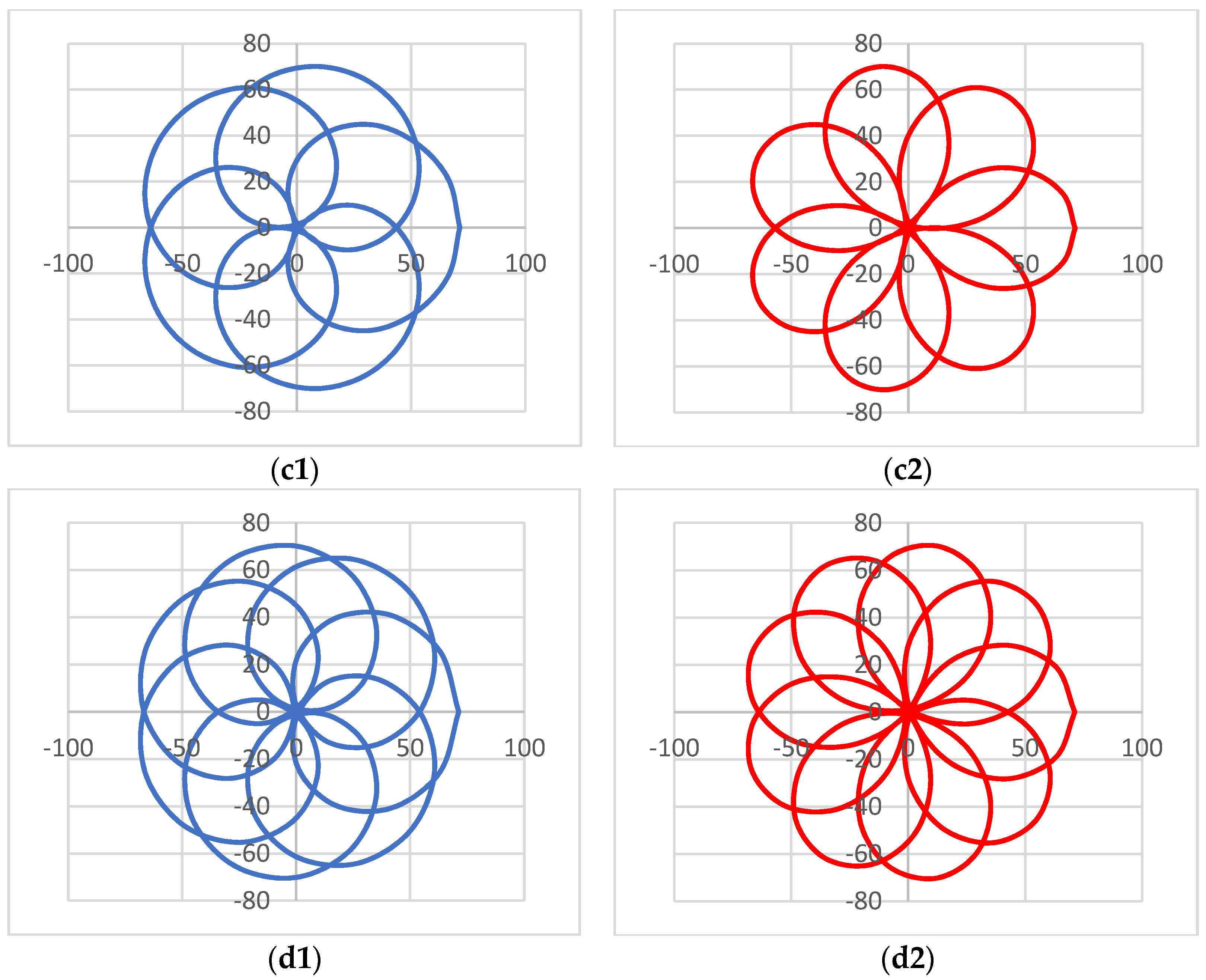
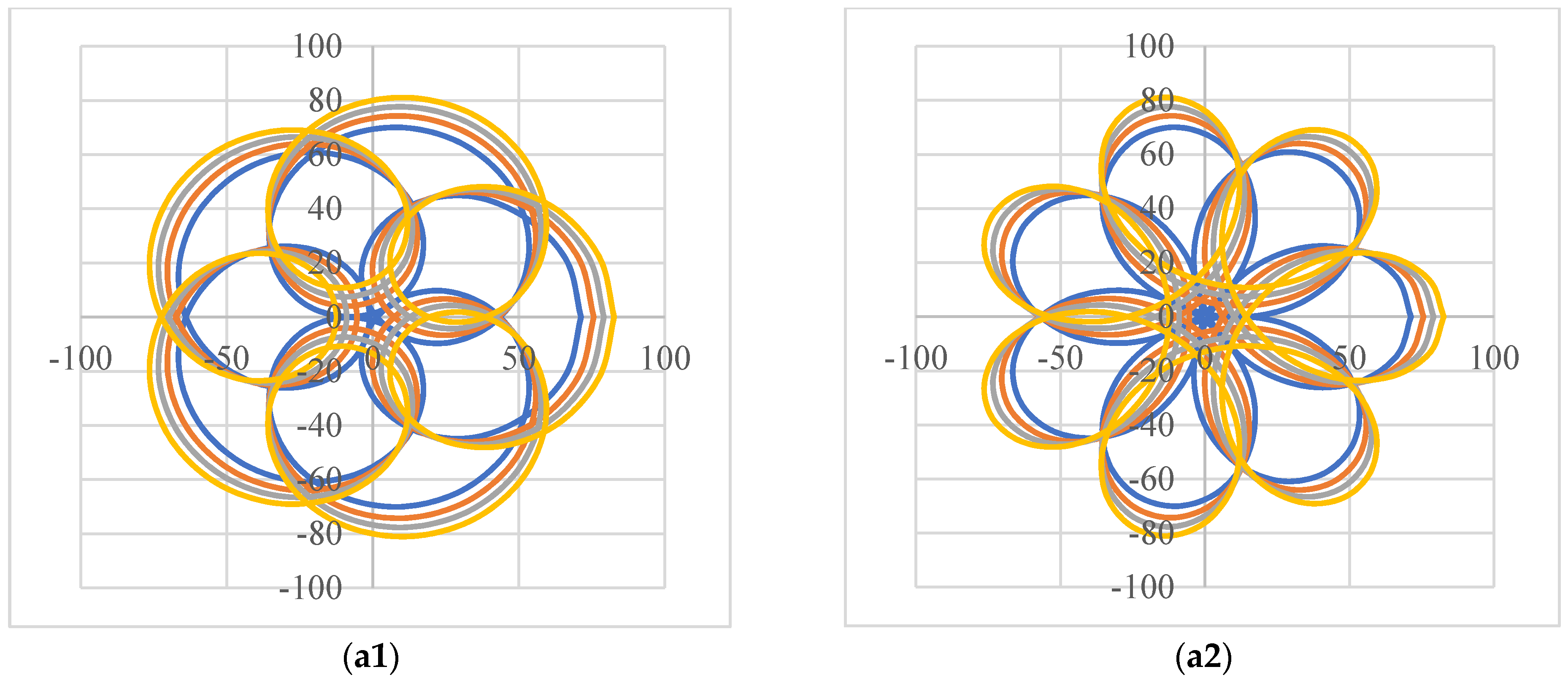
4. Results of Modeling and Simulations: Shapes of the Scan Patterns

Using a commercially-available mechanical design program, CATIA5V20, by considering finite rotations of the two prisms shown in Figure 1a, the ray bundles can be obtained, as demonstrated in Figure 1b,c. Therefore, by intersecting them with a certain plane (i.e., the screen positioned at the distance L from the final diopter perpendicular on the O.A.—Figure 2), the generated scan patterns can be obtained. In the following part of the study, mostly the case of the scanner configuration in Figure 2d is considered to carry out simulations, while a comparison of the scan patterns of all four configurations in Figure 2a–d is also provided.

To better understand the kinematics of the laser spot, in Figure 3 the case when one of the prisms is fixed and the other one is mobile is considered. Thus, for four different positions rotated with 90° of the fixed prism, the rotation of the other prism produces four circles in the scanned plane—one for each position of the fixed prism. Because of the different longitudinal position of the two prisms (i.e., along the O.A.), the circles obtained when Prism 1 is mobile and Prism 2 is fixed are larger, as Prism 1 is situated at a longer distance from the screen. By combining the two rotational movements of the prisms, a Rhononea-type curve is obtained, albeit with different equations than such classical curves [62], as shown initially in Figure 1 for the same |M|, but with an opposite (Figure 1c) versus an identical (Figure 1b) rotational sense.

Examples of such scan patterns, with a multi-parameter analysis carried out considering the M and k parameters in Equation (1), as well as the other constructive parameters of the scanners are provided in Figure 4, Figure 5, Figure 6, Figure 7 and Figure 8.

In Figure 4, the scan patterns are generated for the most common case of identical prisms, i.e., of k = 1 (obtained for D₁ = D₂ = 2°) and several values of M, positive on column 1 and negative on column 2: (a) |M| = 2; (b) |M| = 4; (c) |M| = 6; (d) |M| = 8. The |M| = 4 case corresponds to the constructions in Figure 1.

One can remark that the number of loops of a pattern is μ = M−1 for M > 0 (e.g., μ = 1 for M = 2, μ = 2 for M = 3, etc.). The difference between positive and negative values of M can be seen, as μ = |M|+1 for M < 0 (e.g., μ = 3 for M = 2, μ = 4 for M = 3, etc.). From this comparison, the number of loops is in general, as first observed in [4],

μ = |M − 1|,

(37)

Another relevant, simple equation can be extracted from this discussion regarding the number of loops of a scan pattern, obtained for the same |M|:

μ(M < 0) = μ(M > 0) + 2.

(38)

One can also observe (easier for smaller |M|), as a specificity of these Risley prism curves, the way inward loops are generated for M > 0, while outward loops are generated for M < 0.

In Figure 5, scan patterns obtained for |M| = 6 are shown, for increasing values of k: from (a) k = 2/4 = 1/2 (obtained for D₁ = 4° and D₂ = 2°) to (b) k = 4/2 = 2 (for D₁ = 2° and D₂ = 4°), (c) k = 6/2 = 3 (for D₁ = 2° and D₂ = 6°), and (d) k = 10/2 = 5 (for D₁ = 2° and D₂ = 10°). The intermediate k = 2/2 = 1 case for this |M| was already shown in Figure 4c. As a remark, these specific values have been chosen because such Risley prisms are commercially available, for example from Thorlabs [63].

From Figure 5, by making a comparison along each of the two columns, one can see that as k increases, the loops intersect more and more. This is due to the variation of the minimum angular deviation that can be obtained as θ₂ increases—in the case of the scanner configuration in Figure 2d—from Equation (5). This discussion is made in detail in Section 6.

Figure 6 shows the differences between the scan patterns, for four possible values of the distance e between the two identical Risley prisms, and for M = 6 (column 1) and M = −6 (column 2). These values of e are different for each pair of prisms, considering their (individual) deviation angles: (a) D = 2°, (b) D = 4°, and (c) D = 6°. The D = 10° case is not shown here anymore, as it is similar to the latter, but the obtained values are analyzed in Section 6 for such a case as well.

Specifically, the two values of e are considered starting from a small one which (barely) avoids the situation when the prisms would touch, up to a maximum value e_max specific to each D. For the latter the condition to still have the refractions inside the prisms for their 2b diameter was considered for each pair of prisms. The ascertainment of these values e_max was done purely graphically, using the mechanical design program (as an example of the utility of this fast-to-operate method).

Figure 7 presents a study of the scan patterns when varying significantly the values of the distance L from the scanner to the screen. Thus, a 10-times increase was considered for L from one pattern to another, i.e., from L = 10 to 100 m. The L = 1 m case was already considered in Figure 4c. These examples refer to scan patterns obtained for M = 6 and k = 1. This confirms the remark made at the beginning of Section 3: the maximum linear deviation (i.e., the radius of the FOV) can be considered proportional with the distance L if this distance is large enough, so that the linear deviations inside the prisms system can be neglected.

To conclude this presentation, in Figure 8 the differences between the scan patterns of the four scanner configurations in Figure 2 are shown. The case of |M| = 8 and of k = 1 (obtained this time for D₁ = D₂ = 10°) was considered. The large angle prisms were considered as an example to better distinguish between the scan patterns. The order of the patterns with regard to their size/outer radius/FOV is, in all graphs of Figure 8, from the smallest to the largest: (c), (b), (d), and (a).

The scan patterns are discussed further on from the point of view of their dimensions in Section 6, in a multi-parameter analysis carried out in relationship with the one referring to the angular and linear deviations in Section 5.

5. Multi-Parameter Analysis of Angular and Linear Deviations

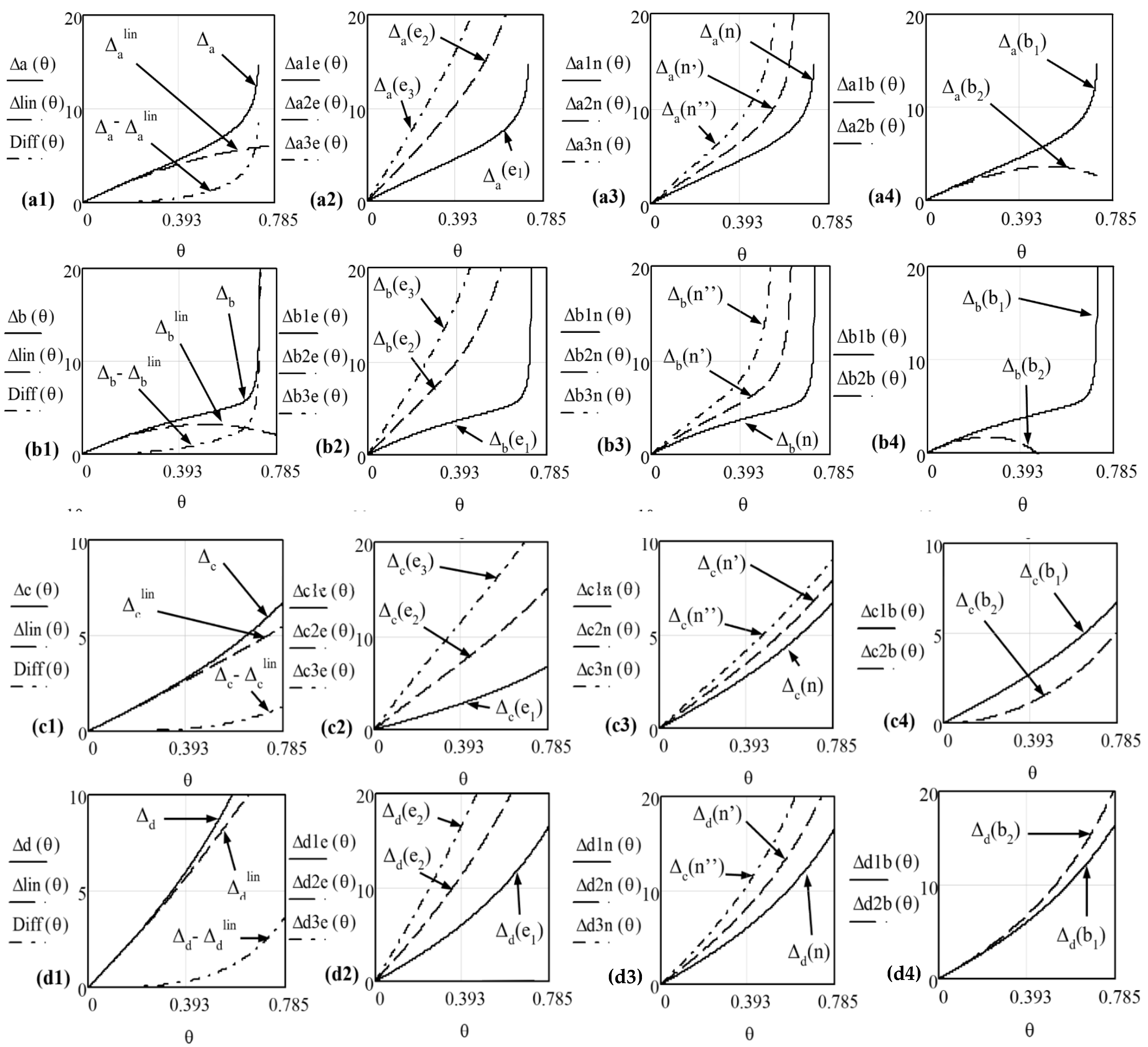
5.1. Multi-Parameter Analysis of Angular Deviations

The first step of the analysis refers to the angular deviations of the four scanners configurations presented in Figure 2, with expressions given by Equations (2) to (5).

Figure 9a shows the maximum angular deviations $D_j^{max}$, j = a, b, c, d as functions of the angle of the prisms—for the case of identical prisms, therefore with $n_1=n_2=n$ and ${\theta }_1={\theta }_2=\theta$ (i.e., with k = 1). These exact values of deviations are compared with the approximate/linearized one, $D_{lin}^{max}$, given by Equation (7). One can remark that the latter is the same regardless of the scanner configuration. Figure 9b provides the error between the case when the maximum angular deviations are considered in their linear approximation, instead of their exact values. One can see that this approximation can be roughly valid up to a prism angle of 0.087 rad = 10°, and therefore for optical wedges. For prisms with a larger angle, one must consider the exact expressions of the deviations—angular as well as linear.

Another conclusion that can be extracted from the study in Figure 9b is that, from Figure 2, the configurations (a) and (d) have much higher non-linearities than configurations (b) and (c). The strongest non-linearity refers to configuration (a), while the weakest one characterizes configuration (c).

From Figure 9 one can see that a limit prism angle, ${\theta }_j^{lim}$, j = a, b, c, d, can be determined for each scanner configuration, as a function of the refractive index n of the prisms, as remarked from Figure 10 as well.

From Figure 2a this limit prism angle is obtained from the conditions to avoid total reflections on the second and fourth diopter of the scanner. These conditions are

$$\epsilon {’}_2<\pi /2 \mathrm{and} \epsilon {’}_4<\pi /2, \mathrm{respectively}.$$

(39)

By using each scanner equation in Table 1, these inequations can give limit values of the angles of each prism, ${\theta }_1$ and ${\theta }_2$. For the particular case of identical prisms and using the small angles approximation, these inequations can then provide an approximate limit value of ${\theta }_j^{lim}$, j = a, b, c, d. It is important to remark from Figure 9 and Figure 10 that such limits are higher than the exact ones, which are smaller when the Gaussian approximation is not utilized. Using for the limit angles of each prism, the notations are

$${\epsilon }_{1l}=\mathit{arcsin}1/n_1 \mathrm{and} {\epsilon }_{2l}=\mathit{arcsin}1/n_2,$$

(40)

respectively, and by applying the above procedure for each scanner, one has the following:

-

From Figure 2a, for scanner (a) ab-ab, the conditions to have a beam emerging from the scanner are

$${\theta }_1<{\epsilon }_{1l} \mathrm{and} {\theta }_2<{\epsilon }_{2l}-\mathit{arcsin}\frac{\mathit{sin}\left[\mathit{arcsin}\left(n_{1}sin{\theta }_1\right)-{\theta }_1\right]}{n_2},$$

(41)

from which, for identical prisms and for small angles,

$$\theta <n/\left(n-1+\sqrt{n^2-1}\right)={\theta }_a^{lim}.$$

(42)

-

From Figure 2b, for scanner (b) ab-ba, the conditions to have a beam emerging from the scanner are

$${\theta }_1<{\epsilon }_{1l} \mathrm{and} n_{2}sin({\theta }_2-{\epsilon }_{2l})-{\theta }_2<{\theta }_1-\mathit{arcsin}\left(n_{1}sin{\theta }_1\right),$$

(43)

from which, for identical prisms and for small angles,

$$\theta <n/2\left(n-1\right)={\theta }_b^{lim}.$$

(44)

-

From Figure 2c, for scanner (c) ba-ba, the conditions to have a beam emerging from the scanner are

$${\theta }_1-\mathit{arcsin}\frac{sin{\theta }_1}{n_1}<{\epsilon }_{1l} \mathrm{and} n_2\mathit{sin}\left({\epsilon }_{2l}-{\theta }_2\right)>sin\left\{\mathit{arcsin}\left[{\theta }_1-\mathit{arcsin}\frac{sin{\theta }_1}{n_1}\right]-{\theta }_2\right\},$$

(45)

from which, for identical prisms and for small angles, the condition (44) is valid in this case, as well, therefore ${\theta }_c^{lim}={\theta }_b^{lim}$. However, this is clearly not true for the exact limit angles that refer to the non-linear curves of the maximum angular deviations in Figure 9a.

-

From Figure 2d, for scanner (d) ba-ab, the conditions to have a beam emerging from the scanner are

$${\theta }_1-\mathit{arcsin}\frac{sin{\theta }_1}{n_1}<{\epsilon }_{1l} \mathrm{and} n_2\mathit{sin}\left({\epsilon }_{2l}-{\theta }_2\right)>n_1\mathit{sin}{\theta }_1-\mathit{arcsin}\frac{sin{\theta }_1}{n_1},$$

(46)

from which, for identical prisms and for small angles,

$$\theta <n/\left(2n-1\right)={\theta }_d^{lim}.$$

(47)

While the stress in this analysis was put on the variation of angular deviations, another approach, entirely focused on the limit angles of Risley prisms, was done in [50].

The parameter the deviations depend upon is the refractive index of the prisms. Therefore, the second part of this study of maximum angular deviations is presented in Figure 10, where the angles $D_j^{max}$, j = a, b, c, d are shown as functions of the angle of the prism ${\theta }_1={\theta }_2=\theta$, as well, but for two values of the refractive index of the two prisms (when $n_1=n_2$): for $n=1.517$ (as in Figure 9) and for $n’=1.7$. One can see that the maximum angular deviation, therefore the FOV, is slightly increased when using Risley prisms with a higher refractive index, although the angle prism limit ${\theta }_d^{lim}$ that can be chosen is smaller for a higher n. The latter aspect is in good agreement with Equation (47).

Values determined graphically for the limit angles, for both considered refractive indexes, are extracted from Figure 10 in

Table 2. Limit prism angle ${\theta }_j^{lin}\left(rad\right), j=a, b, c, d$ with regard to refractive index (the identical prisms case, i.e., k = 1).

Scanner Configurations	Refractive Index
	n = 1.517	n’ = 1.7
Figure 2a	${\theta }_a^{lim}\left(n\right)=0.523=\pi /6$	${\theta }_a^{lim}\left(n’\right)\cong 0.43$
Figure 2b	${\theta }_b^{lim}\left(n\right)=0.72$	${\theta }_b^{lim}\left(n’\right)\cong 0.6$
Figure 2c	${\theta }_c^{lim}\left(n\right)=0.96$	${\theta }_c^{lim}\left(n’\right)\cong 0.785=\pi /4$
Figure 2d	${\theta }_d^{lim}\left(n\right)=0.53$	${\theta }_d^{lim}\left(n’\right)\cong 0.45\cong \pi /7$

Remark: One must highlight that these (exact) limit angles must be used in general, while the approximate values obtained in Equation (42), (44), and (47) are restricted to the small angle domain (i.e., for $\theta$ < 10°).

.

5.2. Multi-Parameter Analysis of Linear Deviations

Figure 11 shows a study of the minimum linear deviations/radiuses ${\Delta }_j\left(\theta \right), j=a, b, c, d$ of the blind spot, i.e., of the central disk of the scan patterns. As discussed in Section 3, these radiuses refer to the case of two identical prisms (with $n_1=n_2=n$ and ${\theta }_1={\theta }_2=\theta$, therefore k=1), when emergent beams are in this case parallel to the O.A., as marked with dotted lines in Figure 2(a2,b2,c2,d2). For the four scanner configurations (Figure 2), these radiuses are given by: (a) Equation (15), (b) Equation (21), (c) Equation (27), and (d) Equation (35).

The characteristic parameters of this study are the prism angles $\theta$, the distance e between them, their refractive index n, and the radius b of each circular prism. In each of the four steps of the following analysis, three of these parameters were kept constant, while the other ones were considered with two or three values to determine the variance of the ${\Delta }_j\left(\theta \right), j=a, b, c, d$ functions. A maximum limit of 45° for the prism angle $\theta$ was considered, although considering a value of around 18°9’ ≈ 0.314 rad for the optical wedge angle (to produce an individual prism deviation D equal to 10°) [60] is also useful when referring to the most utilized devices. Considering Figure 11, on its columns are the following:

(1) Exact radiuses ${\Delta }_j\left(\theta \right), j=a, b, c, d$ and approximate/linearized ones ${\Delta }_j^{lin}\left(\theta \right), j=a, b, c, d$, the latter given by (a) Equation (16), (b) Equation (22), (c) Equation (28), and (d) Equation (36) were determined for the most common parameters n = 1.517, e = 25 mm, and b = 12.7 mm (the latter corresponding to commercially-available prisms of 1” in diameter [60]). The difference $({\Delta }_j-{\Delta }_j^{lin})\left(\theta \right)$ between these exact and approximate radiuses for each scanner was also determined. One can see the differences between the four configurations, with configuration (b) providing the smallest values of Δ, and configuration (d) the largest ones. From the point of view of the linearity, the approximation ${\Delta }_j^{lin}$ works up to D = 10°, and even up to θ = π/8. The limit angles calculated in Equations (40)–(47) apply here as well.

(2) Exact radiuses ${\Delta }_j\left(\theta \right), j=a, b, c, d$ were studied for three values of the distance between the prisms e₁ = 25, e₂ = 50, and e₃ = 75 mm (with n = 1.517 and b = 12.7 mm), with the remark that much larger values of e can be considered, as studied in Figure 6. The same interval (of up to 20 mm) was set here for Δ, and the same conclusion can be reached for the smallest value of e. For the two larger e, Δ gets closer for the four configurations, (a) to (d); therefore, if one aims to minimize Δ, going for the smallest possible e is the solution. As a remark, the (minimum) value e equal to 25 mm was chosen to avoid the situation when the prisms were getting in contact even for commercially-available prisms with the maximum common deviation D = 10°, for a 1” diameter of the prisms. To increase Δ, increasing e is the best solution for all configurations.

(3) Exact radiuses were obtained for three values of the refractive index of the prisms, n = 1.517, n’ = 1.7, and n” = 1.9 mm (for e = 25 mm and b = 12.7 mm). For all configurations, Δ increases with n, but this is a less effective solution. A useful remark is that a minimum Δ is obtained for the first, most common n (corresponding to the BK7 optical glass).

(4) Exact radiuses were studied for two values of the radius of the circular prisms, b₁ = 12.7 and b₂ = 25.4 mm (with n = 1.517 and e = 25 mm). For the smaller b, Δ is slightly higher for configurations (a) and (b), higher for configuration (c), and lower for configuration (d). However, to be cost-effective, one must consider that prisms with b = 12.7 mm (i.e., with 1” in diameter) are commercially-available and therefore less costly.

6. Analysis of Scan Patterns Dimensions: Rules-of-Thumb for Scanner Designs

A necessary correlation must be made between the scan patterns analyzed in Section 4 and the angular and linear deviations analyzed in Section 5. This allows for the multi-parameter analysis of the dimensions of the scan patterns, to complete the multi-parameter analysis of their shapes, performed on examples in Section 4. These two types of (correlated) analyses allow one to extract rules-of-thumb for the design of Risley prism scanners to satisfy the requirements of certain applications.

6.1. FOV of Scanners with a Pair of Rotational Risley Prisms

6.1.1. Study with Regard to the Prisms Angles

One of the most common requirement of applications is to have the largest possible FOV. From Figure 9 one can see that the optimal choice of prism orientation in order to reach this maximum FOV is in the (a) configuration in Figure 2, followed by the (d) configuration. In contrast, configurations (b) and (c) produce, using the same pair of (identical) prisms, a much smaller maximum angular deviation. The same inequality

$$D_a^{max}>D_d^{max}>D_b^{max}>D_c^{max},\forall \theta$$

(48)

can be observed from the simulated scan patterns analysis in Figure 8. However, what cannot be entirely obtained from simulations is the limit of the prism angle for which the inequality (48) still holds. Thus, from Figure 9a one can see that this limit angle is π/8 rad. This makes the above conclusion valid for optical wedges, which have prism angles smaller than (roughly) π/18 rad (the deviation of a single prism is D = 10° for θ = 18°9′ for n = 1.517).

As θ = π/8 rad is the limit angle for Risley prisms scanners in the (a) and (d) configurations, from Figure 9, if one aims to reach higher maximum deviation angles and therefore a larger FOV, the (b) configuration could be used up to prism angles of θ ≈ 0.72 rad, or the (c) configuration for up to θ ≈ 0.96 rad (both values evaluated for n = 1.517).

From the point of view of these limit prism angles, one should consider the analysis in Section 5.1, based on the condition to avoid the total reflection on the second diopter of each prism, and therefore Equation (41) for (a), Equation (43) for (b), Equation (45) for (c), and Equation (46) for (d).

One could also consider a k ≠ 1 case, therefore using different prisms, in order to increase the FOV. Such an approach would give results that are in-between the above cases of (a) to (d) configurations (with identical prisms), in a more complicated analysis that could be subject of a future optimization but may be too complicated to be of interest in practice. Therefore, one may consider a (simpler) scanner with identical prisms without failing in an optimization process from the point of view of the FOV. The maximum angular deviations, namely Equations (2)–(5), as well as the linear ones, namely Equation (6), give the maximum FOV of the scan pattern for each configuration. From Figure 4 this radius is identical for different values of M and from Figure 5 it increases with k, in agreement with Equation (5) for configuration (d).

As concluded in the previous section, one must also point out that, from Figure 9, configurations (a) and (d) have the strongest non-linearities of the deviation versus prism angle function, while configurations (b) and (c) have the lowest. One could use this conclusion to build scanners with prism angles close to the values in Table 2, for example (for a specific n), to maximize the angular deviation and therefore the FOV.

6.1.2. Study with Regard to the Refractive Index n of the Prisms

From Figure 10, by choosing a higher value for n (for both prisms, as the k = 1 case was also considered here for simplicity), the same maximum deviation angle, and therefore the same FOV can be reached, for a smaller prisms angle θ, although the non-linearity of the $D_j^{max}$ curve is roughly the same. In the small angles domain, though, there is a clear gain from choosing a higher n, as $D_{lin}^{max}$ is higher, both from the graphs in Figure 10 and from Equation (7).

6.1.3. Study with Regard to the Distance e between the Two Prisms

From Figure 6, the most significant gain with regard to e from the point of view of the FOV is for prisms with D = 2° and less for D = 4°, while for D = 6° or 10° (the latter not represented in Figure 6 as the latter two cases are too similar), this gain becomes less important. In conclusion, one should go for an increase of e only for small angle optical wedges, especially with D = 2° (for which θ = 3°53′ for n = 1.517). The relevant aspect is that for such a system e can be increased a lot (i.e., up to 350 mm in Figure 6a), although one must also consider a trade-off between the gain in FOV and the dimensions of the system. A folding of such a large distance e could be considered in this case, using supplemental mirrors, as for other types of scanners [64].

6.1.4. Study with Regard to the Distance L from the Scanner to the Target

The solution to increase FOV by increasing L may be applicable only in some situations, as in general the magnitude of L is imposed by the application itself. For Remote Sensing or for detection in Security and Defense, for example, L is large, and the simple $2L{D}_{lin}^{max}$ relationship can be applied for the radius of the FOV, neglecting the small terms of $y_{jP}^{max},j=a,b,c,d$ deduced in Section 3 (Figure 7). For other applications, such as endoscopy (but also for more common setups, with 1” diameter prisms), L can be comparable to the diameter of the prisms, 2b, and the dimensions of the FOV must be calculated taking into account the exact values of the maximum linear deviations (Equation (8)).

An interesting case is represented by applications that have intermediate values of L, of up to (or around) 1 m, as considered in all the studies in Figure 4, Figure 5 and Figure 6, as well as in Figure 8, Figure 9 and Figure 10. For such situations (in optical metrology, laser manufacturing, 3D printing, etc.) and especially when the distance from the scanner to the target plane is kept constant, L can be increased (as pointed out for the dimension e above) without increasing the dimensions of the system by using three or even only two supplementary mirrors [64]. Thus, a supplemental increase of the FOV can be obtained.

6.1.5. Study with Regard to the Scanner Configuration

From the scan patterns of the four scanner configurations presented in Figure 8 (for |M| = 8 and D₁ = D₂ = 10°), the size/FOV of these patterns is larger for configuration (a) than for (d), (b), and (c). This corresponds exactly to (and comes from) the order of the maximum angular deviations from the analysis in Figure 9 (see Equation (48)). In addition, one can see that the patterns are close, two by two, on the one hand for configurations (a) with (d), and on the other hand for configurations (b) with (c), as highlighted in Figure 9a as well.

6.2. Blind (Inner) Zone of the Scan Patterns

This aspect of the central blind spot is particularly important in practice, for applications such as laser processing. There are two methods to produce a blind spot in the center of the FOV. The first and most reliable one implies using identical Risley prisms, as the expressions of the ${\Delta }_j, j=a, b, c, d$ radiuses deduced in Section 3 are not functions of the distance L to the target, as can also be observed from Figure 4. This is important in applications where this distance L is variable and cannot be controlled (imaging, for biomedical or industrial purposes, Remote Sensing, CAD/CAM with laser scanners, etc.).

From the study related to Figure 11 in Section 5.2, the ${\Delta }_j, j=a, b, c, d$ radiuses can be decreased by decreasing e, n, and b, the latter excepting configuration (d). One can also see from Figure 11, column (1), that configuration (b) provides the smallest values of Δ, then (in this order) configurations (a), (c), and (d). Thus, depending on the application, one can chose between one or the other configuration, for example (b) for laser manufacturing of contact lenses and (d) for scanning the entire FOV in biomedical apparatuses or machine vision.

A second way of tackling the inner blind zone is by considering different k ≠ 1 cases. For k = 2, 3, and 5 in Figure 5b–d, the minimum linear deviation given, according to Equation (8), by the sum of Equations (29) and (31), becomes negative, as the tip of the loops ‘passes’ beyond the O.A. A disc untouched by the laser beam of a radius that increases with k is thus generated in the center of the pattern. This may look like a similar effect, but it has completely different causes than in the k = 1 case. In laser manufacturing or metrology, for example, the distance L between the scanner and the screen/plane of work can be precisely adjusted; therefore, one could use a scanner with a certain k and use the equations of the linear deviations in Section 3 to adjust the diameter of the blind inner spot by adjusting L.

There are applications where the entire disc corresponding to $D_j^{max}$ (and $y_j^{max}$) must be covered in the most convenient way, for example with the inner part of the loops passing through the O.A. to minimize the time of scan without increasing the fill factor in a non-useful way for the application (e.g., Remote Sensing) for spotting targets of certain sizes in a certain FOV. One can obtain easily using the graphical method a distance L for a certain value of e for which this condition is fulfilled [49]. Reciprocal, for a certain distance L to the scanned plane, distance e between the prisms can be considered in this respect. This graphical procedure replaces for k ≠ 1 cases the necessity to solve the equation $y_j^{min}=0$, where Equation (8) is utilized with the values of the two segments, $y_{jP}^{min}$ and $y_{jS}^{min}$, deduced in Section 3 for j = a, b, c, d. For k = 1, this would mean solving the equation ${\Delta }_j=0$, where ${\Delta }_j$ is provided in Section 3 for each of the four configurations. Although this may not always give satisfactory results because of the scanner-specific parameters, one can see from the examples in Figure 4 that a situation can be obtained when even for k = 1 the patterns (i.e., the tips of the loops) are very close to the FOV center (in that case, at 1 mm for a FOV with a radius of 71.2 mm obtained for L = 1 m). Thus, covering the entire FOV can be efficiently done.

7. Experimental

A simple experimental setup was considered in [49,61] to validate results of the Risley prisms simulations (Figure 12a).

All components are commercially available [63], with two Risley prisms that can be rotated separately, with a minimum step of 2′. The collimated laser beam passes through them and is projected on a screen (not shown in the figure). A certain ratio M, Equation (1), is simulated by producing incremental angular movements Δφ₁ and Δφ₂ of the two prisms (where Prism 2 is, as in the simulations, the one close to the screen); therefore, M = Δφ₂/Δφ₁.

In Figure 12 four examples were considered, two of them for |M| = 4 (b) and the other two for |M| = 8 (c). Satisfactory agreement between simulations and experiments could be observed, as we also concluded in [49,61]. A comparison between simulated (blue for M > 0 and red for M < 0) and experimental (black) scan patterns can be made in Figure 12, as well as the difference between the M > 0 case (1) and the M < 0 case (2), for the same |M|. To better distinguish between simulations and experiments, the corresponding scan patterns were presented slightly rotated with regard to one another.

The observed differences in size between experimental and simulated patterns are caused by difficulties in aligning the components of the setup, as well as in precisely adjusting the e and L distances (between the two prisms and from the second prism to the screen—Figure 2), as well as in the difference from the refractive index of the prism considered in simulations and the actual one, for the utilized laser wavelength. Current work in our group includes the development of mechanized and compact setups for more accurate experimental studies. Even within the limitations above, the relative errors related to the experimental radius $y_{max}^e$ of the FOV/scan pattern (Figure 2) is 2 to 4% (

Table 3. Error analysis of the experimental ($y_{max}^e$) versus simulated ($y_{max}$) maximum radius of the FOV/scan patterns in Figure 12.

Ratio of the Rotational Speeds, Equation (1)	M = 4	M = −4	M = 8	M = −8
Mean value of the FOV radius: $\overline{y_{max}^e}=\frac{1}{\mu }{\displaystyle \sum _{j=1}^{\mu }}{y}_{max}^e$	72.709	72.827	72,961	73.794
Standard deviation of the FOV radius: $\mathsf{\sigma }=\sqrt{\frac{1}{\mu }{\displaystyle \sum _{j=1}^{\mu }}{\left(\overline{y_{max}^e}-y_{max}^e\right)}^2}$	0.591	0.645	1.336	1.708
Relative error: ${\epsilon }^{\%}=\left(\overline{y_{max}^e}-y_{max}\right)·100/y_{max}$	2.027	2.192	2.207	3.548

), with regard to the simulated radius, of $y_{max}$= 71.265 mm (for e = 25 mm, L = 1 m, and n = 1.517). To complete this analysis, the experimental radiuses $y_{max}^e$ were measured for each of the μ loops of the patterns in Figure 12.

In addition to this (approximate) match between simulations and experiments, a perfect match can be obtained between simulations and theory (i.e., for the maximum and minimum linear deviations deduced in Section 3) if the effective width of the prisms is considered (by adjusting the radius b of each prism by considering the prism angle θ).

8. Conclusions

A multi-parameter study of the scan patterns of a pair of rotational Risley prisms was performed. Theoretical aspects of the (minimum and maximum, exact and approximate) angular and linear deviations were approached. Simulations of the scan patterns were performed with the easy-to-use, exact graphical method that, to our knowledge, we have introduced [60] and developed [49]. This multi-parameter analysis of both deviations and scan patterns was carried out considering all the constructive parameters of the scanner, as well as Marshall’s parameters [4]. A correlation between analytical aspects and simulations was made, as pointed out with examples. Thus, it was demonstrated that theory and simulations validate each other. An experimental validation of the performed simulation was also made, as shown in this study, but also in (other) different examples in [49,61,65]. The multi-parameter analysis of the shapes and of the (outer and inner) dimensions of the (ring-shaped) scan patterns allowed for extracting rules-of-thumb to support the optimal design of optomechanical scanners with Risley prisms for the requirements of different applications.

Future work in this direction of research comprises applying the newly-developed graphical method for other types of scanners with Risley prisms, with tilting, rotational and tilting, as well as with three prisms or doublets. In addition, the Gaussian profile of laser beams must be considered to extend the present study beyond the simplifying hypothesis of beams reduced to their central rays. The dependence of the refractive indexes of each prism material with the laser wavelength, to account for dispersion issues, is another topic of interest that can take advantage of the developed graphical method.

While to our knowledge no other approach has been made so far to develop a graphical method to study Risley prisms scanning, future work in our group includes graphical approaches with dedicated, common ray-tracing programs such as Zemax to assess, for example, ease-of-operation and analysis capabilities compared to mechanical design programs such as the one utilized in the present study.

Applications of Risley prisms are also considered in our group, especially for biomedical imaging using confocal microscopy and OCT. However, the range of applications is much larger, and the designing rules deduced here may serve for laser manufacturing, industrial metrology, Remote Sensing, as well as Security and Defense scanners.

References

1. Marshall, G.F.; Stutz, G.E. (Eds.) Handbook of Optical and Laser Scanning, 2nd ed.; CRC Press: London, UK, 2011. [Google Scholar]
2. Bass, M. Handbook of Optics, 3rd ed.; Mc. Graw-Hill Inc.: New York, NY, USA, 2009; pp. 30.1–30.68. [Google Scholar]
3. Rosell, F.A. Prism scanner. J. Opt. Soc. Am. 1960, 50, 521. [Google Scholar] [CrossRef]
4. Marshall, G.F. Risley Prism Scan Patterns. Proc. SPIE 1999, 3787, 74–86. [Google Scholar]
5. Yang, Y. Analytic solution of free space optical beam steering using Risley prisms. J. Lightwave Technol. 2008, 26, 3576–3583. [Google Scholar] [CrossRef]
6. Li, Y. Third-order theory of the Risley-prism-based beam steering system. Appl. Opt. 2011, 50, 679–686. [Google Scholar] [CrossRef]
7. Li, Y. Closed form analytical inverse solutions for Risley-prism-based beam steering systems in different configurations. Appl. Opt. 2011, 50, 4302–4309. [Google Scholar] [CrossRef]
8. Wang, Z.; Cao, J.; Hao, Q.; Zhang, F.; Cheng, Y.; Kong, X. Superresolution imaging and field of view extension using a single camera with Risley prisms. Rev. Sci. Instrum. 2019, 90, 33701. [Google Scholar] [CrossRef] [PubMed]
9. Li, A.; Liu, X.; Gong, W.; Sun, W.; Sun, J. Prelocation image stitching method based on flexible and precise boresight adjustment using Risley prisms. JOSA A 2019, 36, 305–311. [Google Scholar] [CrossRef]
10. Li, A.; Yi, W.; Zuo, Q.; Sun, W. Performance characterization of scanning beam steered by tilting double prisms. Opt. Express 2016, 24, 23543–23556. [Google Scholar] [CrossRef]
11. Li, A.; Ding, Y.; Bian, Y.; Liu, L. Inverse solutions for tilting orthogonal double prisms. Appl. Opt. 2014, 53, 3712–3722. [Google Scholar] [CrossRef]
12. Li, A.; Jiang, X.; Sun, J.; Wang, L.; Li, Z.; Liu, L. Laser coarse-fine coupling scanning method by steering double prisms. Appl. Opt. 2012, 51, 356–364. [Google Scholar] [CrossRef] [PubMed]
13. Garcia-Torales, G.; Strojnik, M.; Paez, G. Risley prisms to control wave-front tilt and displacement in a vectorial shearing interferometer. Appl. Opt. 2002, 41, 1380–1384. [Google Scholar] [CrossRef]
14. Duma, V.-F.; Nicolov, M. Neutral density filters with Risley prisms: Analysis and design. Appl. Opt. 2009, 48, 2678–2685. [Google Scholar] [CrossRef] [PubMed]
15. Florea, C.; Sanghera, J.; Aggarwal, I. Broadband beam steering using chalcogenide-based Risley prisms. Opt. Eng. 2011, 50, 033001. [Google Scholar]
16. Zhou, Y.; Fan, D.; Fan, S.; Chen, Y.; Liu, G. Laser scanning by rotating polarization gratings. Appl. Opt. 2016, 55, 5149–5157. [Google Scholar] [CrossRef] [PubMed]
17. Roy, G.; Cao, X.; Bernier, R.; Roy, S. Enhanced scanning agility using a double pair of Risley prisms. Appl. Opt. 2015, 54, 10213–10226. [Google Scholar] [CrossRef]
18. Li, A.; Gong, W.; Zhang, Y.; Liu, X. Investigation of scan errors in the three-element Risley prism pair. Opt. Express 2018, 26, 25322–25335. [Google Scholar] [CrossRef]
19. Cheng, Y.-S.; Chang, R.-C. Characteristics of a prism-pair anamorphotic optical system for multiple holography. Opt. Eng. 1998, 37, 2717. [Google Scholar] [CrossRef]
20. Kiyokura, T.; Ito, T.; Sawada, R. Small Fourier transform spectroscope using an integrated prism-scanning interferometer. Appl. Spectrosc. 2001, 55, 1628–1633. [Google Scholar] [CrossRef]
21. Oka, K.; Kaneko, T. Compact complete imaging polarimeter using birefringent wedge prisms. Opt. Express 2003, 11, 1510–1519. [Google Scholar] [CrossRef]
22. Tao, X.; Cho, H.; Janabi-Sharifi, F. Optical design of a variable view imaging system with the combination of a telecentric scanner and double wedge prisms. Appl. Opt. 2010, 49, 239–246. [Google Scholar] [CrossRef]
23. Warger, W.C.; DiMarzio, C.A. Dual-wedge scanning confocal reflectance microscope. Opt. Lett. 2007, 32, 2140–2142. [Google Scholar] [CrossRef] [PubMed]
24. Liu, L.; Wang, L.; Sun, J.; Zhou, Y.; Zhong, X.; Luan, Z.; Liu, D.; Yan, A.; Xu, N. An Integrated Test-Bed for PAT Testing and Verification of Inter-Satellite Lasercom Terminals. Proc. SPIE 2007, 6709, 670904. [Google Scholar]
25. Piyawattanametha, W.; Ra, H.; Qiu, Z.; Friedland, S.; Liu, J.T.C.; Loewke, K.; Kino, G.S.; Solgaard, O.; Wang, T.D.; Mandella, M.J.; et al. In vivo near-infrared dual-axis confocal microendoscopy in the human lower gastrointestinal tract. J. Biomed. Opt. 2012, 17, 021102. [Google Scholar] [CrossRef] [PubMed]
26. Montagu, J. Scanners-galvanometric and resonant. In Encyclopedia of Optical and Photonic Engineering; CRC Press: Boca Raton, FL, USA, 2003; pp. 2465–2487. [Google Scholar]
27. Benner, W.R. Laser Scanners: Technologies and Applications; Pangolin Laser Systems Inc.: Lexington, KY, USA, 2016. [Google Scholar]
28. Duma, V.-F.; Tankam, P.; Huang, J.; Won, J.J.; Rolland, J.P. Optimization of galvanometer scanning for Optical Coherence Tomography. Appl. Opt. 2015, 54, 5495–5507. [Google Scholar] [CrossRef]
29. Li, Y. Beam deflection and scanning by two-mirror and two-axis systems of different architectures: A unified approach. Appl. Opt. 2008, 47, 5976–5985. [Google Scholar] [CrossRef] [PubMed]
30. Duma, V.-F. Polygonal mirror laser scanning heads: Characteristic functions. Proc. Rom. Acad. Ser. A 2017, 18, 25–33. [Google Scholar]
31. Duma, V.-F. Laser scanners with oscillatory elements: Design and optimization of 1D and 2D scanning functions. Appl. Math. Model. 2019, 67, 456–476. [Google Scholar] [CrossRef]
32. Strathman, M.; Liu, Y.; Keeler, E.G.; Song, M.; Baran, U.; Xi, J.; Sun, M.-T.; Wang, R.; Li, X.; Lin, L.Y. MEMS scanning micromirror for optical coherence tomography. Biomed. Opt. Express 2015, 6, 211. [Google Scholar] [CrossRef] [Green Version]
33. Gora, M.J.; Suter, M.J.; Tearney, G.J.; Li, X. Endoscopic optical coherence tomography: Technologies and clinical applications. Biomed. Opt. Express 2017, 8, 2405–2444. [Google Scholar] [CrossRef] [Green Version]
34. Cogliati, A.; Canavesi, C.; Hayes, A.; Tankam, P.; Duma, V.-F.; Santhanam, A.; Thompson, K.P.; Rolland, J.P. MEMS-based handheld scanning probe with pre-shaped input signals for distortion-free images in Gabor-Domain Optical Coherence Microscopy. Opt. Express 2016, 24, 13365–13374. [Google Scholar] [CrossRef]
35. Podoleanu, A.G.; Rosen, R.B. Combinations of techniques in imaging the retina with high resolution. Prog. Retin. Eye Res. 2008, 27, 464–499. [Google Scholar] [CrossRef]
36. Grulkowski, I.; Gorczynska, I.; Szkulmowski, M.; Szlag, D.; Szkulmowska, A.; Leitgeb, R.A.; Kowalczyk, A.; Wojtkowski, M. Scanning protocols dedicated to smart velocity ranging in Spectral OCT. Opt. Express 2009, 17, 23736–23754. [Google Scholar] [CrossRef]
37. Ju, M.J.; Heisler, M.; Athwal, A.; Sarunic, M.V.; Jian, Y. Effective bidirectional scanning pattern for optical coherence tomography angiography. Biomed. Opt. Express 2018, 9, 2336. [Google Scholar] [CrossRef] [PubMed] [Green Version]
38. Huang, D.; Swanson, E.A.; Lin, C.P.; Schuman, J.S.; Stinson, W.G.; Chang, W.; Hee, M.R.; Flotte, T.; Gregory, K.; Puliafito, C.A.; et al. Optical coherence tomography. Science 1991, 254, 1178–1181. [Google Scholar] [CrossRef] [Green Version]
39. Drexler, W.; Liu, M.; Kumar, A.; Kamali, T.; Unterhuber, A.; Leitgeb, R.A. Optical coherence tomography today: Speed, contrast, and multimodality. J. Biomed. Opt. 2014, 19, 071412. [Google Scholar] [CrossRef]
40. Hsieh, Y.-S.; Ho, Y.-C.; Lee, S.-Y.; Chuang, C.-C.; Tsai, J.-C.; Lin, K.-F.; Sun, C.-W. Dental Optical Coherence Tomography. Sensors 2013, 13, 8928–8949. [Google Scholar] [CrossRef] [PubMed] [Green Version]
41. Schneider, H.; Park, K.-J.; Häfer, M.; Rüger, C.; Schmalz, G.; Krause, F.; Schmidt, J.; Ziebolz, D.; Haak, R. Dental Applications of Optical Coherence Tomography (OCT) in Cariology. Appl. Sci. 2017, 7, 472. [Google Scholar] [CrossRef] [Green Version]
42. Erdelyi, R.-A.; Duma, V.-F.; Sinescu, C.; Dobre, G.M.; Bradu, A.; Podoleanu, A. Dental Diagnosis and Treatment Assessments: Between X-rays Radiography and Optical Coherence Tomography. Materials 2020, 13, 4825. [Google Scholar] [CrossRef] [PubMed]
43. Meemon, P.; Yao, J.; Lee, K.-S.; Thompson, K.P.; Ponting, M.; Baer, E.; Rolland, J.P. Optical Coherence Tomography Enabling Non Destructive Metrology of Layered Polymeric GRIN Material. Sci. Rep. 2013, 3, 1709. [Google Scholar] [CrossRef] [Green Version]
44. van’t Oever, J.J.F.; Thompson, D.; Gaastra, F.; Groendijk, H.A.; Offerhaus, H.L. Early interferometric detection of rolling contact fatigue induced micro-cracking in railheads. NDT E Int. 2017, 86, 14–19. [Google Scholar] [CrossRef]
45. Hutiu, G.; Duma, V.-F.; Demian, D.; Bradu, A.; Podoleanu, A.G. Assessment of ductile, brittle, and fatigue fractures of metals using optical coherence tomography. Metals 2018, 8, 117. [Google Scholar] [CrossRef] [Green Version]
46. Duma, V.-F.; Sinescu, C.; Bradu, A.; Podoleanu, A. Optical Coherence Tomography Investigations and Modeling of the Sintering of Ceramic Crowns. Materials 2019, 12, 947. [Google Scholar] [CrossRef] [Green Version]
47. Liu, J.; You, X.; Wang, Y.; Gu, K.; Liu, C.; Tan, J. The alpha-beta circular scanning with large range and low noise. J. Microsc. 2017, 266, 107–114. [Google Scholar] [CrossRef]
48. Carrasco-Zevallos, O.M.; Viehland, C.; Keller, B.; McNabb, R.P.; Kuo, A.N.; Izatt, J.A. Constant linear velocity spiral scanning for near video rate 4D OCT ophthalmic and surgical imaging with isotropic transverse sampling. Biomed. Opt. Express 2018, 9, 5052. [Google Scholar] [CrossRef] [PubMed]
49. Duma, V.-F.; Schitea, A. Laser scanners with rotational Risley prisms: Exact scan patterns. Proc. Rom. Acad. Ser. A 2018, 19, 53–60. [Google Scholar]
50. Hwang, K.; Seo, Y.-H.; Ahn, J.; Kim, P.; Jeong, K.-H. Frequency selection rule for high definition and high frame rate Lissajous scanning. Sc. Rep. 2017, 7, 14075. [Google Scholar] [CrossRef] [PubMed]
51. Tanguy, Q.A.A.; Gaiffe, O.; Passilly, N.; Cote, J.-M.; Cabodevila, G.; Bargiel, S.; Lutz, P.; Xie, H.; Gorecki, C. Real-time Lissajous imaging with a low-voltage 2-axis MEMS scanner based on electrothermal actuation. Opt. Express 2020, 28, 8512. [Google Scholar] [CrossRef]
52. Sun, J.; Liu, L.; Yun, M.; Wan, L.; Zhang, M. Distortion of beam shape by a rotating double prism wide-angle laser beam scanner. Opt. Eng. 2006, 45, 043004. [Google Scholar] [CrossRef]
53. Lavigne, V.; Ricard, B. Fast Risley prisms camera steering system: Calibration and image distortions correction through the use of a three-dimensional refraction model. Opt. Eng. 2007, 46, 43201. [Google Scholar]
54. Zhou, Y.; Fan, S.; Chen, Y.; Zhou, X.; Liu, G. Beam steering limitation of a Risley prism system due to total internal reflection. Appl. Opt. 2017, 56, 6079–6086. [Google Scholar] [CrossRef]
55. Bravo-Medina, B.; Strojnik, M.; Garcia-Torales, G.; Torres-Ortega, H.; Estrada-Marmolejo, R.; Beltrán-González, A.; Flores, J.L. Error compensation in a pointing system based on Risley prisms. Appl. Opt. 2017, 56, 2209–2216. [Google Scholar] [CrossRef]
56. Li, A.; Yi, W.; Sun, W.; Liu, L. Tilting double-prism scanner driven by cam-based mechanism. Appl. Opt. 2015, 54, 5788–5796. [Google Scholar] [CrossRef]
57. Zhou, Y.; Lu, Y.; Hei, M.; Liu, G.; Fan, D. Motion control of the wedge prisms in Risley-prism-based beam steering system for precise target tracking. Appl. Opt. 2013, 52, 2849–2857. [Google Scholar] [CrossRef]
58. Lai, S.-F.; Lee, C.-C. Analytic inverse solutions for Risley prisms in four different configurations for positing and tracking systems. Appl. Opt. 2018, 57, 10172–10182. [Google Scholar] [CrossRef]
59. Li, A.; Sun, W.; Liu, X.; Gong, W. Laser coarse-fine coupling tracking by cascaded rotation Risley-prism pairs. Appl. Opt. 2018, 57, 3873–3880. [Google Scholar] [CrossRef]
60. Schitea, A.; Tuef, M.; Duma, V.-F. Modeling of Risley prisms devices for exact scan patterns. Proc. SPIE 2013, 8789, 878912. [Google Scholar]
61. Dimb, A.-L.; Duma, V.-F. Experimental validations of simulated exact scan patterns of rotational Risley prisms scanners. Proc. SPIE 2020, 11354, 113541U. [Google Scholar]
62. Erb, W. Rhodonea Curves as Sampling Trajectories for Spectral Interpolation on the Unit Disk. Constr. Approx. 2020, 53, 281–318. [Google Scholar] [CrossRef] [Green Version]
63. Available online: https://www.thorlabs.com/newgrouppage9.cfm?objectgroup_id=147 (accessed on 25 July 2021).
64. Duma, M.-A.; Duma, V.-F. Theoretical approach on the linearity increase of scanning functions using supplemental mirrors. Proc. SPIE 2019, 11028, 1102817. [Google Scholar]
65. Duma, V.-F. A novel, graphical method to analyze optical scanners with Risley prisms. Proc. SPIE 2021, 11830, 118300F. [Google Scholar]
Figure 1. (a) Pair of rotational Risley prisms, modelled with a commercially-available mechanical design program, CATIA V5R20. (b,c) Two light bundles generated with CATIA V5R20 in the simulation of scanning with a pair of rotational Risley prisms. As a color convention throughout the entire study, scan patterns obtained for prisms rotating in the same direction are presented in blue, while patterns of prisms rotating in opposite directions are presented in red. Details are presented in the text.
Applsci 11 08451 g001aApplsci 11 08451 g001b
Figure 2. The four possible configurations of a laser scanner with a pair of rotational Risley prisms: (a) ab-ab; (b) ab-ba; (c) ba-ba; (d) ba-ab. Notations: ‘a’ denotes a diopter perpendicular to the optical axis (O.A.) and ‘b’ a tilted one. Each configuration is shown in two extreme characteristic positions of the device, namely with a relative rotation angle between the two prisms φ = 0 (column 1) and φ = π (rad) (column 2).
Applsci 11 08451 g002
Figure 3. Circles obtained in the scanned plane when one of the prisms is fixed (positioned in four successive positions, at 0°, 90°, 180°, and 270°) and the other one is mobile. The four larger circles correspond to the situation when Prism 1 (positioned further away from the screen than Prism 2) is mobile. The values on the axes are in millimeters. The first number represents the rotational angle of Prism 1 and the second that of Prism 2, for example 0:0…360 means that Prism 1 is fixed (in the 0° position) and that Prism 2 rotates from 0 to 360°; 0…360:90 means that Prism 1 performs a full rotation while Prism 2 is fixed at 90° from its φ = 0 ) position in Figure 2(d1).
Applsci 11 08451 g003
Figure 4. Study of the scan patterns produced by a pair of rotational Risley prisms (i.e., the configuration ba-ab in Figure 2d) for L = 1 m, e = 25 mm and for: (a) |M| = 2; (b) |M| = 4; (c) |M| = 6; (d) |M| = 8. (1) Left column, M > 0; (2) right column, M < 0. The k = 1 case was considered for identical prisms with an individual deviation angle D = (n−1)θ = 2°. The values on the axes are in millimeters.
Applsci 11 08451 g004aApplsci 11 08451 g004b
Figure 5. Study of the scan patterns produced by the configuration ba-ab of rotational Risley prisms (Figure 2d), for L = 1 m, e = 25 mm, and |M|= 6, with: (a) k = 1/2; (b) k = 2; (c) k = 3; (d) k = 5. (1) Left column, M > 0; (2) right column, M < 0. The values on the axes are in millimeters.
Applsci 11 08451 g005aApplsci 11 08451 g005b
Figure 6. Study of the scan patterns produced by the configuration ba-ab of rotational Risley prisms (Figure 2d), for L = 1 m, e = 25 mm, and |M|= 6, with: (a) k = 1/2; (b) k = 2; (c) k = 3; (d) k = 5. (1) Left column, M > 0; (2) right column, M < 0. The values on the axes are in millimeters.
Applsci 11 08451 g006aApplsci 11 08451 g006b
Figure 7. Scan patterns produced by the configuration ba-ab of Risley prisms (Figure 2d), for k = 1, M = 6, and (a) L = 10 m; (b) L = 100 m. The values on the axes are in millimeters.
Applsci 11 08451 g007
Figure 8. Comparison between the scan patterns of the four scanner configurations presented in Figure 2, for |M| = 8 and k = 1 (the latter obtained for D1 = D2 = 10°). (a) Left column, M > 0; (b) right column, M < 0. The values on the axes are in millimeters.
Applsci 11 08451 g008
Figure 9. (a) Maximum angular deviations D j m a x , j = a, b, c, d as functions of the angle θ of identical prisms, presented in comparison to the approximate/linearized one, D l i n m a x , Equation (7); (b) the absolute error between the maximum angular deviations and their linear approximation. A refractive index n = 1.517 was considered for both prisms.
Applsci 11 08451 g009
Figure 10. Maximum angular deviations, D j m a x , j = a, b, c, d, as functions of the angle θ of identical prisms for two values of the refractive index: n = 1.517 and n = 1.7 . Each scanner configuration, (ad) is considered separately, while the exact angular deviations are compared with the approximate/linearized one for each refractive index.
Applsci 11 08451 g010
Figure 11. (a) Minimum linear deviations/radiuses Δ j ( θ ) ,   j = a ,   b ,   c ,   d of the blind spot, i.e., of the central disk of the scan patterns (Figure 2(a2,b2,c2,d2)): study carried out for identical prisms (with n 1 = n 2 = n   and θ 1 = θ 2 = θ , therefore for k = 1) for each of the four configurations, (a) Equation (15), (b) Equation (21), (c) Equation (27), (d) Equation (35). Characteristics of the study on columns: (1) Exact radiuses Δ j ( θ ) ,   j = a ,   b ,   c ,   d compared with the approximate/linearized radius Δ j l i n ( θ ) ,   j = a ,   b ,   c ,   d given by (a) Equation (16), (b) Equation (22), (c) Equation (28), and (d) Equation (36) for n = 1.517, e = 25 mm, and b = 12.7 mm; (2) Exact radiuses for three values of the distance between the prisms e1 = 25, e2 = 50, and e3 = 75 mm, for n = 1.517 and b = 12.7 mm; (3) exact radius for three values of the refractive index of the prisms n = 1.517, n′ = 1.7, and n″ = 1.9 mm, for e = 25 mm and b = 12.7 mm; (4) exact radius for two values of the radius of the prisms, b1 = 12.7 and b2 = 25.4 mm, for n = 1.517 and e = 25 mm.
Applsci 11 08451 g011
Figure 12. Experimental study of the scan patterns of two rotational Risley prisms: (a) setup built with commercially-available Thorlabs components. Superposed, but slightly rotated with regard to each other, simulated (blue and red) and experimental (black) scan patterns, determined for (b) |M| = 4 and (c) |M| = 8, with (1) M > 0 and (2) M < 0.
Applsci 11 08451 g012