Design Hybrid Iterative Learning Controller for Directly Driving the Wheels of Mobile Platform against Uncertain Parameters and Initial Errors

Abstract

In this paper, we develop a hybrid iterative learning controller (HILC) for a non-holonomic wheeled mobile platform to achieve trajectory tracking with actual complex constraints, such as physical constraints, uncertain parameters, and initial errors. Unlike the traditional iterative learning controller (ILC), the control variable selects the rotation speed of two driving wheels instead of the forward speed and the rotation speed. The hybrid controller considers the physical constraints of the robot’s motors and can effectively handle the uncertain parameters and initial errors of the system. Without the initial errors, the hybrid controller can improve the convergence speed for trajectory tracking by adding other types of error signals; otherwise, the hybrid controller achieves trajectory tracking by designing a signal compensation for the initial errors. Then, the effectiveness of the proposed hybrid controller is proven by the relationship between the input, output, and status signals. Finally, the simulations demonstrate that the proposed hybrid iterative learning controller effectively tracked various trajectories by directly controlling the two driving wheels under various constraints. Furthermore, the results show that the controller did not significantly depend on the system’s structural parameters.

1. Introduction

Due to the simple structure design and strong movement ability, mobile platforms have been extensively applied in various fields, including agricultural production [1], environmental detection [2], and industrial production [3]. Due to the differences in the number of motors and the structure shape, differential mobile robots controlled by two driving wheels have become the mainstream mobile robot. In the movement of the mobile platform, there are two actual input control variables: the speeds of the driving wheels on the left side and the right side [4].

However, the actual positioning of the mobile platform requires three parameters: the position of the $xy$ plane and the rotation angle of the z axis [5]. Therefore, a differential mobile robot with two driving wheels is a typical non-holonomic constraint system [6]. In solving various problems associated with this mobile robot, trajectory tracking is an important research problem with a high application value in many fields.

With mobile robots, uncertain parameters are unavoidable, which are caused by many factors, such as physical error in the machining [7], external disturbances in the environment [8], equipment wear during working [9], and disturbances in the control signals [10]. To deal with these uncertainties parameters, various controllers have been proposed, such as the back-stepping controller [11], model predictive controller [12,13], sliding mode controller [14,15], fuzzy controller [16,17], adaptive tracking controller [18,19,20], and the neural network controller [21,22,23].

Compared with the kinematic controller, the dynamic controller has more uncertain parameters, a more complex construction, and worse adaptability to different environments. The kinematic controller also needs to be designed before the dynamic controller can be designed for realizing trajectory tracking. However, the design of most kinematic controllers is based on the structural parameters of the mobile robot. Therefore, designing a simple kinematic controller and reducing the disturbance due to uncertain parameters remains a significant research challenge.

In various kinematics controllers, an iterative learning controller can ignore the robot’s structure parameters and realizes high-precision trajectory tracking by continuously adjusting the input control signals and optimizing the output result. Furthermore, iterative learning controllers mainly focus on specific task requirements and movement characteristics instead of the basic parameters of the system.

As an advanced control theory, iterative learning controllers have been widely applied to various robots, such as a parallel Delta robot [24], manipulator robot [25], mobile platform, and self-balancing mobile robot [26]. Additionally, iterative learning controllers have demonstrated effectiveness in solving many research problems, such as trajectory tracking problems [27,28], and trajectory planning problems [29,30]. Currently, the typical iterative learning controllers mainly include the P-type, PD-type, and PID-type [31,32]. In addition, iterative learning controllers have widely used in solving the trajectory tracking problems of mobile platforms.

The authors in [33] first applied the P-type iterative learning controller to realize the sine-type trajectory tracking of a mobile platform. Another article [34] revised the design of P-type iterative control into the typical PD-type control design for realizing rectangular trajectory tracking. Chong [35] proposed different error signals to optimize the P-type iterative learning controller for completing various types of trajectory tracking control with mobile platforms. Then, researchers [36] added the PID coefficient in the iterative learning controller to improve the effectiveness of arc-shaped trajectory tracking. At the same time, researchers [37] changed the forgetting factor to reduce the correction of the error parameters at the initial moment of each iteration process.

Due to the many limitations not considered in the actual modeling and controller design, these iterative learning controllers produced in the above studies are not fully suitable for trajectory tracking with mobile platforms. These shortcomings can be summarized as follows:

(1)

The discrete kinematics model does not conform to the actual physical model of the mobile robot. The gravity center may not wholly coincide with the midpoint of the driving wheels in the actual mobile robot. Therefore, the previous modeling methods and iterative learning controllers based on the gravity center are different from the actual model and control of the mobile platform.

(2)

The output variables of the iterative controller cannot directly control the motion of the mobile platform. The actual control variable of the mobile platform is the rotation speed of the driving wheels, whereas the output variables in these literatures are the forward speed and rotation speed of the mobile robot. The output variables produced by the above controllers need to be converted into the rotation speed of the driving wheels.

(3)

The solution speed may not meet the actual physical constraints of the motor. Since the selected control parameters are the mobile robot’s forward speed and rotation speed in these literatures, they cannot be effectively limited by the driving wheels. Therefore, the solution in the above-described studies cannot be converted into the actual rotation speed of two wheels considering the actual physical constraints.

(4)

The above-mentioned studies did not analyze the influence of the various parameters of the iterative controller on the trajectory tracking task of the mobile robot. These researchers only analyzed and verified the effectiveness of the designed controller, but did not study the influence of the controller parameters, such as the parameter uncertainty, speed limitation, structural parameter uncertainty, and initial error. It is necessary to conduct in-depth research so that the iterative controller can be more widely used in trajectory tracking.

To overcome the shortcomings in earlier studies, we established a new discrete kinematic model of a mobile platform to directly choose the speed of the driving wheels as the control variable for trajectory tracking, instead of controlling the forward speed and angular rotation speed. Furthermore, we explicitly analyzed multiple constraints in actual trajectory tracking tasks, and established a new type of iterative learning controller in the presence or absence of the initial error. With the initial error, a corresponding compensatory mechanism was designed for the learning controller to correct the error at the start time; otherwise, the other error signals were added in the iterative learning law to improve the effectiveness of the controller.

According to the theoretical analysis, the proposed controller has convergence and stability under certain conditions. In the simulation experiment, the effectiveness of the proposed controller was verified using various typical trajectories, such as a circular trajectory, a combination trajectory of arc and straight, a cardioid-like trajectory, and a spiral-like trajectory. Then, in-depth research on the iterative learning controller was specifically conducted by comparing the performance of the circular trajectory tracking task with different control parameters, which mainly included the selection of the control coefficient, the choice of various error signals, and the impact of speed constraints.

This paper is organized as follows: Section 2 describes the specific structure and basic assumptions of a non-holonomic wheeled mobile platform, establishes the discrete kinematics of the differential drive mobile platform, and analyzes the control constraints of the drive wheels. In Section 3, we explicitly design the iterative learning controller and prove the effectiveness and robustness of the new controller through theoretical analysis. In Section 4, numerical simulations illustrate the effectiveness of the new controller’s trajectory tracking with a mobile platform by controlling the driving wheels, and we describe our in-depth research on the new iterative learning controller. Finally, Section 5 summarizes the content of the article and explains future work.

2. Problem Formulation

In this section, a discrete kinematic model of a non-holonomic wheeled mobile robot is presented, which was used in designing a new type of iterative learning controller for completing trajectory tracking tasks. The parametric uncertainty and other practical constraints are formulated at the end of this section.

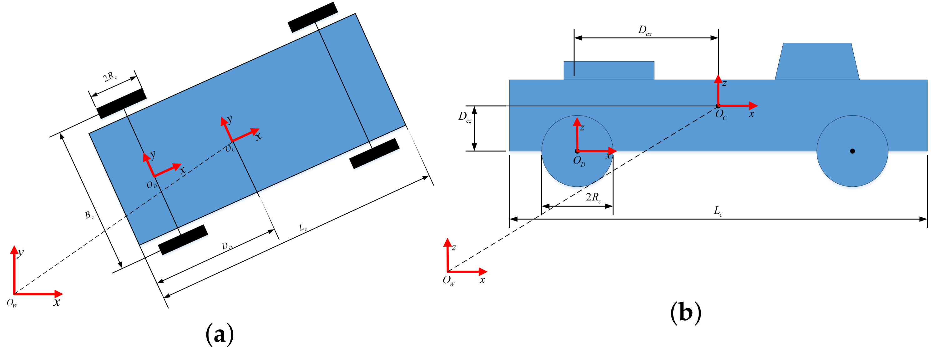
2.1. System Description

Currently, most mobile platforms use different wheels as driving and supporting mechanisms. However, mobile platforms with many driving wheels require more complicated synchronization control, are more expensive, and have fewer applications in daily life. Therefore, a typical mobile robot only uses the front wheels or the rear wheels as the driving wheels. The mobile robot is controlled by the rotation speed of the driving wheels. In general, the mobile platform’s rotational movement and forward movement can be precisely controlled by the driving wheels’ rotation speed. However, the basic movement of the mobile robot needs to avoid forward sliding and lateral slipping during movement.

Some coordinate frames need to be established in the working environment and on the mobile platform for positioning and trajectory tracking. These frames are as follows:

(1)

The world frame $O_W$: Establish the system’s global coordinate system at a fixed position in the inertial coordinate system; it is used to describe the position and posture of the mobile robot.

(2)

The driving-fixed frame $O_D$: Select the midpoint of the driving wheels as the origin of this local coordinate system, the x-axis direction is the same as the forward movement direction, the z-axis direction is the vertical direction of the movement plane, and the corresponding y-axis direction is established according to the right-hand rule direction.

(3)

The gravity-fixed frame $O_C$: The origin of the gravity-fixed frame is established at the gravity center of the mobile platform, the x-axis direction is the same as the forward direction, the z-axis direction is the vertical direction of the movement plane, and the corresponding y-axis direction is established according to the right-hand rule direction.

During movement, some structural parameters must be determined by measurement instead of using the values provided by the manufacturer to solve the positioning problem and achieve trajectory tracking with a mobile platform including the following:

(1)

Basic structure parameters: The length of the mobile platform is $L_c$, the width of the mobile platform is $B_c$, the radius of the wheels of the mobile platform is $R_c$, and the distance from the midpoint of the driving wheels to the gravity center of the mobile platform is $(D_{cx},D_{cy},D_{cz})$.

(2)

Vehicle positioning parameters: The initial position and initial posture of the midpoint of the driving wheels are $(P_{dx0},P_{dy0},Q_{dz0})$.

In the trajectory tracking task, the structural parameters are fixed values, and the position and posture of the mobile platform are constantly changing. However, the distance from the midpoint of the driving wheels to the gravity center of the mobile platform is also a fixed value. The specific description of the structural parameters is shown in Figure 1.

2.2. Kinematic Model

2.2.1. Discrete kinematics Model of Mobile Platform

(1)

Ideal kinematics discrete model

For an ideal mobile platform, the midpoint of the driving wheels coincides with the gravity center of the mobile platform on the $xy$ plane. Assuming the robot is moving on the $xy$ plane, the linear velocity and angular velocity can be expressed as follows:

$$\left\{\begin{array}{c}{\dot{P}}_{xc}\left(t\right)=V_c\left(t\right)cos\left(q_{zc}\left(t\right)\right)\\ {\dot{P}}_{yc}\left(t\right)=V_c\left(t\right)sin\left(q_{zc}\left(t\right)\right)\\ {\dot{\theta }}_{cz}\left(t\right)=W_c\left(t\right)\end{array}\right.\iff \left[\begin{array}{c}{\dot{P}}_{xc}\left(t\right)\\ {\dot{P}}_{yc}\left(t\right)\\ {\dot{\theta }}_{zc}\left(t\right)\end{array}\right]=\left[\begin{array}{cc}\begin{array}{c}cos\left({\theta }_{zc}\left(t\right)\right)\\ sin\left({\theta }_{zc}\left(t\right)\right)\\ 0\end{array}& \begin{array}{c}0\\ 0\\ 1\end{array}\end{array}\right]\left[\begin{array}{c}{V}_c\left(t\right)\\ W_c\left(t\right)\end{array}\right]$$

(1)

where ${\dot{P}}_{xc}$, ${\dot{P}}_{yc}$ is the linear velocity of the mobile platform along the x axis or the y axis of the world frame, ${\dot{\theta }}_{zc}$ is the angular velocity of rotation around the z axis of the world frame, $V_c$ is the linear velocity of the mobile platform, and $W_c$ is the rotation angle velocity of the mobile platform.

Considering control by two driving wheels, the linear velocity and angular velocity of the system can be directly described by the rotation speed of two driving wheels, which is explicitly expressed as follows:

$$\left\{\begin{array}{c}{V}_c\left(t\right)=\frac{R_c(W_L\left(t\right)+W_R\left(t\right))}{2}\\ W_c\left(t\right)=\frac{R_c(W_L\left(t\right)-W_R\left(t\right))}{2B_c}\end{array}\right.\iff \left[\begin{array}{c}{V}_c\left(t\right)\\ W_c\left(t\right)\end{array}\right]=\frac{R_c}{2}\left[\begin{array}{cc}1& 1\\ 1/B_c& -1/B_c\end{array}\right]\left[\begin{array}{c}{W}_L\left(t\right)\\ W_R\left(t\right)\end{array}\right]$$

(2)

where $W_L$ and $W_R$ are the actual rotational speed of the left and right driving wheels, respectively; $R_c$ is the radius of two driving wheels; and $B_c$ is the distance between two driving wheels of the mobile platform.

To control the mobile platform, we performed the kinematic modeling by combining Formulas (1) and (2) for directly driving the wheels, which can be expressed as follows:

$$\left[\begin{array}{c}{\dot{P}}_{xc}\left(t\right)\\ {\dot{P}}_{yc}\left(t\right)\\ {\dot{\theta }}_{zc}\left(t\right)\end{array}\right]=\frac{R_c}{2}\left[\begin{array}{cc}\begin{array}{c}cos\left({\theta }_{zc}\left(t\right)\right)\\ sin\left({\theta }_{zc}\left(t\right)\right)\\ 1/B_c\end{array}& \begin{array}{c}cos\left({\theta }_{zc}\left(t\right)\right)\\ sin\left({\theta }_{zc}\left(t\right)\right)\\ -1/B_c\end{array}\end{array}\right]\left[\begin{array}{c}{W}_L\left(t\right)\\ W_R\left(t\right)\end{array}\right]$$

(3)

In the actual movement, we need to convert continuous motion into discrete motion for controlling the mobile platform. In this case, the rotation speeds of the left wheel and the right wheel are regarded as the control variables; the linear velocity along the x axis and y axis of the world frame is denoted as ${\dot{p}}_{xc}\left(k\right)$ and ${\dot{p}}_{yc}\left(k\right)$, respectively; and the angular velocity around the z axis of the world frame is ${\dot{q}}_{zc}\left(k\right)$. Thus, the linear velocity and the angular velocity of the mobile platform can be expressed as follows:

$$\left[\begin{array}{c}{\dot{p}}_{xc}\left(k\right)\\ {\dot{p}}_{yc}\left(k\right)\\ {\dot{q}}_{zc}\left(k\right)\end{array}\right]=\frac{R_c}{2}\left[\begin{array}{cc}\begin{array}{c}cos\left(q_{zc}\left(k\right)\right)\\ sin\left(q_{zc}\left(k\right)\right)\\ 1/B_c\end{array}& \begin{array}{c}cos\left(q_{zc}\left(k\right)\right)\\ sin\left(q_{zc}\left(k\right)\right)\\ -1/B_c\end{array}\end{array}\right]\left[\begin{array}{c}{\dot{q}}_{cl}\left(k\right)\\ {\dot{q}}_{cr}\left(k\right)\end{array}\right]$$

(4)

where $q_{zc}$ is the rotation angle of the mobile platform at this time; ${\dot{q}}_{cl}$ and ${\dot{q}}_{cr}$ are the rotation velocity of the left and right wheel at this time, respectively.

When the rotation velocity of the driving wheels is regarded as the mobile platform’s control variable, $p_{xc}$ and $p_{yc}$ are the position of the mobile platform along the x axis and the y axis of the world frame, respectively; and $q_{zc}$ is the rotation angle of the z axis. Therefore, the discrete kinematics model of the mobile platform at $(k+1)$ time can be described as follows:

$$\left[\begin{array}{c}{p}_{xc}(k+1)\\ p_{yc}(k+1)\\ q_{zc}(k+1)\end{array}\right]=\left[\begin{array}{c}{p}_{xc}\left(k\right)\\ p_{yc}\left(k\right)\\ q_{zc}\left(k\right)\end{array}\right]+d_k·\frac{R_c}{2}\left[\begin{array}{cc}\begin{array}{c}cos\left(q_{zc}\left(k\right)\right)\\ sin\left(q_{zc}\left(k\right)\right)\\ 1/B_c\end{array}& \begin{array}{c}cos\left(q_{zc}\left(k\right)\right)\\ sin\left(q_{zc}\left(k\right)\right)\\ -1/B_c\end{array}\end{array}\right]\left[\begin{array}{c}{\dot{q}}_{cl}\left(k\right)\\ {\dot{q}}_{cr}\left(k\right)\end{array}\right]$$

(5)

where $d_k$ is the sampling time during the movement of the mobile platform.

(2)

Practical kinematics discrete model

For a practical mobile platform, the midpoint of the two driving wheels cannot wholly coincide with the actual gravity center of the mobile platform. As shown in Figure 1, an offset may be created between the midpoint of the driving axis and the gravity center of the mobile platform, $D_{cz}$ is the offset at the vertical height (the z axis of the driving-fixed frame), $D_{cx}$ is the offset at the horizontal direction (the x axis of the driving-fixed frame), and $D_{cy}$ is the offset at the y axis of the driving-fixed frame.

Assuming that the mobile platform is moving in the horizontal plane, the impact of $D_{cx}$ needs to be considered, but that of $D_{cz}$ should be ignored in the kinematic modeling of the mobile platform. Therefore, if the gravity center coincides with the midpoint of the driving wheels, Formula (6) can be used to describe the position and posture of the gravity center of the mobile platform at $(k+1)$ time, which is expressed as follows:

$$\left[\begin{array}{c}{p}_{xd}(k+1)\\ p_{yd}(k+1)\\ q_{zd}(k+1)\end{array}\right]=\left[\begin{array}{c}{p}_{xd}\left(k\right)\\ p_{yd}\left(k\right)\\ q_{zd}\left(k\right)\end{array}\right]+d_k\frac{R_c}{2}\left[\begin{array}{cc}\begin{array}{c}cos\left(q_{zd}\left(k\right)\right)\\ sin\left(q_{zd}\left(k\right)\right)\\ 1/B_c\end{array}& \begin{array}{c}cos\left(q_{zd}\left(k\right)\right)\\ sin\left(q_{zd}\left(k\right)\right)\\ -1/B_c\end{array}\end{array}\right]\left[\begin{array}{c}{\dot{q}}_{cl}\left(k\right)\\ {\dot{q}}_{cr}\left(k\right)\end{array}\right]$$

(6)

where $p_{xd}$ and $p_{yd}$ indicate the midpoint location of the driving wheel axis in the $xy$ plane, and $q_{zd}$ indicates the angle rotation around the z axis of the driving-fixed frame.

Suppose the gravity center does not coincide with the midpoint of the two driving wheels. In this case, to the actual position of the gravity center, the corresponding offset needs to be added to the kinematics model, which is expressed as follows:

$$\left[\begin{array}{c}{p}_{xc}\left(k\right)\\ p_{yc}\left(k\right)\\ q_{zc}\left(k\right)\end{array}\right]=\left[\begin{array}{c}{p}_{xd}\left(k\right)\\ p_{yd}\left(k\right)\\ q_{zd}\left(k\right)\end{array}\right]+\left[\begin{array}{ccc}cos\left(q_{zd}\left(k\right)\right)& -sin\left(q_{zd}\left(k\right)\right)& 0\\ sin\left(q_{zd}\left(k\right)\right)& cos\left(q_{zd}\left(k\right)\right)& 0\\ 0& 0& 1\end{array}\right]\left[\begin{array}{c}{D}_{cx}\\ D_{cy}\\ 0\end{array}\right]$$

(7)

where $p_{xc}$ and $p_{yc}$ are the position of the gravity center of the mobile robot in the $xy$ plane, and $q_{zc}$ is the rotation angle of the mobile robot.

Remark 1.

When selecting the position and posture of the gravity center as the output variable, the offset between the midpoint of driving wheels and the gravity center of the mobile platform needs to be considered. To reduce the complexity of the trajectory tracking problem, the position and posture of the midpoint of driving wheels in the world frame are regarded as the desired output variables.

2.2.2. State Equation of the Mobile Platform

(1)

Ideal state equation without disturbance

Converting the discrete kinematics model into the state equation, we redefine various variables of the mobile platform, where $u\left(k\right)={\left[{\dot{q}}_{cl}\left(k\right)),{\dot{q}}_{cr}\left(k\right)\right]}^T$ is the input control variable, $y\left(k\right)={\left[p_{xc}\left(k\right),p_{yc}\left(k\right),q_{zc}\left(k\right)\right]}^T$ is the output variable, and $q\left(k\right)$ is the state variable of the system. Therefore, the discrete state equation of the mobile platform can be expressed as follows:

$$\left\{\begin{array}{c}q(k+1)=q\left(k\right)+d_k·B\left(q_k\right)·u\left(k\right)\\ y\left(k\right)=q\left(k\right)\end{array}\right.$$

(8)

where $B\left(q_k\right)$ is the the control matrix of the mobile platform, which can be expressed as follows:

$$B\left(q_k\right)=\frac{R_c}{2}\left[\begin{array}{cc}\begin{array}{c}cos\left(q_{zc}\left(k\right)\right)\\ sin\left(q_{zc}\left(k\right)\right)\\ 1/B_c\end{array}& \begin{array}{c}cos\left(q_{zc}\left(k\right)\right)\\ sin\left(q_{zc}\left(k\right)\right)\\ -1/B_c\end{array}\end{array}\right]$$

(9)

(2)

Practical state equation with disturbance

The primary parameters of the state equation include the wheel radius and the width of the mobile platform. However, the above parameters can only be obtained through actual measurement, and the specific error between the measured parameters and the actual parameter cannot be ignored. Therefore, the exact state equation of the mobile platform can be expressed as follows:

$$\left\{\begin{array}{c}q(k+1)=q\left(k\right)+d_k·\tilde{B}\left(q_k\right)·u\left(k\right)\\ y\left(k\right)=q\left(k\right)\end{array}\right.$$

(10)

where $\tilde{B}\left(q_k\right)$ is the estimated parameter of the corresponding mobile platform.

The external disturbances of various signals need to be added to the actual state equation, where $\beta \left(k\right)$ is the random disturbance in the state parameters of the system, and $\alpha \left(k\right)$ is the random disturbances in the initial parameters of the system. Considering the above disturbance parameters in Formula (10), we can express the practical state equation with disturbance as follows:

$$\left\{\begin{array}{c}q(k+1)=q\left(k\right)+d_k·B\left(q_k\right)·u\left(k\right)+\tilde{\beta }\left(k\right)\\ y\left(k\right)=q\left(k\right)+\tilde{\alpha }\left(k\right)\end{array}\right.$$

(11)

where $\tilde{\beta }\left(k\right)=\beta \left(k\right)+d_k·(\tilde{B}\left(q_k\right)-B\left(q_k\right))·u\left(k\right)$ is the sum of the state disturbance and the system, and $\tilde{\alpha }\left(k\right)=\alpha \left(k\right)$ is the combination of the output disturbance and the measurement error of the system.

Remark 2.

The kinematics model is mainly used to construct the basic control model of the mobile platform. The control signal needs to be directly input to the actual mobile platform in trajectory tracking. Therefore, we did not need to perform high-precision tests on the above-mentioned physical structural parameters.

2.3. Actual Limitations

To obtain the actual physical limitations of the mobile platform, some constraints on the input variables and output variables must be described by formulas before performing the trajectory tracking task. Therefore, we specifically express various constraints as follows:

(1) Structure parameter limitations: The measurement error cannot be ignored when obtaining the radius of the driving wheels and the width of the mobile platform, which may be caused by the limitation of the measurement tool and the surveyor’s experience. Therefore, the measurement error must be in a particular range, which can be expressed as follows:

$$\left\{\begin{array}{c}max∥Bc-\tilde{B}c∥<b_{Bc}\\ max∥Rc-\tilde{R}c∥<b_{Rc}\end{array}\right.\Rightarrow max∥B\left(q_k\right)∥<b_B$$

(12)

where $b_{Bc},b_{Rc}$ is the maximum error of the actual estimated parameters, and $b_B$ is the maximum error of the control object.

(2) Signal disturbance limitations: The external environment is one of the key factors that cause other disturbances in the system. Therefore, the random disturbance of the state parameters and the output variable of the system are also within a specific constraint range, defined as follows:

$$\left\{\begin{array}{c}max∥\beta \left(k\right)∥<b_{\beta }\\ max∥\alpha \left(k\right)∥<b_{\alpha }\end{array}\right.\Rightarrow \left\{\begin{array}{c}max∥\beta \left(k\right)+d_k(\tilde{B}\left(q_k\right)-B\left(q_k\right))·u\left(k\right)∥<{\tilde{b}}_{\beta }\\ max∥{\tilde{\alpha }}_i\left(k\right)∥=max∥\alpha \left(k\right)∥<{\tilde{b}}_{\alpha }\end{array}\right.$$

(13)

where $b_{\beta }$ is the maximum disturbance of the system state variable, and $b_{\alpha }$ is the maximum disturbance of the output signal.

(3) Motor physical limitations: Due to the limitations of the motor and the voltage of the driving wheels, the rotation speed of the driving wheels must have a maximum speed limitation, expressed as follows:

$$\left\{\begin{array}{c}max∥{\dot{q}}_{cl}\left(k\right)∥\le b_w\\ max∥{\dot{q}}_{cr}\left(k\right)∥\le b_w\end{array}\right.\iff max∥u_i\left(k\right)∥\le b_{u_d}$$

(14)

where $b_w$ is the maximum speed of the two driving wheels, and $b_{u_d}$ is representing the maximum norm of the two-wheel drive speed matrix. The driving wheels were produced as one model to improve the control accuracy of the mobile platform.

(4) Initial error limitations: During the trajectory tracking task, the initial position of the robot and the starting position of the given trajectory are kept within a certain error range, which can be expressed as follows

$$∥q_d\left(0\right)-q_k\left(0\right)∥\le C_{q_0}$$

(15)

where, $q_k\left(0\right)$ represents the initial position and posture of the robot in each iteration learning, $q_d\left(0\right)$ represents the starting position and posture of a given trajectory, and $C_{q_0}$ is the maximum norm of the initial error matrix of the system.

(5) Kinematics limitations: In the robot state Equation (11), the B matrix needs to meet $max∥B\left(q_k\right)∥<b_B$. Meanwhile, the function needs to satisfy the global Lipschitz condition

$$∥d_k·B\left(q_{i+1}\left(k\right)\right)-d_k·B\left(q_i\left(k\right)\right)∥\le C_B∥q_{i+1}\left(k\right)-q_i\left(k\right)∥$$

(16)

where $d_k$ is a constant that represents the sampling time, and $C_B$ is the maximum value.

3. Design of the Controller

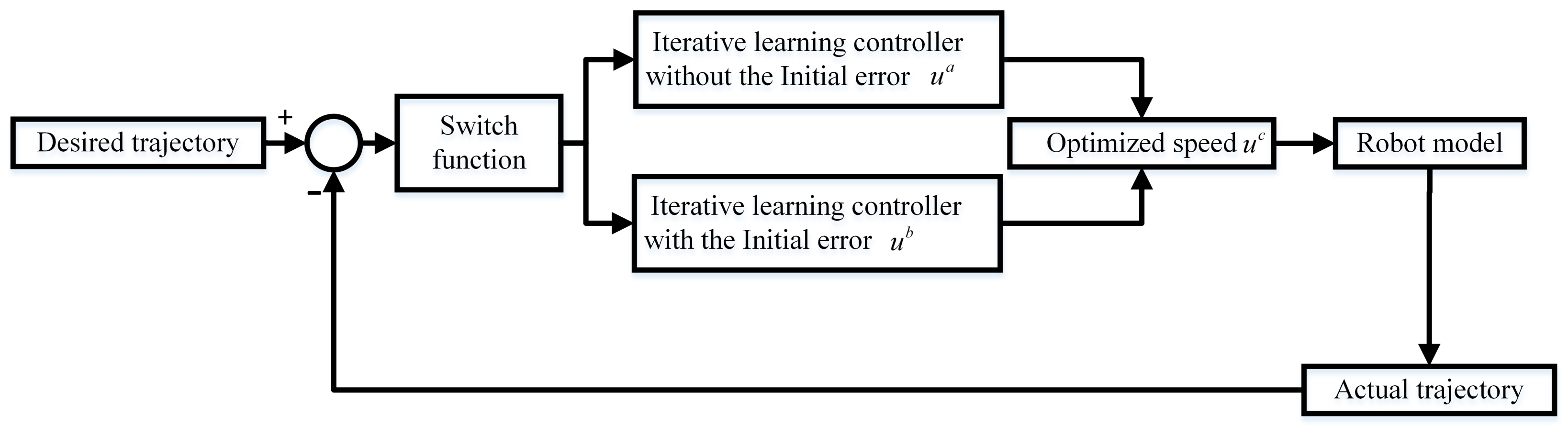
3.1. Design of the Hybrid Learning Iteration Controller for Mobile Platform

The hybrid controller has a two-layer hybrid structure that involves an iterative learning controller without initial error and an iterative learning controller with initial error; the basic structure of the hybrid controller is shown in Figure 2. To determine the choice of the corresponding controller, we designed the switch function based on the initial error of the mobile platform in different trajectory tracking tasks. When the initial error of the robot is equal to zero, the hybrid controller first uses the iterative controller without initial error to complete the assigned task. When the initial error exists in the system, it proceeds to the second type of iterative learning controller through the switching function. The specific design steps are as follows:

Step 1: Design the learning iteration controller without initial error. The basic aim of the iterative learning controller is to correct the actual input signal by iteratively learning the error between the ideal output signal and the actual input signal to perform the specified trajectory tracking task. Due to the different types of error parameters obtained, we can optimize the typical P-type learning control law by increasing different types of error signals. The optimized iterative learning controller can be expressed as follows:

$$u_{i+1}^a\left(k\right)=u_i^a\left(k\right)+L_1\left(k\right)e_i(k+1)+L_2\left(k\right)e_{i+1}\left(k\right)+L_3\left(k\right)e_{i+1}(k-1)$$

(17)

where $u_{i+1}^a\left(k\right)$ indicates the control speeds at k time in the next iteration, $e_i(k+1)$ indicates the error at $(k+1)$ time in the current iteration, $e_{i+1}\left(k\right)$ indicates the error at k time in the next iteration, $e_{i+1}(k-1)$ indicates the error at $(k-1)$ time in the next iteration, and $L_1\left(k\right),L_2\left(k\right),L_3\left(k\right)$ indicate the gain matrix of iterative learning in different error categories, and these gain matrices need to meet

$$∥L_1\left(k\right)∥\le b_{L_1},∥L_2\left(k\right)∥\le b_{L_2},∥L_3\left(k\right)∥\le b_{L_3}$$

(18)

where $b_{L_1}>0,b_{L_3}>0,b_{L_2}>0,k\in N$.

Theorem 1.

For the mobile robot described by Formula (11), in addition to satisfying the given kinematic characteristics and the specified constraint, the robot still satisfies the following conditions:

$$\left\{\begin{array}{c}∥I-[L_1\left(k\right)+L_2\left(k\right)+L_3\left(k\right)]B(q_i,k)∥\le \rho <1\\ y_i\left(0\right)=y_d\left(0\right),(i=0,1,2,\dots )\end{array}\right.$$

(19)

By using the iterations learning law (17), the output signal of the mobile system can be converted to the desired trajectory $y_d\left(k\right)(0\le k\le n)$, namely

$$\underset{k\to \infty }{lim}{y}_s\left(k\right)\to y_d\left(k\right)(0\le k\le n)$$

(20)

Proof. 

The proof of Theorem 1 is shown in Section 3.2 of the article. □

Step 2: Design the learning iteration controller with initial error. To achieve trajectory tracking, the initial error of the typical iterative control law (17) needs to be equal to zero. In the actual movement of the mobile platform, error may exist between the initial position of the mobile platform and the given trajectory. In this case, the iterative learning controller needs to compensate for the corresponding error in the initial moment to achieve trajectory tracking. Therefore, the iterative learning controller can be expressed as follows:

$$u_{i+1}^b\left(k\right)=u_i^b\left(k\right)+L_1\left(k\right)e_i(k+1)+e^{-kdt}\theta \left(k\right)L_1\left(k\right)e_i\left(0\right)$$

(21)

where $e_i\left(0\right)$ represents the initial error of each iteration learning process, and $\theta \left(k\right)$ represents the corresponding compensation function, which can be expressed as follows:

$$\theta \left(k\right)=\left\{\begin{array}{cc}\frac{2}{d_k\ast h}(1-\frac{k}{h}),& \left(0\le k\le h\right)\\ 0,& \left(h<k\le n\right)\end{array}\right.$$

(22)

Theorem 2.

For the mobile robot described by Formula (11), in addition to satisfying the given kinematic characteristics and the specified constraint, the robot still satisfies the following conditions:

$$\left\{\begin{array}{c}{y}_i\left(0\right)=y_d\left(0\right)\\ ∥I-L_1\left(k\right)B(q_i,k)∥\le \rho <1\end{array}\right.$$

(23)

By using the iterations learning law (21), the output signal of the mobile system can be converted to the desired trajectory $y_d\left(k\right)(0\le k\le n)$, namely

$$y_s\left(k\right)=\left\{\begin{array}{cc}{y}_d\left(k\right)+e^{-kdt}{L}_1\left(k\right)\sum _{j=h}^k\theta \left(k\right)(y_d\left(0\right)-y_i\left(0\right))& (0\le k\le h)\\ y_d\left(k\right)& (h<k\le n)\end{array}\right.$$

(24)

Proof. 

The proof of Theorem 2 is very similar as the proof of Theorem 1, but it is simpler than Section 3.2. The proof process can refer to the literature [38]. □

Step 3: Optimize the control speeds. The input control signals of the driving wheels can be obtained through the above two types of iterative controllers. Due to the limitation on the voltage and structural design of the drive motor in the actual robot system, the maximum speed of the motor movement is a given value, which can be expressed as $b_w$. Then, we need to optimize the control speeds solved by the iterative controller. To ensure the rotation movement of the mobile platform, the optimization signal needs to ensure the rotation speed ratio of the two driving wheels is the same as the solution result. Therefore, the optimized control speeds can be expressed as follows:

$$u^c\left(k\right)=\left\{\begin{array}{c}{\left[\begin{array}{cc}\frac{{\dot{q}}_{cl}\left(k\right)}{max({\dot{q}}_{cl}\left(k\right),{\dot{q}}_{cr}\left(k\right))}{b}_w,& \frac{{\dot{q}}_{cr}\left(k\right)}{max({\dot{q}}_{cl}\left(k\right),{\dot{q}}_{cr}\left(k\right))}{b}_w\end{array}\right]}^T,if(max({\dot{q}}_{cl}\left(k\right),{\dot{q}}_{cr}\left(k\right))\ge b_w);\\ {\left[\begin{array}{cc}{\dot{q}}_{cl}\left(k\right),& {\dot{q}}_{cr}\left(k\right)\end{array}\right]}^T,others;\end{array}\right.$$

(25)

where $u^c\left(k\right)$ represents the optimized system control signal, $b_w$ represents the maximum speed of the two driving wheels, ${\dot{q}}_{cl}\left(k\right)$ represents the speed of the left drive wheel, and ${\dot{q}}_{cr}\left(k\right)$ represents the speed of the right drive wheel of the system.

3.2. Theoretical Proof

To prove Theorem 1, we need to solve the error between the desired control signal and the actual control signal and analyze the error between the expected trajectory and the actual trajectory. The convergence of the controller is proved as follows:

Step 1: In solving the error between the desired control signal and the actual control signal, we need to use the state error of the system. Assuming $q_d$ represents the expected motion state of the system, the state error can be expressed as follows:

$$\begin{array}{c}\Delta q_i(k+1)=q_d(k+1)-q_i(k+1)\hfill \\ =[q_d\left(k\right)+d_k{B}_d{u}_d\left(k\right)]-(q_i\left(k\right)+d_k{B}_i{u}_i\left(k\right)+{\tilde{\beta }}_i\left(k\right))\hfill \\ =\Delta q_i\left(k\right)+(B_d-B_i)u_d\left(k\right)-B_i(u_d\left(k\right)-u_i\left(k\right))-{\tilde{\beta }}_i\left(k\right)\hfill \end{array}$$

(26)

According to the formula constraint expression, the state error of the system can be effectively scaled, which can be expressed as follows:

$$∥\Delta q_i(k+1)∥\le ∥\Delta q_i∥+C_B{b}_{u_d}∥\Delta q_i∥+b_B∥\Delta u_i∥+{\tilde{b}}_{\beta }$$

(27)

If we set $h_2=(1+C_B{b}_{u_d})$, the state error (27) can be simplified again, which can be expressed as follows:

$$∥\Delta q_i(k+1)∥\le h_2∥\Delta q_i∥+b_B∥\Delta u_i∥+{\tilde{b}}_{\beta }$$

(28)

Solving the state error by iteration method from the state error at the initial moment to the current moment, we obtain the state error expression:

$$\begin{array}{c}∥\Delta q_i∥\le (∥h_2{b}_B\Delta u_1∥+∥h_2^2{b}_B\Delta u_2∥+\dots \dots +∥h_2^{i-1}{b}_B\Delta u_{i-1}∥)\hfill \\ +h_2({\tilde{b}}_{\beta }+{\tilde{b}}_{\beta }+\dots \dots +{\tilde{b}}_{\beta })+h_2^k{b}_{q_0}\hfill \\ \le {\displaystyle \sum _{j=0}^{k-1}}(h_2^{k-1-j}[b_B∥\Delta u_i∥+{\tilde{b}}_{\beta }]+h_2^k{b}_{q_0}\hfill \end{array}$$

(29)

where $b_B$ represents the maximum error of the control object, ${\tilde{b}}_{\beta }$ is the maximum disturbance of the state variable, and $b_{q_0}$ indicates the error of the system at the initial time.

Step 2: Assuming that $u_d$ as the desired control signal can control the mobile platform to track the desired trajectory. The error between the actual control signal and the desired control signal can be expressed as follows:

$$\begin{array}{c}\Delta u_{i+1}\left(k\right)=u_d\left(k\right)-u_{i+1}\left(k\right)\hfill \\ =u_d\left(k\right)-u_i\left(k\right)-L_1{e}_i(k+1)-L_2{e}_{i+1}\left(k\right)-L_3{e}_{i+1}(k-1)\hfill \\ =u_d\left(k\right)-u_i\left(k\right)-L_1[y_d(k+1)-y_i(k+1)]\hfill \\ -L_2[y_d\left(k\right)-y_{i+1}\left(k\right)]-L_3[y_d(k-1)-y_{i+1}(k-1)]\hfill \\ =∥\Delta u_i∥-L_1(q_d(k+1)-q_i(k+1)-{\alpha }_i(k+1))\hfill \\ -L_2(q_d\left(k\right)-q_{i+1}\left(k\right)-{\alpha }_{i+1}(k+1))\hfill \\ -L_3(q_d(k-1)-q_{i+1}(k-1)-{\alpha }_{i+1}(k-1))\hfill \\ =∥\Delta u_i∥-L_1[∥\Delta q_i∥+(B_d-B_i)u_d+B_i∥\Delta u_i∥-{\alpha }_i\left(k\right)]\hfill \\ -L_2(∥\Delta q_{i+1}∥-{\alpha }_{i+1}(k+1))-L_3(∥\Delta q_{i-1}∥-{\alpha }_{i-1}(k-1))\hfill \\ =∥\Delta u_i∥-L_1∥\Delta q_i∥-L_1(B_d-B_i)u_d-L_1{B}_i∥\Delta u_i∥+L_1{\alpha }_i\left(k\right)\hfill \\ -L_2∥\Delta q_{i+1}∥+L_2{\alpha }_{i+1}(k+1)-L_3∥\Delta q_{i-1}∥+L_3{\alpha }_{i-1}(k-1)\hfill \\ =(1-L_1{B}_i)∥\Delta u_i∥-L_1∥\Delta q_i∥-L_1(B_d-B_i)u_d+L_1{\alpha }_i\left(k\right)\hfill \\ -L_2∥\Delta q_{i+1}∥+L_2{\alpha }_{i+1}(k+1)-L_3∥\Delta q_{i-1}∥+L_3{\alpha }_{i-1}(k-1)\hfill \end{array}$$

(30)

Considering physical constraints, Formula (30) can be simplified to the following:

$$\begin{array}{c}∥\Delta u_{i+1}\left(k\right)∥\le ∥I-L_1{B}_i∥∥\Delta u_i∥+b_{L1}∥\Delta q_i∥+b_{L1}{c}_B{b}_u∥\Delta q_i∥+b_{L1}{b}_{\alpha }\hfill \\ +b_{L2}∥\Delta q_{i+1}∥+b_{L2}{b}_{\alpha }+b_{L3}∥\Delta q_{i-1}∥+b_{L3}{b}_{\alpha }\hfill \\ =∥I-L_1{B}_i∥∥\Delta u_i∥+(b_{L1}+b_{L1}{c}_B{b}_u)∥\Delta q_i∥+b_{L2}∥\Delta q_{i+1}∥\hfill \\ +b_{L3}∥\Delta q_{i-1}∥+(b_{L1}{b}_{\alpha }+b_{L2}{b}_{\gamma }+b_{L3}{b}_{\alpha })\hfill \end{array}$$

(31)

If we set $h_1=b_{L1}+b_{L1}{c}_B{b}_u=b_{L1}(1+c_B{b}_u)$, $b_1=(b_{L1}{b}_{\alpha }+b_{L2}{b}_{\alpha }+b_{L3}{b}_{\alpha })$, Formula (31) can be simplified again as follows:

$$∥\Delta u_{i+1}\left(k\right)∥\le ∥I-L_1{B}_i∥∥\Delta u_i∥+h_1∥\Delta q_i∥+b_{L2}∥\Delta q_{i+1}∥+b_{L3}∥\Delta q_{i-1}∥+b_1$$

(32)

The Formula (32) contains the system output error function and the system state error function; however, we need to eliminate the system state error to obtain the output error function. Substitute the status error (29) into the above system Formula (32) to obtain the following:

$$\begin{array}{c}∥\Delta u_{i+1}\left(k\right)∥\le ∥I-L_1{B}_i∥∥\Delta u_i∥+h_1\left[{\displaystyle \sum _{j=0}^{k-1}}[h_2^{k-1-j}(b_B∥\Delta u_i∥+b_{\beta })+h_2^k{b}_{q_0}]\right]\hfill \\ +b_{L2}\left[{\displaystyle \sum _{j=0}^{k-1}}[h_2^{k-1-j}(b_B∥\Delta u_{i+1}∥+b_{\beta })+h_2^k{b}_{q_0}]\right]\hfill \\ +b_{L3}\left[{\displaystyle \sum _{j=0}^{k-2}}[h_2^{k-2-j}(b_B∥\Delta u_{i-1}∥+b_{\beta })+h_2^{k-1}{b}_{q_0}]+b_1\right]\hfill \\ =∥I-L_1{B}_i∥∥\Delta u_i∥+h1h_2^k{b}_{q_0}+B_{L2}{h}_2^k{b}_{q_0}{B}_{L3}{h}_2^{k-1}{b}_{q_0}{b}_1\hfill \\ +h_1{\displaystyle \sum _{j=0}^{k-1}}{h}_2^{k-1-j}(b_B∥\Delta u_i∥+b_{\beta })+b_{L2}{\displaystyle \sum _{j=0}^{k-1}}[h_2^{k-1-j}(b_B∥\Delta u_{i+1}∥+b_{\beta })\hfill \\ +b_{L3}{\displaystyle \sum _{j=0}^{k-2}}[h_2^{k-2-j}(b_B∥\Delta u_{i+1}∥+b_{\beta })\hfill \end{array}$$

(33)

Multiply the left and right sides of the above Formula (33) by $\frac{1}{{\lambda }^k}$, which can, thus, be solved to obtain the following:

$$\begin{array}{c}∥\Delta u_{i+1}\left(k\right)∥\left(\frac{1}{{\lambda }^k}\right)\le ∥I-L_1{B}_i∥∥\Delta u_i∥\left(\frac{1}{{\lambda }^k}\right)+h_1\frac{h_2^k}{{\lambda }^k}{b}_{q_0}+b_{L2}\frac{h_2^k}{{\lambda }^k}{b}_{q_0}+b_{L3}\frac{h_2^{k-1}}{{\lambda }^k}{b}_{q_0}\hfill \\ +b_1\left(\frac{1}{{\lambda }^k}\right)+h_1{\displaystyle \sum _{j=0}^{k-1}}\frac{h_2^{k-1-j}}{{\lambda }^k}(b_B∥\Delta u_i∥+b_{\beta })+b_{L2}{\displaystyle \sum _{j=0}^{k-1}}\frac{h_2^{k-1-j}}{{\lambda }^k}(b_B∥\Delta u_{i+1}∥+b_{\beta })\hfill \\ +b_{L3}{\displaystyle \sum _{j=0}^{k-2}}\frac{h_2^{k-2-j}}{{\lambda }^k}(b_B∥\Delta u_{i+1}∥+b_{\beta })\hfill \\ =∥I-L_1{B}_i∥∥\Delta u_i∥\left(\frac{1}{{\lambda }^k}\right)+h_1\frac{h_2^k}{{\lambda }^k}{b}_{q_0}+b_{L2}\frac{h_2^k}{{\lambda }^k}{b}_{q_0}+b_{L3}\frac{h_2^{k-1}}{{\lambda }^{k-1}}{b}_{q_0}\left(\frac{1}{{\lambda }^k}\right)\hfill \\ +b_1\left(\frac{1}{{\lambda }^k}\right)+\frac{h_1}{\lambda }{\displaystyle \sum _{j=0}^{k-1}}\frac{h_2^{k-1-j}}{{\lambda }^{k-1-j}}(b_B\frac{∥\Delta u_i∥}{{\lambda }^j}+\frac{b_{\beta }}{{\lambda }^j})+\frac{b_{L2}}{\lambda }{\displaystyle \sum _{j=0}^{k-1}}\frac{h_2^{k-1-j}}{{\lambda }^{k-1-j}}(b_B\frac{∥\Delta u_{i+1}∥}{{\lambda }^j}+\frac{b_{\beta }}{{\lambda }^j})\hfill \\ +\frac{b_{L3}}{{\lambda }^2}{\displaystyle \sum _{j=0}^{k-2}}\frac{h_2^{k-2-j}}{{\lambda }^{k-2-j}}(b_B\frac{∥\Delta u_{i+1}∥}{{\lambda }^j}+\frac{b_{\beta }}{{\lambda }^j})\hfill \\ =\rho {∥\Delta u_i∥}_{\lambda }+h_1{b}_{q_0}+b_{L2}{b}_{q_0}+b_{L3}{b}_{q_0}\left(\frac{1}{{\lambda }^k}\right)+b_1\left(\frac{1}{{\lambda }^k}\right)\hfill \\ +\frac{h_1}{\lambda }(b_B{∥\Delta u_i∥}_{\lambda }+b_{\beta }){\displaystyle \sum _{j=0}^{k-1}}\frac{h_2^{k-1-j}}{{\lambda }^{k-1-j}}+\frac{b_{L2}}{\lambda }(b_B{∥\Delta u_{i+1}∥}_{\lambda }+b_{\beta }){\displaystyle \sum _{j=0}^{k-1}}\frac{h_2^{k-1-j}}{{\lambda }^{k-1-j}}\hfill \\ +\frac{b_{L3}}{{\lambda }^2}(b_B{∥\Delta u_{i-1}∥}_{\lambda }+b_{\beta }){\displaystyle \sum _{j=0}^{k-2}}\frac{h_2^{k-2-j}}{{\lambda }^{k-2-j}}\hfill \\ \le \rho {∥\Delta u_i∥}_{\lambda }+h_1{b}_{q_0}+b_{L2}{b}_{q_0}+b_{L3}{b}_{q_0}+b_1\hfill \\ +(b_B{∥\Delta u_i∥}_{\lambda }+b_{\beta })\left(\frac{h_1[1-{(h_2/\lambda )}^n]}{\lambda -h_2}\right)+(b_B{∥\Delta u_{i+1}∥}_{\lambda }+b_{\beta })\left(\frac{b_{L2}[1-{(h_2/\lambda )}^n]}{\lambda -h_2}\right)\hfill \\ +(b_B{∥\Delta u_{i+1}∥}_{\lambda }+b_{\beta })\left(\frac{b_{L3}[1-{(h_2/\lambda )}^n]}{\lambda -h_2}\right)\hfill \\ =(\rho +\frac{b_B{h}_1}{\lambda -h_2})∥\Delta u_i∥+\frac{(b_B{b}_{L2}+b_B{b}_{L3})[1-{(h_2/\lambda )}^n]}{\lambda -h_2}{∥\Delta u_{i+1}∥}_{\lambda }\hfill \\ +h_1{b}_{q_0}+b_{L2}{b}_{q_0}+b_{L3}{b}_{q_0}+b_1+\frac{b_{\beta }(h_1+b_{L2}+b_{L3})[1-{(h_2/\lambda )}^n]}{\lambda -h_2}\hfill \end{array}$$

(34)

If we set $\lambda >max\{1,h_2,b_B(b_{L2}+b_{L3})\}$, we can obtain the following:

$$\left[1-\frac{b_B(b_{L2}+b_{L3})[1-{(h_2/\lambda )}^n]}{\lambda -h_2}\right]>0\Rightarrow \left\{\begin{array}{c}\alpha -h_2\ne 0\\ \alpha >h_2+b_B(b_{L2}+b_{L3})\\ \alpha -h_2>b_B(b_{L2}+b_{L3})[1-{(h_2/\lambda )}^n]\end{array}\right.$$

(35)

Then, the above inequality (35) can be simplified as follows:

$${∥\Delta u_{i+1}\left(k\right)∥}_{\lambda }\le A{∥\Delta u_i\left(k\right)∥}_{\lambda }+B$$

(36)

where

$$A=\frac{\left[\rho +\frac{b_B{h}_1}{\lambda -h_2}\right]}{\left[1-\frac{b_B(b_{L2}+b_{L3})[1-{(h_2/\lambda )}^n]}{\lambda -h_2}\right]},B=\frac{\left[h_1{b}_{q_0}+b_{L2}{b}_{q_0}+b_{L3}{b}_{q_0}+b_1+\frac{b_{\beta }(h_1+b_{L2}+b_{L3})[1-{(h_2/\lambda )}^n]}{\lambda -h_2}\right]}{\left[1-\frac{b_B(b_{L2}+b_{L3})[1-{(h_2/\lambda )}^n]}{\lambda -h_2}\right]}$$

(37)

Iterating the output error from the initial moment to the current moment, the output error at any moment can be obtained:

$${∥\Delta u_{i+1}\left(k\right)∥}_{\lambda }\le A{∥\Delta u_i\left(k\right)∥}_{\lambda }+B=A^i{∥\Delta u_1\left(k\right)∥}_{\lambda }+\frac{B(1-A^i)}{1-A}$$

(38)

If we set $\lambda$ to be very large and the system parameter $A\approx \rho <1$, Formula (38) can be simplified as follows:

$$\underset{i\to \infty }{lim}{∥\Delta u_i\left(k\right)∥}_{\lambda }\le \frac{B}{1-A}$$

(39)

When the output disturbance $b_{\alpha }=0$, the initial error $b_{q_0}=0$ and the state disturbance signal $b_{\beta }=0$ are brought into Formulas (37) and (39), the output error of the controller is proved to approach zero asymptotically. Namely, the actual output of the controller is infinitely close to the desired control signal.

Step 3: In analyzing the error between the actual trajectory and the expected trajectory, we need to use the state error of the system. According to Formulas (29) and (39), we can find the expression of the state error. To analyze the output error of the system, we also need to multiply the state error by ${\left(\lambda \right)}^{-k}$. Then, the expression can be simplified as follows:

$$\begin{array}{c}∥\Delta q_i∥\left(\frac{1}{{\lambda }^k}\right)\le {\displaystyle \sum _{j=0}^{k-1}}\frac{h_2^{k-1-j}}{{\lambda }^{k-1-j}}(b_B\frac{∥\Delta u_i∥}{{\lambda }^j}+b_{\beta }\frac{1}{{\lambda }^j})+\frac{h_2^k}{{\lambda }^k}{b}_{q_0}\hfill \\ \le (b_B{∥\Delta u_i∥}_{\lambda }+b_{\beta }){\displaystyle \sum _{j=0}^{k-1}}\frac{h_2^{k-1-j}}{{\lambda }^{k-1-j}}+b_{q_0}\hfill \\ =b_B\frac{[1-{(h_2/\lambda )}^n]}{\lambda -h_2}{∥\Delta u_i∥}_{\lambda }+b_{\beta }\frac{[1-{(h_2/\lambda )}^n]}{\lambda -h_2}+b_{q_0}\hfill \end{array}$$

(40)

After infinite iterations, the state error of system can be simplified to the following:

$$\underset{i\to \infty }{lim}{∥\Delta q_i∥}_{\lambda }\le b_B\frac{[1-{(h_2/\lambda )}^n]}{\lambda -h_2}\frac{B}{1-A}+b_{\beta }\frac{[1-{(h_2/\lambda )}^n]}{\lambda -h_2}+b_{q_0}$$

(41)

where $b_B$ represents the maximum norm of the control matrix, $b_{\beta }$ represents the maximum norm of the state disturbance, and $b_{q_0}$ represents the initial error of the system. Assuming the initial error in the Formula (41) is $b_{\alpha }=0,b_{\beta }=0,b_{q_0}=0$, the actual state output of the system is consistent with the expected state output.

Step 4: To prove that the controller can track the desired trajectory, we need to analyze the output error of the system, which can be expressed as follows:

$$\begin{array}{c}∥\Delta y_i\left(k\right)∥=y_d\left(k\right)-y_i\left(k\right)=q_d\left(k\right)-(q_i\left(k\right)+{\alpha }_i\left(k\right))\hfill \\ =∥\Delta q_i\left(k\right)∥-b_{\alpha }\hfill \end{array}$$

(42)

After infinite iterations, the output error can be simplified to the following:

$$\underset{i\to \infty }{lim}{∥\Delta y_i∥}_{\lambda }\le \underset{i\to \infty }{lim}{∥\Delta q_i∥}_{\lambda }-b_{\alpha }$$

(43)

where $b_{\alpha }$ represents the maximum norm of the output disturbance signal of the system. If the maximum norm of output disturbance signal is $b_{\alpha }=0$, the output error of the system is close to the state error. When the state error of the third step is $\underset{i\to \infty }{lim}{∥\Delta q_i∥}_{\lambda }=0$, the actual trajectory of the robot can follow the expected trajectory.

Comparing the output error signal of the controller (39), the state error (41), and the output error (43) of the system, we can find that: (1) When the output disturbance $b_{\alpha }=0$, the initial error $b_{q_0}=0$ and the state disturbance signal $b_{\beta }=0$, the actual control signal will converge to the desired control signal. (2) When the output disturbance $b_{\alpha }=0$, the initial error $b_{q_0}=0$ and the state disturbance signal $b_{\beta }=0$, the output signal of the system will converge to the expected trajectory.

4. Experimental Results

To validate the performance of the hybrid controller, we designed some experiments with various tracking trajectories by directly control the driving wheels. To enable the general use of the controller, we selected a personal computer to simulate the performance. The computer was equipped with an Intel(R) Core(TM) i5-7500, CPU @3.4HZ, RAM @8G, and the basic configuration was the a medium type in terms of computing performance. The basic parameters of the mobile platform are specifically expressed as follows:

$$\begin{array}{c}{L}_c=1.104\mathrm{m};\hspace{1em}{B}_c=0.518\mathrm{m};\hspace{1em}{R}_c=0.200\mathrm{m};\\ D_{cx}=0.340\mathrm{m};\hspace{1em}{D}_{cy}=0.00\mathrm{m};\hspace{1em}{D}_{cz}=0.119\mathrm{m};\hspace{1em}{u}_{max}=180\mathrm{rad}/\mathrm{s};\end{array}$$

(44)

The flowing subsection summarizes the processes and the results of these typical simulations.

4.1. Basic Performance Test

To test the basic performance of the iterative controller proposed in this paper, we conducted the first simulation experiment for various trajectory tracking tasks by directly driving the two wheels of the mobile robot shown in Figure 3. Four typical trajectory tracking tasks were used in the first simulation: circular trajectory, combination trajectory of arc and straight, cardioid-like trajectory, and spiral-like trajectory.

Trajectory 1: The circular trajectory is a closed path composed of a single arc. The circle’s center is $P_{C1}(0,0)$, the radius length is $R_1=10$ m, and the initial point is $P_0(0,10)$. The mobile platform needs to return to the initial position by rotating ${360}^{\circ }$ in the counterclockwise direction of the circular trajectory, the total time of the trajectory is $t_s=2$ s, the sampling time is $d_t=0.001$ s, and the initial position and posture of the mobile platform is $(0,10,\pi /2)$.

Trajectory 2: The combination trajectory of arc and straight is also a closed path composed of two arcs and two straight lines. In this path, the center of first arc is $P_{C1}(0,0)$, and the radius is $R_1=5$ m; the center of second arc is $P_{C2}(0,-10)$, the radius is $R2=5$ m; the two straight lines connect the upper points and the lower points of the two arcs. The mobile platform needs to rotate ${360}^{\circ }$ in the counterclockwise direction along the combination trajectory and return to the initial position. The time of each arc is $t_{C1}=t_{C2}=0.5$ s, the time of each straight line is $t_{L1}=t_{L2}=1$ s, the total time of the combination trajectory is $t_s=3$ s, the sampling time is $d_t=0.001$ s, and the initial position and posture of the mobile platform are $(0,5,\pi /2)$.

Trajectory 3: The cardioid-like trajectory is a closed path composed of multiple semicircles. In this path, the center of the first semicircle is $P_{C1}(0,0)$, the radius is $R_1=2.5$ m, and the starting point of the first semicircle is (2.5,0). The mobile platform arrives at the endpoint of the first semicircle trajectory by rotating ${180}^{\circ }$ in the counterclockwise direction. The starting point of the second semicircle is set as the first endpoint, the center of the second semicircle is $P_{C2}(2.5,0)$, and the radius is $R_2=5$ m. The mobile robot rotates ${180}^{\circ }$ in the counterclockwise direction to the endpoint of the second semicircle trajectory. The starting point of the third semicircle is set as the second endpoint, the center of the third semicircle is $P_{C3}(5,0)$, and the radius is $R_3=2.5$ m. The mobile robot returns to the initial position of the cardioid-like trajectory by rotating ${180}^{\circ }$ in the counterclockwise direction. The duration for first and third semicircle is $t_{C1}=t_{C3}=0.5$ s, the time of the second semicircle is $t_{C2}=1$ s, the total time is $t_s=2$ s, the sampling time is $d_t=0.001$ s, and the initial position and posture of the mobile platform are $(2.5,0,\pi /2)$.

Trajectory 4: The spiral-like trajectory is an open path composed of multiple semicircles. In this path, the center of the first semicircle is $P_{C1}(0,0)$, the radius is $R_1=3$ m, and the starting point of first semicircle is $(2.5,0)$. The mobile platform arrives at the endpoint of the first semicircle trajectory by rotating ${180}^{\circ }$ in the counterclockwise direction. The starting point of the second semicircle is set as the first endpoint, the center of the second semicircle is $P_{C2}(0.5,0)$, and the radius is $R_2=3.5$ m. The mobile platform rotates ${180}^{\circ }$ in the counterclockwise direction to the endpoint of the second semicircle trajectory. The starting point of the third semicircle is set as the second endpoint, the center position of the third semicircle is $P_{C3}(0,0)$, and the radius is $R_3=4$. Then, the mobile platform needs to rotate ${180}^{\circ }$ in the counterclockwise direction to the endpoint of the third semicircle trajectory. The starting point of the fourth semicircle is set as the third endpoint, the center position of the forth semicircle is $P_{C4}(0,0)$, and the radius is $R_4=4$ m.

Then, the mobile robot reaches the endpoint of the spiral trajectory by rotating ${180}^{\circ }$ in the counterclockwise direction. The time of each semicircle is $t_{C1}=t_{C2}=t_{C3}=t_{C4}=0.5$ s, the total time of the spiral trajectory is $t_s=2$ s, the sampling time is $d_t=0.001$ s, and the initial position and posture of the mobile platform is $(3,0,\pi /2)$.

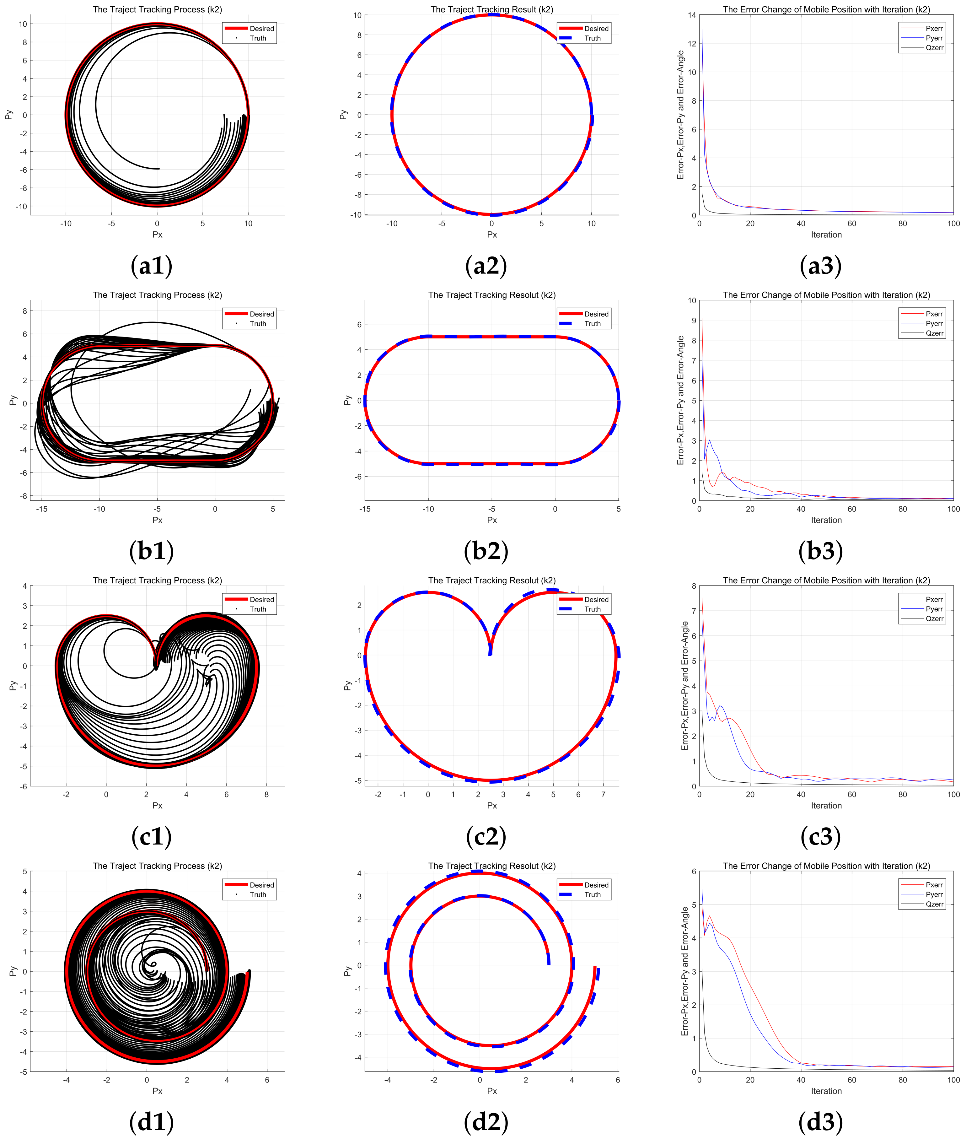
4.1.1. Performance Test of the Hybrid Controller without Initial Error

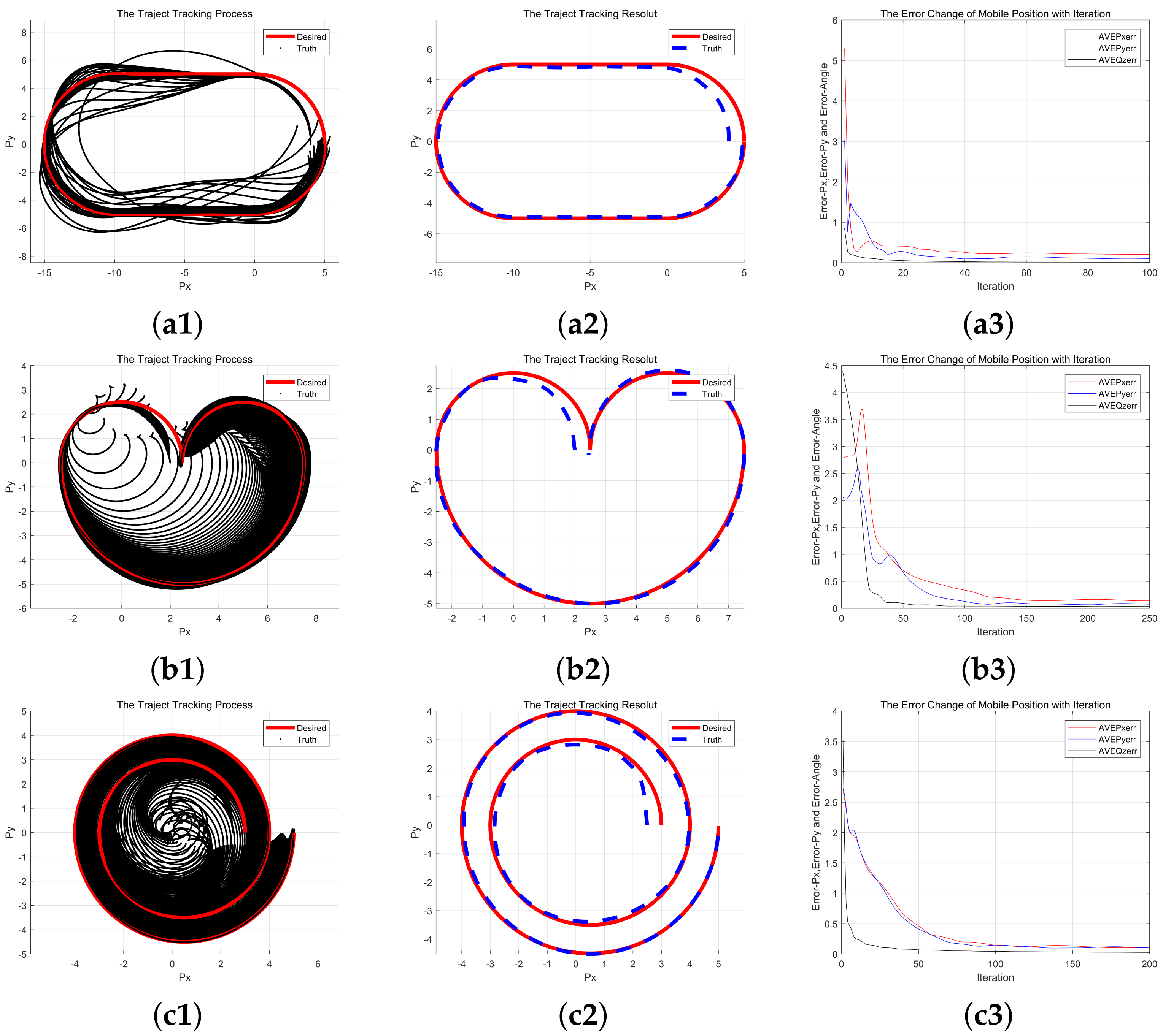
Assuming there is no initial error in the various trajectories, the typical iterative learning controller (17) directly controls the rotation speed of the two wheels to solve the trajectory tracking problem.

Situation 1: The control law of the corresponding gain matrix is described as follows:

$$L_1\left(k\right)=\frac{1}{R_{rs}}\left[\begin{array}{c}\begin{array}{ccc}cos\left(q\right)& sin\left(q\right)& B_{rs}\end{array}\\ \begin{array}{ccc}cos\left(q\right)& sin\left(q\right)& -B_{rs}\end{array}\end{array}\right];L_2\left(k\right)=0;L_3\left(k\right)=0;$$

(45)

where $R_{rs}=R_c$ represents the actual radius of the wheels, and $B_{rs}=B_c$ represents the actual distance between the driving wheels.

The trajectory tracking process and the final result of the mobile platform after 100 iteration process are shown in Figure 3. By comparing the tracking results, we found the following:

(1)

The system can directly control two driving wheels to track the specified trajectories without initial error using the iterative learning controller.

(2)

Selecting the midpoint of the two driving wheels as the control variable can effectively achieve different trajectory tracking tasks.

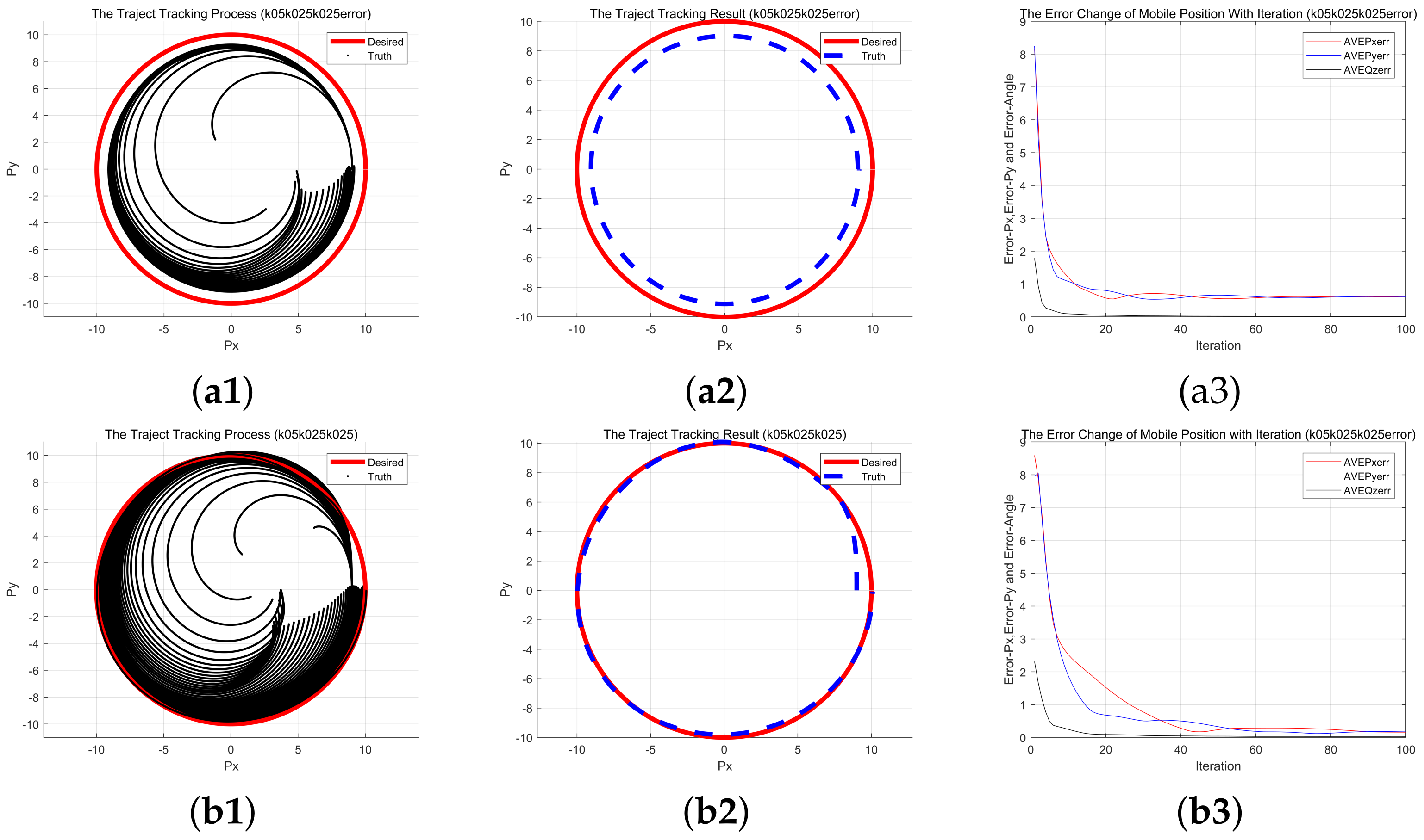
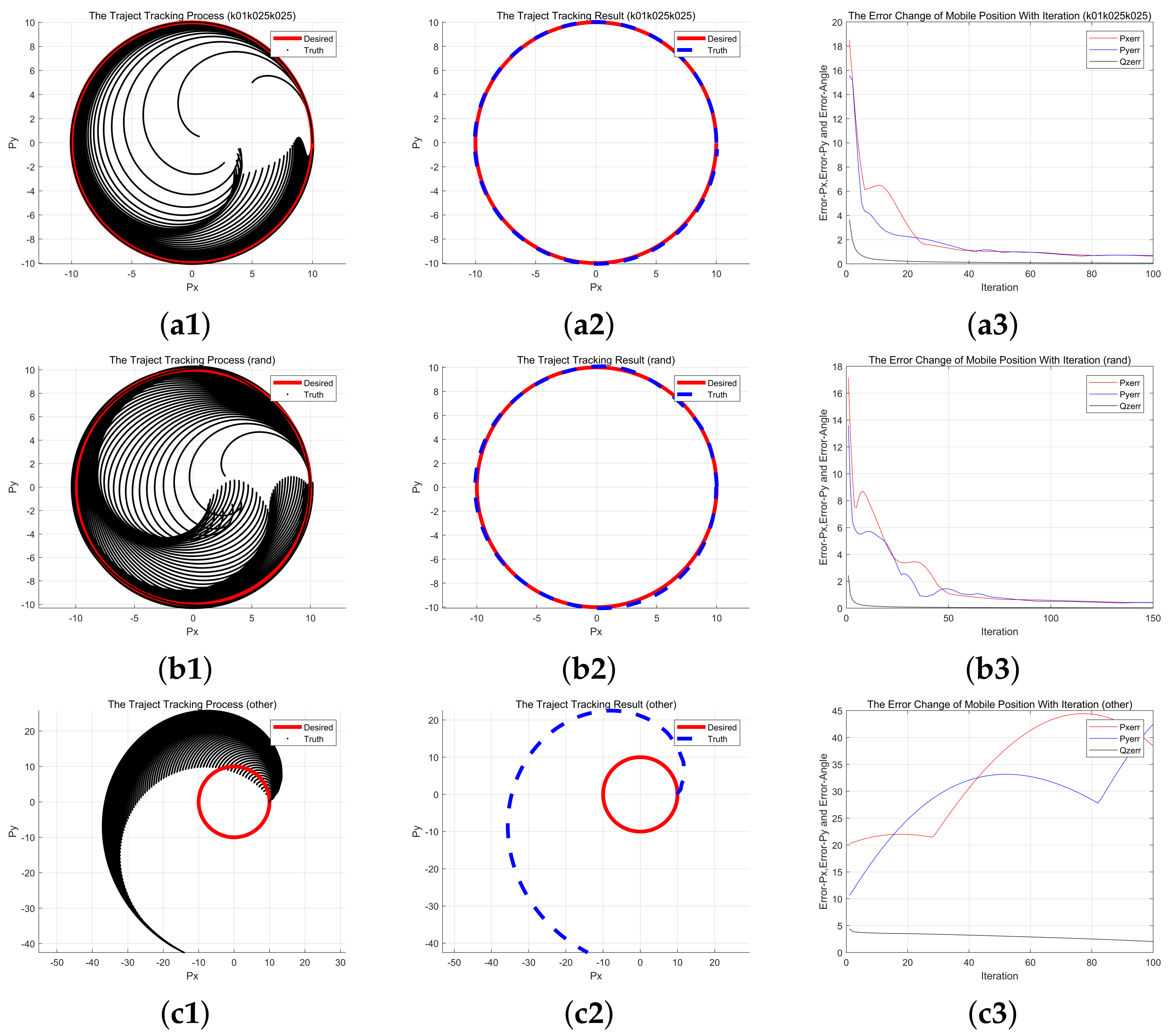
4.1.2. Performance Test of Hybrid Controller with Initial Error

The above tasks were simulated without the initial error; however, the initial position of the mobile platform maybe not completely coincide with the starting of the given trajectory during actual movement. To test the novel-type controller in the initial error state, we effectively compared the previous control law and controller against the circular trajectory’s initial error. We assumed the initial position and posture of the mobile platform are expressed as $(9,0,\pi /2)$, which does not coincide with the initial position of the trajectory in this task. The specific controllers were as follows:

Situation 2: There is an uncompensated control law with a speed constraint, which can be expressed explicitly as follows:

$$\begin{array}{c}{L}_1^{s2}\left(k\right)=0.5·L_1\left(k\right);L_2^{s2}\left(k\right)=0.25·L_1\left(k\right);L_3^{s2}\left(k\right)=0.25·L_1\left(k\right);\end{array}$$

(46)

Situation 3: The iterative learning controller (21) directly controls the rotation speed of the two wheels to solve the trajectory tracking problem, which can be expressed as follows:

$$\begin{array}{c}{u}_{i+1}\left(k\right)=u_i\left(k\right)+L_1\left(k\right)e_i(k+1)+e^{-k·d_t}\theta \left(k\right)L_1\left(k\right)e_i\left(0\right)\hfill \\ \theta \left(k\right)=\left\{\begin{array}{cc}\frac{2}{d_k\ast h}(1-\frac{k}{h}),& \left(0\le k\le h\right)\\ 0,& \left(h<k\le n\right)\end{array}\right.\hfill \end{array}$$

(47)

where $L_1^{s2}\left(k\right)$ is the gain of the controller, which can be expressed as $L_1^{s2}\left(k\right)=0.5·L_1\left(k\right)$; the coefficient of h was chosen as 200; and the corresponding trajectory tracking effect was obtained, as shown in Figure 4.

To illustrate the adaptability of the novel-type controller, we also tested the novel-type controller on other trajectories with initial errors. For example, the initial position and posture of the robot in the combination trajectory of arc and straight task is defined as $(4,0,\pi /2)$, the initial position and posture of the robot in the cardioid-like trajectory task is defined as $(2,0,14\pi /15)$, and the initial position and posture of the robot in the spiral-like trajectory task is defined as $(2.5,0,31\pi /30)$. Using the novel-type controller with a speed constraint, the following experimental results were obtained, as shown in Figure 5.

Comparing the above experimental results, we found the following:

(1)

Without the initial error compensation in Figure 4a1–a3, the control law (17) can achieve closed-loop motion, but the actual trajectory has a relatively fixed deviation from the given trajectory. Therefore, the previous controller cannot control the tracking of the various trajectories with the initial error.

(2)

With the initial error compensation in Figure 4a2,a3,b2,b3, the control law (21) can effectively achieve the circular trajectory tracking with initial error. Additionally, the controller with a velocity constraint must meet the actual physical limitations of the mobile platform.

(3)

According to various trajectory tracking results with initial error in Figure 5, the error compensation controller designed in this paper has good adaptability to various trajectories.

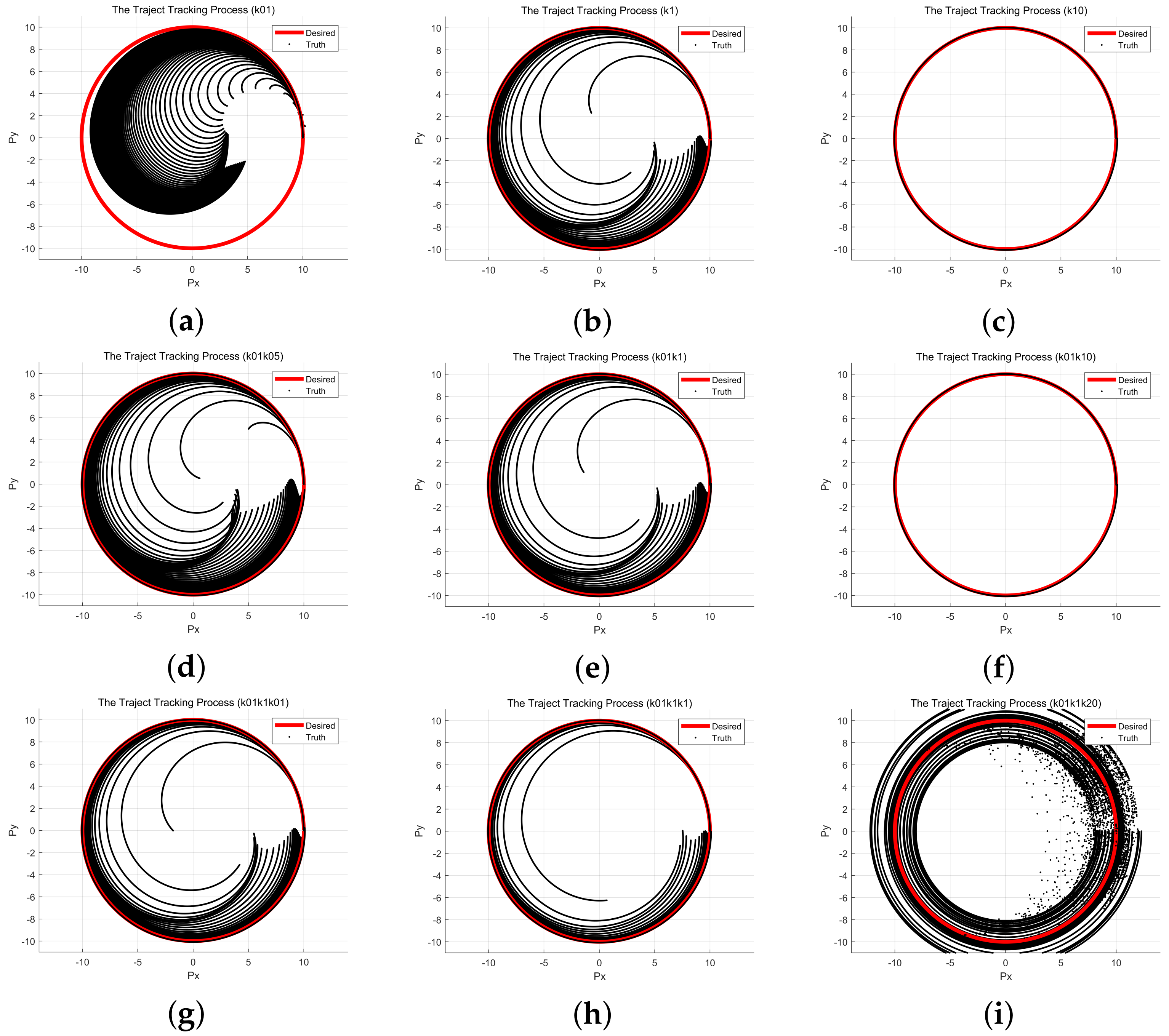
4.2. The Influence of Various Parameters

4.2.1. The Influence of the Control Coefficients and the Error Signals

To study the influence of the error signals and the control coefficients on the trajectory tracking problem, we selected the circular path as the research task for the trajectory tracking with the mobile platform. In the second task, the modified iterative learning control law was selected as the basic controller, and different error signals and the control coefficients were taken as variable parameters. The specific controller settings were as follows:

Situation 4: The $e_i(k+1)$ only uses as the feedback error signal, and the control law (17) is selected as the basic controller. The corresponding gain parameters are described as follows:

$$\begin{array}{c}{L}_1^{s4a}\left(k\right)=0.1·L_1\left(k\right);\hfill \\ L_1^{s4b}\left(k\right)=1.0·L_1\left(k\right);\hfill \\ L_1^{s4c}\left(k\right)=10·L_1\left(k\right);\hfill \end{array}$$

(48)

Situation 5: The $e_i(k+1)$ and $e_{i+1}\left(k\right)$ are used as the feedback error signal, and the control law (17) is selected as the basic controller. The corresponding gain parameters are specifically expressed as follows:

$$\begin{array}{c}{L}_1^{s5a}\left(k\right)=0.1·L_1\left(k\right);L_2^{s5a}\left(k\right)=0.5·L_1\left(k\right);\hfill \\ L_1^{s5b}\left(k\right)=0.1·L_1\left(k\right);L_2^{s5b}\left(k\right)=1.0·L_1\left(k\right);\hfill \\ L_1^{s5c}\left(k\right)=0.1·L_1\left(k\right);L_2^{s5c}\left(k\right)=10·L_1\left(k\right);\hfill \end{array}$$

(49)

Situation 6: The feedback error signal includes $e_i(k+1)$, $e_{i+1}\left(k\right)$, and $e_{i+1}(k-1)$ and the control law (17) is selected as the basic controller. The corresponding gain parameters are specifically expressed as follows:

$$\begin{array}{c}{L}_1^{s6a}\left(k\right)=0.1·L_1\left(k\right);L_2^{s6a}\left(k\right)=1·L_1\left(k\right);L_3^{s6a}\left(k\right)=0.1·L_1\left(k\right);\hfill \\ L_1^{s6b}\left(k\right)=0.1·L_1\left(k\right);L_2^{s6b}\left(k\right)=1·L_1\left(k\right);L_3^{s6b}\left(k\right)=1.0·L_1\left(k\right);\hfill \\ L_1^{s6c}\left(k\right)=0.1·L_1\left(k\right);L_2^{s6c}\left(k\right)=1·L_1\left(k\right);L_3^{s6c}\left(k\right)=20·L_1\left(k\right);\hfill \end{array}$$

(50)

By selecting different controller coefficients and different error parameters, we obtained different dynamic iterative trajectory graphics and the final trajectory result of the mobile platform with 100 iterations, which are shown in Figure 6. To determine the influence of the control coefficient and the error parameter, we compared the various dynamic iterative trajectory graphics, as shown in Figure 6.

(1) Comparing a, b, and c in Figure 6 with different controller coefficients, the number of the iterations required for trajectory tracking can be continuously reduced by increasing the control coefficient within a reasonable range (0.1 to 10). However, if the control coefficient is too small, the controller cannot effectively track the trajectory in a shorter time; if the value of the control coefficient is too large (>20), the controller cannot effectively track the given trajectory caused by increasing the error. Therefore, the system may be unstable.

(2) Comparing a, d, e, g, and h in Figure 6 with different error parameters, if the error at $(k+1)$ time in the current iteration remains unchanged, the other error parameters can compensate for the error parameter to improve the convergence speed of the new-type controller. The tracking performance may be improved by increasing the other error parameter.

(3) Comparing a, d, e, g, and h in Figure 6 with different error parameters and different controller coefficients, increasing the control coefficients of each error parameter can reduce the number of iterations required for the trajectory tracking by the mobile platform; however, the control coefficients of each error parameter still affect the stability of the system.

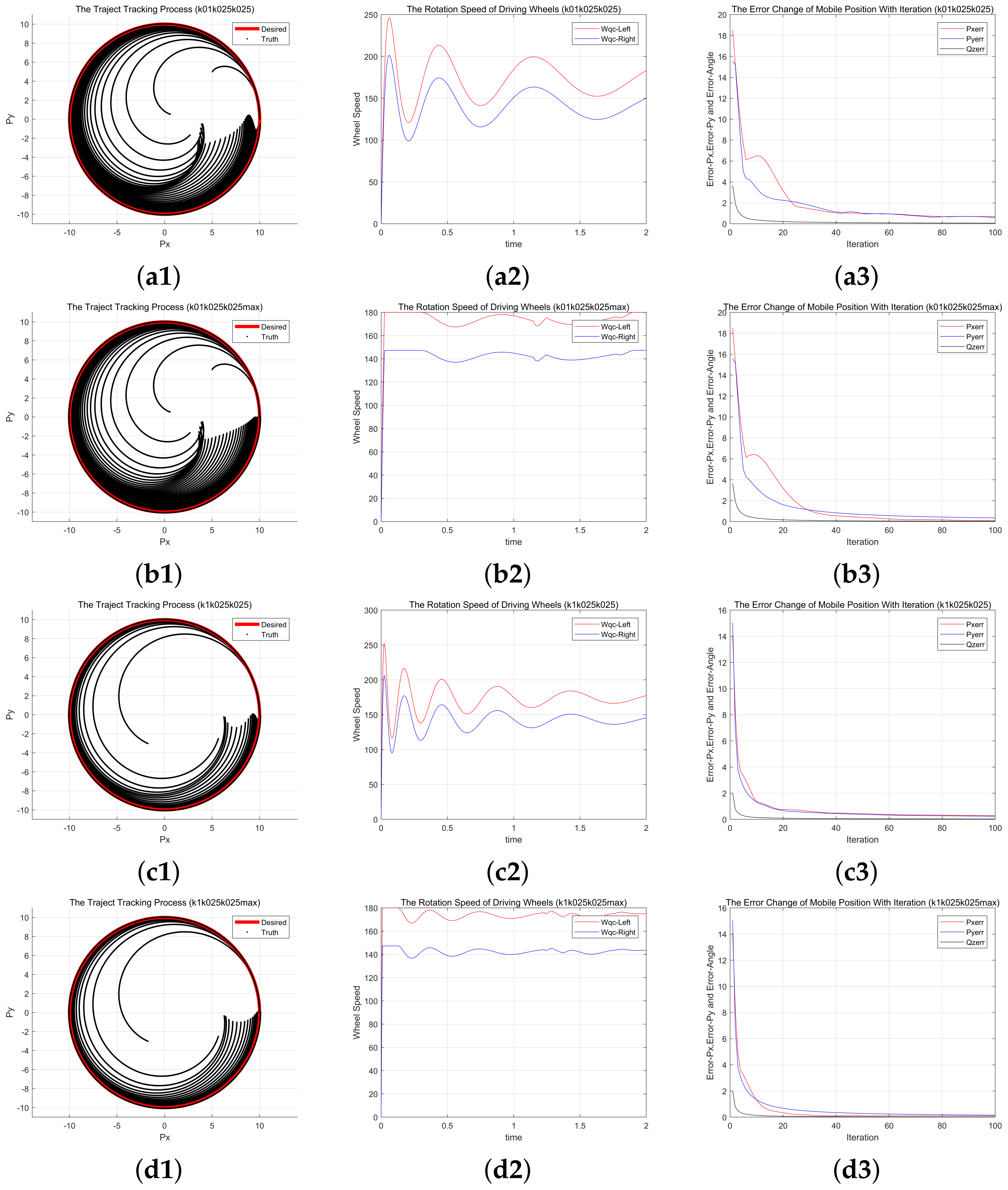
4.2.2. The Influence of the Physical Speed Limitation

The rotation speed of the driving wheel has physical limitations. However, previous studies did not analyze the influence of the speed constraint on the actual trajectory tracking process. Therefore, we deliberately added the speed constraint to the novel-type iterative learning controller to study the impact of the physical speed limitation on the trajectory tracking process. The specific controllers were as follows:

Situation 7: Hybrid iterative learning controller without speed limitation:

$$\begin{array}{c}{L}_1^{s7}\left(k\right)=0.1·L_1\left(k\right);L_2^{s7}\left(k\right)=0.25·L_1\left(k\right);L_3^{s7}\left(k\right)=0.25·L_1\left(k\right);\end{array}$$

(51)

Situation 8: Hybrid iterative learning controller with speed limitation:

$$\left\{\begin{array}{c}{L}_1^{s8}\left(k\right)=0.1·L_1\left(k\right);L_2^{s8}\left(k\right)=0.25·L_1\left(k\right);L_3^{s8}\left(k\right)=0.25·L_1\left(k\right);\\ u_{cr}\left(k\right)<u_{max},ucl\left(k\right)<u_{max}\end{array}\right.$$

(52)

Situation 9: Hybrid iterative learning controller without speed limitation:

$$\begin{array}{c}{L}_1^{s9}\left(k\right)=1·L_1\left(k\right);L_2^{s9}\left(k\right)=0.25·L_1\left(k\right);L_3^{s9}\left(k\right)=0.25·L_1\left(k\right);\end{array}$$

(53)

Situation 10: Hybrid iterative learning controller with speed limitation:

$$\left\{\begin{array}{c}{L}_1^{s10}\left(k\right)=0.5·L_1\left(k\right);L_2^{s10}\left(k\right)=0.25·L_1\left(k\right);L_3^{s10}\left(k\right)=0.25·L_1\left(k\right)\\ u_{cr}\left(k\right)<u_{max},u_{cl}\left(k\right)<u_{max}\end{array}\right.$$

(54)

We used the above controller law to describe the tracking result and error of the specified trajectory. Comparing the above controllers, we found the following:

(1)

Comparing Figure 7a2,c2, the speed solved by the single controller does not meet the physical limitations; however, adding the speed constraint to the controller can meet the physical limitations of the mobile platform.

(2)

Comparing Figure 7a3,b3 or Figure 7c3,d3, the controller with a velocity limitation can reduce the number of system iterations required and improve the convergence speed of the system.

(3)

Comparing Figure 7a2,a3,b2,b3 or Figure 7c2,c3,d2,d3, it can be found that the control signal is not smooth with the speed constraint since the control speed at the next moment can be reached considering the speed limitation. However, the velocity limitation can reduce the tracking error to significantly enhance the performance of the controller.

Figure 7. Circular trajectory tracking results of the mobile platform using the HILC controller with a speed limit. (a1) Path change tracking using HILC law (51). (a2) Final speed of the two-wheels tracking using HILC law (51). (a3) Maximum tracking error change tracking using HILC law (51). (b1) Path change tracking using HILC law (52). (b2) Final speed of the two-wheels tracking using HILC law (52). (b3) Maximum tracking error change tracking using HILC law (52). (c1) Path change tracking using HILC law (53). (c2) Final speed of the two-wheels tracking using HILC law (53). (c3) Maximum tracking error change tracking using ILC law (53). (d1) Path change in tracking using HILC law (54). (d2) Final speed of the two-wheels tracking using HILC law (54). (d3) Maximum tracking error change tracking using HILC law (54).

Figure 7. Circular trajectory tracking results of the mobile platform using the HILC controller with a speed limit. (a1) Path change tracking using HILC law (51). (a2) Final speed of the two-wheels tracking using HILC law (51). (a3) Maximum tracking error change tracking using HILC law (51). (b1) Path change tracking using HILC law (52). (b2) Final speed of the two-wheels tracking using HILC law (52). (b3) Maximum tracking error change tracking using HILC law (52). (c1) Path change tracking using HILC law (53). (c2) Final speed of the two-wheels tracking using HILC law (53). (c3) Maximum tracking error change tracking using ILC law (53). (d1) Path change in tracking using HILC law (54). (d2) Final speed of the two-wheels tracking using HILC law (54). (d3) Maximum tracking error change tracking using HILC law (54).

4.2.3. The Influence of Basic Structure Parameters

To study the influence of the actual structure parameters of the mobile platform on the controller, we compared the controller with the system parameters to that without the system parameters. The specific parameters were as follows:

Situation 11: The novel hybrid controller without error in the parameters of the mobile platform:

$$\begin{array}{c}{L}_1^{s11}\left(k\right)=0.10·L_1\left(k\right);L_2^{s11}\left(k\right)=0.25·L_1\left(k\right);L_3^{s11}\left(k\right)=0.25·L_1\left(k\right);\hfill \end{array}$$

(55)

Situation 12: The novel hybrid controller with error in the parameters of the mobile platform:

$$\begin{array}{cc}\hfill & L_1^{s12}\left(k\right)=\left[\begin{array}{c}\begin{array}{ccc}cos\left(q\right)& sin\left(q\right)& 1\end{array}\\ \begin{array}{ccc}cos\left(q\right)& sin\left(q\right)& -1\end{array}\end{array}\right];\\ \hfill & L_2^{s12}\left(k\right)=0.5·L_1^{s12}\left(k\right);L_3^{s12}\left(k\right)=0.5·L_1^{s12}\left(k\right);\end{array}$$

(56)

Situation 13: The other controller without the control matrix parameters of mobile platforms:

$$\begin{array}{cc}\hfill & L_1^{s13}\left(k\right)=0.1\left[\begin{array}{c}\begin{array}{ccc}0.5& 0.2& B_{rs}/R_{rs}\end{array}\\ \begin{array}{ccc}cos\left(q\right)& sin\left(q\right)& -B_{rs}/R_{rs}\end{array}\end{array}\right];\\ \hfill & L_2^{s13}\left(k\right)=2.5·L_1^{s13}\left(k\right);L_3^{s13}\left(k\right)=2.5·L_1^{s13}\left(k\right);\end{array}$$

(57)

By selecting different Iterative learning controllers, we obtained the different dynamic iterative trajectory graphics and the final trajectory result of the mobile platform, as shown in Figure 8.

(1) Comparing Figure 8a1–a3,b1–b3, the controller without the basic system parameters can still track the circular trajectory, which proves that the iterative controller designed in this article does not depend on the actual parameters.

(2) Comparing Figure 8b1–b3,c1–c3, the designed controller cannot effectively track the given trajectory when the gain matrix $L_1\left(k\right)$ does not conform to the movement characteristics of mobile platforms,.

5. Conclusions

In this study, a new kinematic model of the mobile platform was designed to achieve trajectory tracking by directly controlling the rotation speed of the driving wheels, and the model considers the actual structure and physical constraints of the mobile robot. Different from the typical iterative learning controller of mobile robots, the hybrid controller can directly select the rotation speed of the wheels as the control signal and consider the actual physical constraints of the system.

We theoretically proved the basic performance of the controller, and designed various simulation experiments to analyze the influence of different parameters on the trajectory tracking task, including a speed constraint, the control coefficient, the different error parameters, basic physical parameters, and initial error. Experiments showed that the reference trajectories with or without the initial error can be tracked with the designed hybrid controller, and the system control performance was improved by increasing the other types of error signal in the trajectory tracking task without initial error.

In the future, we aim to develop an iterative controller for mobile platforms to achieve dynamic motion control in various complex environments. In the meantime, we will study the iterative learning method to achieve path planning for mobile platforms with physical limitations in complex environments.

References

1. Guo, P.; Liang, Z.; Wang, X.; Zheng, M. Adaptive trajectory tracking of wheeled mobile robot based on fixed-time convergence with uncalibrated camera parameters. ISA Trans. 2020, 99, 1–8. [Google Scholar] [CrossRef] [PubMed]
2. Stančić, I.; Musić, J.; Grujić, T. Gesture recognition system for real-time mobile robot control based on inertial sensors and motion strings. Eng. Appl. Artif. Intell. 2017, 66, 33–48. [Google Scholar] [CrossRef]
3. Zein, Y.; Darwiche, M.; Mokhiamar, O. GPS tracking system for autonomous vehicles. Alexandria Eng. J. 2018, 57, 3127–3137. [Google Scholar] [CrossRef]
4. Chan, R.P.M.; Stol, K.A.; Halkyard, C.R. Review of modelling and control of two-wheeled robots. Annu. Rev. Control. 2013, 37, 89–103. [Google Scholar] [CrossRef]
5. Luo, S.; Wu, S.; Liu, Z.; Guan, H. Wheeled Mobile Robot RBFNN Dynamic Surface Control Based on Disturbance Observer. ISRN Appl. Math. 2014, 2014, 634936. [Google Scholar] [CrossRef] [Green Version]
6. Scaglia, G.; Rosales, A.; Quintero, L.; Mut, V.; Agarwal, R. A linear-interpolation-based controller design for trajectory tracking of mobile robots. Control Eng. Pract. 2010, 18, 318–329. [Google Scholar] [CrossRef]
7. Shojaei, K.; Shahri, A.M.; Tarakameh, A. Adaptive feedback linearizing control of nonholonomic wheeled mobile robots in presence of parametric and nonparametric uncertainties. Robot. Comput. Integr. Manuf. 2011, 27, 194–204. [Google Scholar] [CrossRef]
8. Wu, D.; Cheng, Y.; Du, H.; Zhu, W.; Zhu, M. Finite-time output feedback tracking control for a nonholonomic wheeled mobile robot. Aerosp. Sci. Technol. 2018, 78, 574–579. [Google Scholar] [CrossRef]
9. Alakshendra, V.; Chiddarwar, S.S. Adaptive robust control of Mecanum-wheeled mobile robot with uncertainties. Nonlinear Dyn. 2017, 87, 2147–2169. [Google Scholar] [CrossRef]
10. Begnini, M.; Bertol, D.W.; Martins, N.A. A robust adaptive fuzzy variable structure tracking control for the wheeled mobile robot: Simulation and experimental results. Control Eng. Pract. 2017, 64, 27–43. [Google Scholar] [CrossRef]
11. Fierro, R.; Lewis, F.L. Control of a nonholonomic mobile robot: Backstepping kinematics into dynamics. J. Robot. Syst. 1997, 14, 149–163. [Google Scholar] [CrossRef]
12. He, N.; Qi, L.; Li, R.; Liu, Y. Design of a Model Predictive Trajectory Tracking Controller for Mobile Robot Based on the Event-Triggering Mechanism. Math. Probl. Eng. 2021, 2021, 5573467. [Google Scholar] [CrossRef]
13. Liu, K.; Gong, J.; Chen, S.; Zhang, Y.; Chen, H. Model predictive stabilization control of high-speed autonomous ground vehicles considering the effect of road topography. Appl. Sci. 2018, 8, 5. [Google Scholar] [CrossRef] [Green Version]
14. Matraji, I.; Al-Durra, A.; Haryono, A.; Al-Wahedi, K.; Abou-Khousa, M. Trajectory tracking control of Skid-Steered Mobile Robot based on adaptive Second Order Sliding Mode Control. Control Eng. Pract. 2017, 11, 167–176. [Google Scholar] [CrossRef]
15. Goswami, N.K.; Padhy, P.K. Sliding mode controller design for trajectory tracking of a non-holonomic mobile robot with disturbance. Comput. Electr. Eng. 2018, 72, 307–323. [Google Scholar] [CrossRef]
16. Aouf, A.; Boussaid, L.; Sakly, A. TLBO-Based Adaptive Neurofuzzy Controller for Mobile Robot Navigation in a Strange Environment. Comput. Intell. Neurosci. 2018, 2018, 3145436. [Google Scholar] [CrossRef] [PubMed]
17. Omrane, H.; Masmoudi, M.S.; Masmoudi, M. Fuzzy Logic Based Control for Autonomous Mobile Robot Navigation. Comput. Intell. Neurosci. 2016, 2016, 9548482. [Google Scholar] [CrossRef] [Green Version]
18. Dixon, W.E.; Dawson, D.M.; Zergeroglu, E.; Behal, A. Adaptive tracking control of a wheeled mobile robot via an uncalibrated camera system. IEEE Trans. Syst. Man, Cybern. Part B Cybern. 2001, 31, 341–352. [Google Scholar] [CrossRef] [Green Version]
19. Xin, L.; Wang, Q.; She, J.; Li, Y. Robust adaptive tracking control of wheeled mobile robot. Rob. Auton. Syst. 2016, 78, 36–48. [Google Scholar] [CrossRef]
20. Cui, M.; Sun, D.; Liu, W.; Zhao, M.; Liao, X. Adaptive tracking and obstacle avoidance control for mobile robots with unknown sliding. Int. J. Adv. Robot. Syst. 2012, 9, 1–14. [Google Scholar] [CrossRef]
21. Hoang, N.B.; Kang, H.J. Neural network-based adaptive tracking control of mobile robots in the presence of wheel slip and external disturbance force. Neurocomputing 2016, 188, 12–22. [Google Scholar] [CrossRef]
22. Li, S.; Ding, L.; Gao, H.; Chen, C.; Liu, Z.; Deng, Z. Adaptive neural network tracking control-based reinforcement learning for wheeled mobile robots with skidding and slipping. Neurocomputing 2018, 283, 20–30. [Google Scholar] [CrossRef]
23. Boukens, M.; Boukabou, A.; Chadli, M. Robust adaptive neural network-based trajectory tracking control approach for nonholonomic electrically driven mobile robots. Rob. Auton. Syst. 2017, 92, 30–40. [Google Scholar] [CrossRef]
24. Boudjedir, C.E.; Bouri, M.; Boukhetala, D. Iterative learning control for trajectory tracking of a parallel Delta robot. At-Automatisierungstechnik 2019, 67, 145–156. [Google Scholar] [CrossRef]
25. Dong, J.; He, B.; Zhang, C.; Li, G. Open-Closed-Loop PD Iterative Learning Control with a Variable Forgetting Factor for a Two-Wheeled Self-Balancing Mobile Robot. Complexity 2019, 2019, 5705126. [Google Scholar] [CrossRef] [Green Version]
26. Lu, X.; Fei, J. Velocity Tracking Control of Wheeled Mobile Robots by Iterative Learning Control. Int. J. Adv. Robot. Syst. 2016, 13, 1–10. [Google Scholar] [CrossRef] [Green Version]
27. Son, T.D.; Ahn, H.S.; Moore, K.L. Iterative learning control in optimal tracking problems with specified data points. Automatica 2013, 49, 1465–1472. [Google Scholar] [CrossRef]
28. Li, G. Adaptive iterative learning control for nonlinear systems with unknown control direction. Nanjing Li Gong Daxue Xuebao/J. Nanjing Univ. Sci. Technol. 2015, 39, 2942–2950. [Google Scholar] [CrossRef]
29. Bouakrif, F.; Zasadzinski, M. High order iterative learning control to solve the trajectory tracking problem for robot manipulators using Lyapunov theory. Trans. Inst. Meas. Control 2018, 40, 4105–4114. [Google Scholar] [CrossRef]
30. Bouakrif, F.; Boukhetala, D.; Boudjema, F. Velocity observer-based iterative learning control for robot manipulators. Int. J. Syst. Sci. 2013, 44, 214–222. [Google Scholar] [CrossRef]
31. Ahn, H.S.; Chen, Y.Q.; Moore, K.L. Iterative learning control: Brief survey and categorization. IEEE Trans. Syst. Man Cybern. Part C Appl. Rev. 2007, 37, 1099–1121. [Google Scholar] [CrossRef]
32. Wang, Y.; Gao, F.; Doyle, F.J. Survey on iterative learning control, repetitive control, and run-to-run control. J. Process Control 2009, 19, 1589–1600. [Google Scholar] [CrossRef]
33. Kang, M.K.; Lee, J.S.; Han, K.L. Kinematic path tracking of mobile robot using iterative learning control. J. Robot. Syst. 2005, 22, 111–121. [Google Scholar] [CrossRef]
34. Han, K.L.; Lee, J.S. Iterative path tracking of an omni-directional mobile robot. Adv. Robot. 2011, 25, 1817–1838. [Google Scholar] [CrossRef]
35. Yu, C.; Chen, X. Trajectory tracking of wheeled mobile robot by adopting iterative learning control with predictive, current, and past learning items. Robotica 2015, 33, 1393–1414. [Google Scholar] [CrossRef]
36. Wang, H.; Dong, J.; Wang, Y. Discrete PID-Type Iterative Learning Control for Mobile Robot. J. Control Sci. Eng. 2016, 2016, 2320746. [Google Scholar] [CrossRef]
37. Wang, H.; Dong, J.; Wang, Y. Research on Open-Closed-Loop Iterative Learning Control with Variable Forgetting Factor of Mobile Robots. Discret. Dyn. Nat. Soc. 2016, 2016, 6452179. [Google Scholar] [CrossRef] [Green Version]
38. Zhao, Y.; Zhou, F.; Li, Y.; Wang, Y. A novel iterative learning path-tracking control for nonholonomic mobile robots against initial shifts. Int. J. Adv. Robot. Syst. 2017, 14. [Google Scholar] [CrossRef] [Green Version]
Figure 1. The basic parameters of the mobile platform. (a) The top view and corresponding parameters. (b) The side view and corresponding parameters.
Applsci 11 08181 g001
Figure 2. Framework for the hybrid iterative learning controller (“+” represents the input, “−” represents the feedback).
Applsci 11 08181 g002
Figure 3. Typical trajectory tracking results of the mobile platform using the P−type iterative learning controller. (a1) Path change in single circular trajectory. (a2) Final path in single circular trajectory. (a3) Maximum tracking error change in single circular trajectory. (b1) Path change in mixed arc and line closed trajectory. (b2) Final path in mixed arc and line closed trajectory. (b3) Maximum tracking error change in mixed arc and line closed trajectory. (c1) Path change in cardioid−like trajectory. (c2) Final path in cardioid−like trajectory. (c3) Maximum tracking error change in cardioid−like trajectory. (d1) Path change in spiral−like trajectory. (d2) Final path in spiral−like trajectory. (d3) Maximum tracking error change in spiral−like trajectory.
Applsci 11 08181 g003
Figure 4. Circular trajectory tracking results of the mobile platform using the HILC controller with initial error. (a1) Path change tracking using HILC law (46). (a2) Final path tracking using HILC law (46). (a3) Average tracking error change using HILC law (46). (b1) Path change tracking using HILC law (47). (b2) Final path tracking using HILC law (47). (b3) Average tracking error change using HILC law (47).
Applsci 11 08181 g004
Figure 5. Other typical trajectories tracking results of mobile platform using the HILC law (47) with Initial error. (a1) Path change of mixed the arc and line closed trajectory tracking using HILC law (47). (a2) Final path of mixed the arc and line closed trajectory tracking using HILC law (47). (a3) Average error of the arc and line mixed closed trajectory tracking using HILC law (47). (b1) Path change of the cardioid-like trajectory tracking using HILC law (47). (b2) Final path of the cardioid-like trajectory tracking using HILC law (47). (b3) Average error of the cardioid-like trajectory tracking using HILC law (47). (c1) Path change of the spiral-like trajectory tracking using HILC law (47). (c2) Final path of the spiral-like trajectory tracking using HILC law (47). (c3) Average error of the spiral-like trajectory tracking using HILC law (47).
Applsci 11 08181 g005
Figure 6. Circular trajectory tracking results of the mobile platform using the HILC controller with different parameters. (a) Using the HILC law with k 1 = 0.1 . (b) Using the HILC law with k 1 = 1 . (c) Using the HILC law with k 1 = 10 . (d) Using the HILC law with k 1 = 0.1 , k 2 = 0.5 . (e) Using the HILC law with k 1 = 0.1 , k 2 = 1 . (f) Using the HILC law with k 1 = 0.1 , k 2 = 10 . (g) Using the HILC law with k 1 = 0.1 , k 2 = 1 , k 3 = 0.1 . (h) Using the HILC law with k 1 = 0.1 , k 2 = 1 , k 3 = 1 . (i) Using the HILC law with k 1 = 0.1 , k 2 = 1 , k 3 = 20 .
Applsci 11 08181 g006
Figure 8. Circular trajectory tracking results of the mobile platform using the HILC controller with different structure parameters. (a1) Path change tracking using HILC law (55). (a2) Final path tracking using HILC law (55). (a3) Maximum tracking error change using HILC law (55). (b1) Path change tracking using HILC law (56). (b2) Final path tracking using HILC law (56). (b3) Maximum tracking error change using HILC law (56). (c1) Path change tracking using HILC law (57). (c2) Final path tracking using HILC law (57). (c3) Maximum tracking error change using HILC law (57).
Applsci 11 08181 g008
Publisher’s Note: MDPI stays neutral with regard to jurisdictional claims in published maps and institutional affiliations.