Article

A Novel Principal Component Analysis Integrating Long Short-Term Memory Network and Its Application in Productivity Prediction of Cutter Suction Dredgers

School of Energy and Power Engineering, Wuhan University of Technology, Wuhan 430063, China
*
Author to whom correspondence should be addressed.
Appl. Sci. 2021, 11(17), 8159; https://doi.org/10.3390/app11178159
Submission received: 22 July 2021 / Revised: 27 August 2021 / Accepted: 30 August 2021 / Published: 2 September 2021
(This article belongs to the Special Issue Sensors and Measurement Systems for Marine Engineering Applications)

Abstract

:
Dredging is a basic construction for waterway improvement, harbor basin maintenance, land reclamation, environmental protection dredging, and deep-sea mining. The dredging process of cutter suction dredgers is so complex that the operational data show strong characteristics of dynamic, nonlinearity, and time delay, which make it difficult to predict the productivity accurately via basic principles models. In this paper, we propose a novel integrating PCA-LSTM model to improve the productivity prediction of cutter suction dredger. Firstly, multiple variables are reduced in dimension and selected by PCA method based on the working mechanism of cutter suction dredger. Then the productivity is predicted via mud concentration in long short-term memory network with relevant operational time-series data. Finally, the proposed method is successfully applied to an actual case study in China. Also, it performs well in the cross-validation and comparative study for several important characteristics: (i) it involves the operational parameters based on the mechanism analysis; and (ii) it is a deep-learning-based approach that can deal with operation series data with a special memory mechanism. This study provides a heuristic idea for integrating the data-driven method and supervision of human knowledge for application in practical engineering.

1. Introduction

Marine-based transportation has always played a critical role in the national economics of China [1], while rivers may suffer from sediment accumulation that obstructs riverways and reduces the carrying activity [2,3]. Cutter suction dredgers are common and useful machines that can remove the mud deposited at the bottom of water and keep transportation routes in good condition [4]. Dredging productivity is one of the most important indexes to evaluate the dredging performance, which is affected by many factors such as soil properties, the power of the pump, the cutter structural parameters, and so on [5]. The process of sand being cut into a mixture of mud and water by a rotating cutter is very complicated. Most of the parameters are dynamically influenced by the uncertain working environment and human operation [6]. Due to the limitations of dredging technology, there are indeed some obstacles for parameters monitoring and real-time prediction, which is a challenge for constructing digital models to describe this process and dredging productivity accurately [7].
Due to the developed sensor technology, more operational data have been gained for analyzing dredging performance. In the literature review, machine learning methods were recently adopted to model the complex and dynamical construction process of CSD (cutter suction dredger) for their excellent learning and mining ability [8]. Generally, the learning-based prediction models can be mainly divided into two main types based on the depth of structure: shallow learning models and deep learning models [9]. The shallow learning methods mainly cover neural-network-based methods such as RBF (radial basis function), ELMs (extreme learning machines), and SVM (support vector machine). As traditional learning models used in productivity prediction, Wang et al. adopted an RBF neural network to deal with the different working conditions and established an accurate nonlinear mathematical model for the instantaneous output prediction with control variables [10]. Guan et al. developed the model of cutter operation parameters using improved ELMs to simulate and predict the productivity distribution in actual construction [11]. Yang et al. predicted the cutter suction dredger production with a double hidden layer BP neural network [12].
The prediction methods on deep learning mainly include: DNN (deep neural network), DBN (deep belief network), CNN (convolutional neural network network), and RNN (recurrent neural network network). DNNs are adopted through multiple auto-encoder (AE) or denoising auto-encoder (DAE) stacking networks, wherein high-dimensional input data are extracted from classless data as the distribution of the original data is represented by deep learning neural networks [13]. Wang et al. developed DNN models for production forecasting wherein the data-driven method was well used to deal with hydraulic fractures and intrinsic complexity [14]. DNN architecture transfers sigmoid function to ReLu and maxout with the purpose of overcoming gradient disappearance, but requires small batch training, which leads to over-fitting and local optimal solution problems. DBN is also a deep network that is stacked with multiple Restricted Boltzman Machines (RBMs) and a classification layer or regression layer. Xu et al. designed a DBN-based model to approximate the function type coefficients of a state-dependent autoregressive model in nonlinear system and realize predictive control [15]. Hu et al. adopted DBN to extract deep hidden features behind the monitoring signals and predict the bearing remaining useful life [16]. Researchers have improved DBN by combining a feed-forward neural network (FNN) to make prediction more accurate [17]. Zhang proposed a multi-target DBN collection method in which the output of multiple DBNs has a certain weight that reveals the final output of the network set; this method performed well on NASA aero-engine data [18]. Furthermore, convolutional neural networks (CNNs) are greatly developed with the excellent characteristics of parameter sharing and spatial pooling, which make it more advantageous in computing speed and accuracy [19]. However, all these ML methods have a limitation in situations that involve a time-series input.
Then recurrent neural networks (RNNs) are proposed with adding a twist where the output from previous time step is fed as input to the current step. The most important feature of RNN is that the hidden state can remember all information calculated from the previous sequence [20]. Thus, it can generate output through prior input (the past memory) and learning in training. It is common to complete the parameter learning of recurrent neural networks by learning over back-propagation, wherein the error is passed forward step by step in the reverse order of time. In [21], a learning-based method is applied to improve the RNN training process while the number of prediction time-steps increases. However, RNNs still suffer from the long-term dependencies, and long short-term memory (LSTM) fills the gap by setting a gate control unit that can choose and keep some useful information in the long-term sequential data. Being different from the traditional RNN, the model is trained by both the stored information of last time step and new input of the current moment, which enhances the prediction accuracy and stability greatly [22].
However, for the practical application in CSD, it is equally significant to analyze the interrelated influencing factors as the productivity prediction. LSTM lacks effective processing for high-dimensional characteristics of large-scale data; it should be used integrating with other methods. Principal component analysis (PCA) is one of the most widely used algorithms for feature reduction, which reconstructs the main k-dimensional feature based on the original n-dimensional feature by deep learning. While PCA is a pure data-driven method that cannot consider the casual relationship and correlation between variables, the procedure of variable analysis based on a working mechanism and human experience is necessary. Yang et al. described a HEPCA model, which made variables supplement based on expert knowledge after the PCA process and generate a more accurate input for the predictive model [23].
Therefore, combining the advantages and characteristics of the different methods described above, this paper presents the long short-term memory integrating principal component analysis model (PCA-LSTM) to predict productivity using the monitoring sensors data. The PCA-LSTM is strutted into four phases. In the first phase, monitoring sensors are analyzed to select related variables according to the working mechanism and knowledge. In the second phase, PCA method is applied to extract the deep feature from the high-dimension dataset and to obtain the correlation of variables. In the third phase, a prediction model is built and trained by the LSTM network. Finally, cross validation and comparative analysis are conducted with a generated model from “Chang Shi 10” in China.

2. Preliminaries

In this section, the related preliminaries regarding PCA and LSTM will be introduced briefly on the basis of the practical application in this study.

2.1. Principal Components Analysis (PCA)

PCA is an important technique that can transform multiple variables into a few main components (comprehensive variables) by means of dimensional reduction, increasing interpretability while minimizing information loss [24]. These main components are usually expressed as linear combinations of the original variables, which can represent most of the information of the whole dataset.
For original data X = x 1 , x 2 , , x i , , x n and X k n , we can get the covariance matrix C x :
C x = E [ ( X E [ X ] ) ( X E [ X ] ) T ]
After centralizing the data, the mean function E [ X ] is zero and:
C x = 1 n X X T
Assuming that there is a matrix P ( P k k ), through which we can transform the original sample data matrix X into a dimensionality-reduced matrix Y ( Y k n ):
Y = P X
Then the original data dimension is successfully reduced from k to k , wherein the first k principal components can explain most of the variance.
For matrix Y , its covariance matrix can be expressed through original matrix X as:
C y = 1 n Y Y T = 1 n ( P X ) ( P X ) T = 1 n P X X T P T = P 1 n X X T P T = P C x P T
It is obvious from Equation (4) that C x is guaranteed to be a non-negative definite matrix and thus is diagonalizable by some unitary matrix. Then the objective optimization is transformed to find an orthonormal transformation matrix P . Normally, we can use eigenvalue decomposition or singular value decomposition to solve the matrix P , and the first k -dimensional new features corresponding to k eigenvalues can represent the whole data best.

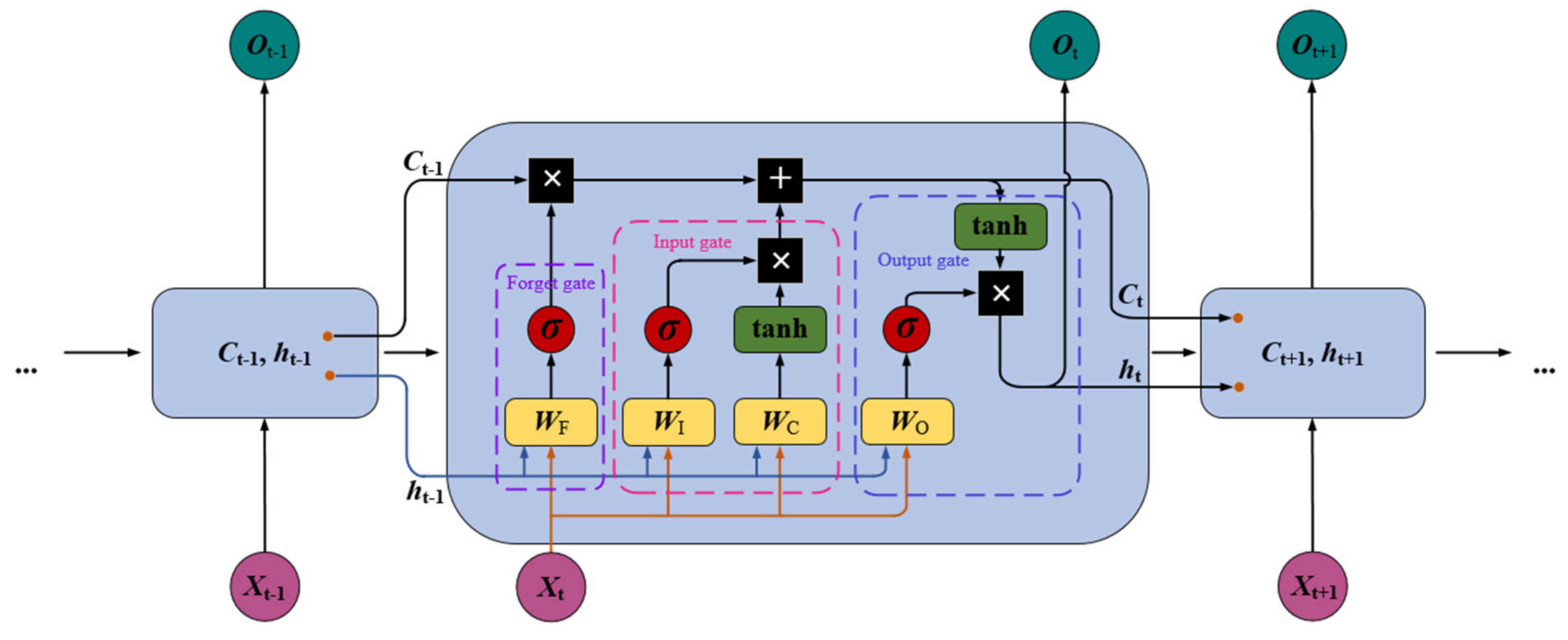
2.2. Long Short-Term Memory Network (LSTM)

In this paper, an integrating model of long short-term memory network based on principal components analysis (PCA-LSTM) is explored to analyze the operational time-series data generated from the dredging process. The proposed model is developed on the basis of long short-term memory network (LSTM), which is a special form of recurrent neural networks (RNN) that can address long-distance dependencies and delay in time-series modeling.
The LSTM architecture was firstly proposed by Sepp Hochreiter and Jürgen Schmidhuber in 1997 [25]. There is a special memory cell unit added to the original hidden layer in classic RNN architecture. The cell state is controlled by three gates: Input gate I t , Forget gate F t , and Output gate O t , as shown in Figure 1.
The forget gate F t decides which information needs to be kept and which can be forgotten. The information consists of the current input X t and previous hidden state/short-term memory h t 1 .
F t = σ ( W F o r e g e t [ h t 1 , X t ] ) + b i a s F o r g e t
For every time step, the sigmoid function generates values between 0 and 1 that indicate whether the old information is necessary. 0 denotes forget, and 1 means keep. W F o r g e t is the weight matrix between forget gate and input gate. b i a s F o r g e t is the connection bias.
The input gate decides what should be stored in the long-term memory in the new information. It works with the current input X t and previous short memory h t 1 through two layers. In the first layer, the short-term memory and current input is passed through a sigmoid function that values from 0 (not important) to 1 (important):
i t = σ ( W I n p u t [ h t 1 , X t ] ) + b i a s I n p u t
where W I n p u t is the weight matrix of sigmoid operator between input gate and output gate. b i a s I n p u t is the bias vector.
The second layer uses the tanh function to regulate the network. The tanh operator creates a vector C ˜ t with all the possible values between −1 and 1:
C ˜ t = tanh ( W C e l l [ h t 1 , X t ] ) + b i a s C e l l
where W c e l l is the weight matrix of tanh operator between cell state information and network output. b i a s C e l l is the bias vector.
With these two layers input, the cell state updates a new cell state (long-term memory):
C t = F t C t 1 + i t C ˜ t
where is the Hadamard product.
When it comes to the output gate, the current input X t , the previous short-term memory h t 1 , and the newly obtained cell state C t determine the new short-term memory (hidden state) that will be passed on to the cell in the next time step.
O t = σ ( W o u t p u t [ h t 1 , X t ] ) + b i a s o u t p u t
h t = O t tanh ( C t )
W o u t p u t is the weight matrix of the output gate. This hidden state is used for prediction. Both new cell state and hidden state are carried over to the next time step.

3. The Proposed PCA-LSTM Model

As described above, the basic knowledge regarding PCA and LSTM networks was introduced to set up the proposed PCA-LSTM model in this section. Considering mechanism and human experience, the PCA procedure will bring about a more accurate variable analysis for the practical multi-sensors system. The time-series data of effective variables are subsequently learned in LSTM network to output the target prediction.

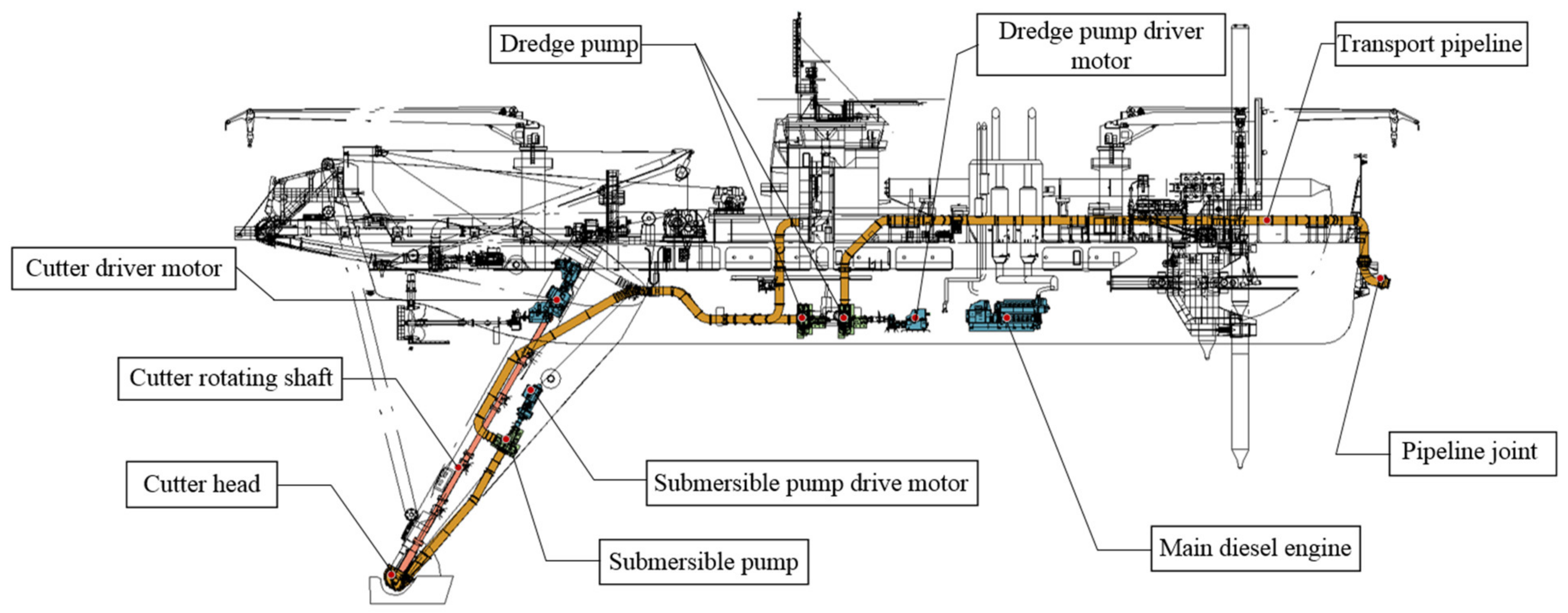
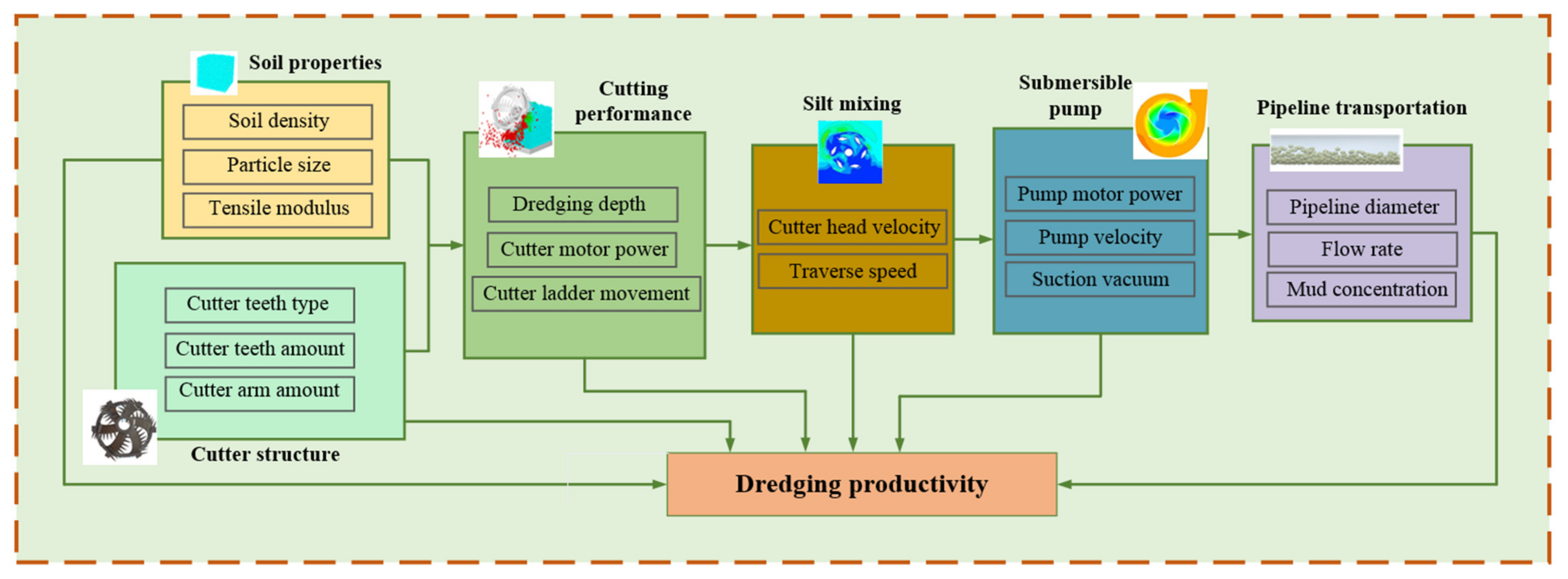
3.1. PCA Based on Mechanism

The traditional PCA was introduced in Section 2.1. Due to the purely data-driven process, historical data is analyzed in PCA without any prior knowledge, which may bring about that some redundancies may be considered despite the causal relationship. Therefore, human experience will be introduced to interfere with the variable selection procedure ahead of PCA, based on the known mechanism.
The monitoring system always contains a broad range of sensors data related to the target object. Some of the data is on control variables, while some of the data is just on display variables that visualize the parameters.
Assuming the sensor system obtains an initial dataset:
X = x 1 , x 2 , , x i m , x i m + 1 , , x i , , x k
where x i represents the i -th sensor equipped in the system.
x i = [ x i 1 , x i 2 , , x i j , , x i n ] T
where x i j represents the j -th data obtained by i -th sensor.
When studying the working mechanism of the target, variables causal relationship will be analyzed and some of the redundant variables will be deleted, as well as some meaningless display parameters. This creates a new sample set:
X = x 1 , x 2 , , x i m , x i , , x k
PCA based on human experience method obtains a hyperplanar representation of all samples through recent reconstruction, realizing the dimension reduction from k to k with the least loss.
The samples are centralized firstly as:
i x i = 0
Then a new coordinate system can be obtained after projection transformation:
W = ( w 1 , w 2 , w i m , w i , , w k )
where w i is the standard orthogonal basis vector.
w i 2 = 1
w i T w j = 0 , ( i j )
If a portion of the coordinate is abandoned, namely the dimension is reduced from k to k ( k < k ), the projection of samples x i in the low-dimensional coordinate system will be:
z i j = ( z i 1 , z i 2 , , z i n )
z i j = w j T x i
where z i j is the j -th coordinate of x i in low-dimensional space; and x i can be reconstructed as:
x ^ i = j = 1 k z i j w j
For the whole training dataset, the distance between original samples x i and the reconstructed samples x ^ i can then be determined as:
i = 1 k j = 1 n z i j w j x i 2 2 = i = 1 k z i T z i 2 i = 1 k z i T W T x i + c o n s t t r ( W T ( i = 1 k x i x i T ) W )
where const is the constant item, and W can be obtained by Equation (15).
Because i = 1 k x i x i T is a covariance matrix, the target distance function can be minimized as:
M i n W   t r W T X X T W s . t . W T W = I
where I is the identity matrix.
With the Langerin multiplier method [26], it can be calculated as:
X X T w i = λ i w i
After eigenvalue decomposition, the eigenvalue λ can be obtained as follows:
λ = { λ 1 , λ 2 , , λ i m , λ i , , λ k )
According to the practical demand, reconstruction threshold μ is set to satisfy the condition:
i = 1 k λ i i = 1 k λ i μ
When the maximum threshold μ is satisfied, the eigenvalues can be obtained in turn:
λ 1 λ 2 λ k
And the eigenvectors corresponding to the first k eigenvalues constitute the PCA solution:
W * = ( w 1 , w 2 , , w i m , w i , , w k )
The variables corresponding to the eigenvectors are:
X = ( x 1 , x 2 , , x i m , x i , , x k )
Based on the variables obtained by PCA procedure above, the correlation matrix can be calculated as:
R = ( r i j ) k k
Then the most positively relevant variables to the target will be proceeded in the subsequent prediction model:
X * * = ( x 1 , x 2 , , x p )

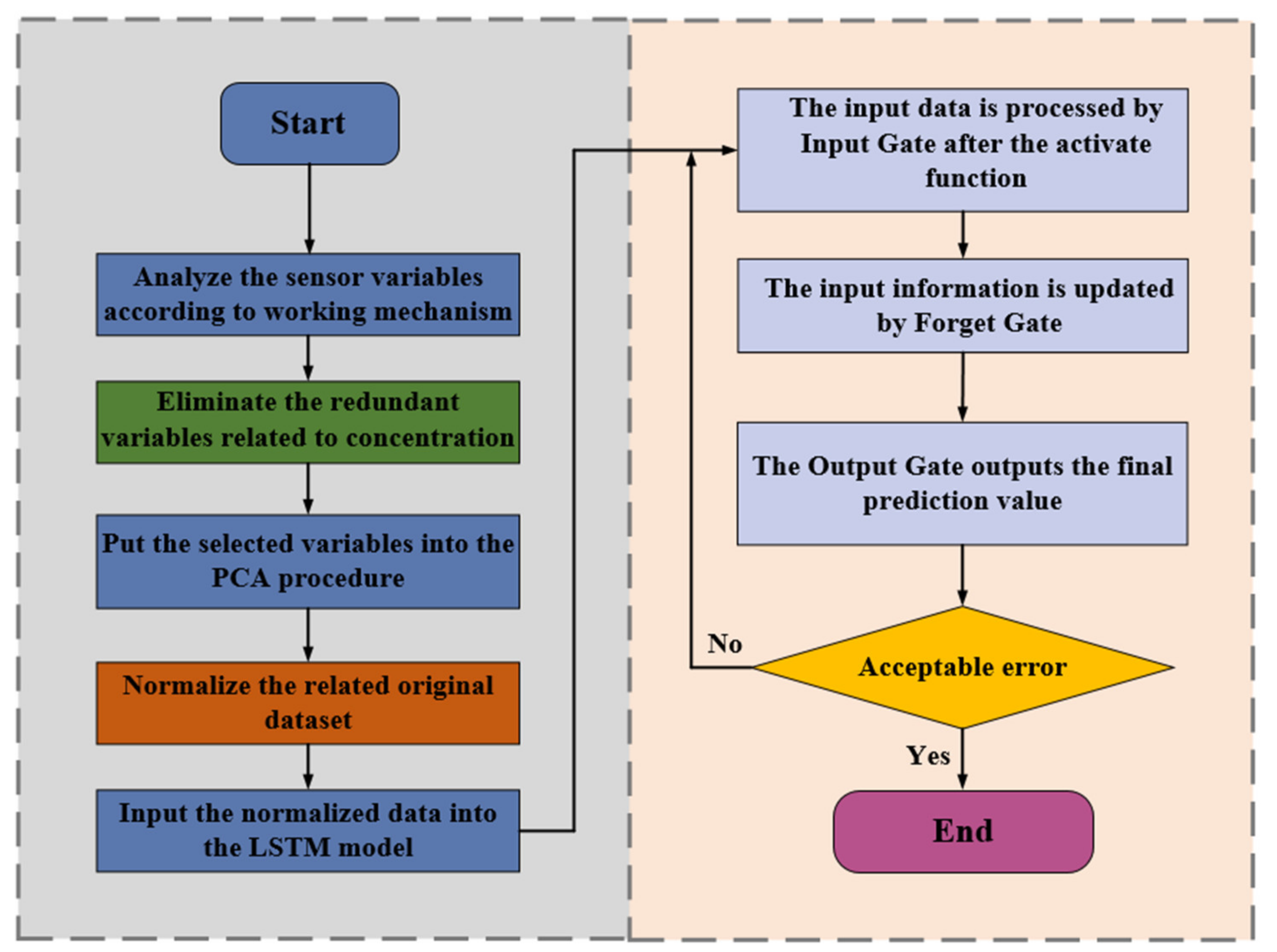
3.2. The Proposed Methodology

The variables most related to the target were obtained by PCA based on human experience that can be used as inputs in the next LSTM network to obtain prediction results. Namely, with current input being X t * * , the current cell state and hidden state are updated as described in Section 2.2.
C t = F t C t 1 + i t C ˜ t = F t C t 1 + i t { tanh ( W C e l l [ h t 1 , X t * * ] ) + b i a s c e l l } = { σ ( W F o r g e t · [ h t 1 , X t * * ] ) + b i a s F o r g e t } C t 1 + { σ ( W I n p u t · [ h t 1 , X t * * ] ) + b i a s I n p u t } { tanh ( W C e l l · [ h t 1 , X t * * ] ) + b i a s C e l l }
h t = O t tanh ( C t ) = { σ ( W o u t p u t · [ h t 1 , X t * * ] ) + b i a s o u t p u t } tanh ( C t )
Based on the new cell state and hidden state, we define gradient δ h ( t ) and δ c ( t ) to calculate the back propagation error layer by layer:
δ h ( t ) = L ( t ) h ( t )
δ c ( t ) = L ( t ) C ( t )
where L ( t ) is the loss function, and at the last sequence index τ , the gradient can be described as follows:
δ h ( τ ) = L ( τ ) O ( τ ) O ( τ ) h ( τ ) = W O u t p u t T ( O ^ ( τ ) O ( τ ) )
δ c ( τ ) = L ( τ ) h ( τ ) h ( τ ) C ( τ ) = δ h ( τ ) O ( τ ) ( 1 tanh 2 ( C ( τ ) ) )
Therefore, for any moment t , δ h ( t + 1 ) and δ c ( t + 1 ) can be obtained, deriving from δ h ( t ) and δ c ( t ) as follows:
δ h ( t ) = L ( t ) O ( t ) O ( t ) h ( t ) + L ( t + 1 ) h ( t + 1 ) h ( t + 1 ) h ( t ) = W O u t p u t T ( O ^ ( t ) O ( t ) ) + W T δ h ( t + 1 ) d i a g ( 1 ( h ( t + 1 ) ) 2 )
where W is the coefficient matrix.
Then the reverse gradient error of δ c ( t ) can be obtained through the gradient error of the current layer returned from h ( t ) and the gradient error of the previous layer δ c ( t ) :
δ c ( t ) = L ( t ) C ( t + 1 ) C ( t + 1 ) C ( t ) + L ( t ) h ( t ) h ( t ) C ( t ) = δ c ( t + 1 ) F ( t + 1 ) + δ h ( t ) O ( t ) ( 1 tanh 2 ( C ( t ) ) )
Then, the gradient of all parameters can be calculated easily using δ h ( t ) and δ c ( t ) , and all the parameters can be updated iteratively with the lowest error.
As mentioned above, the proposed method can be run in terms of Figure 2. It mainly consists of two parts: PCA and LSTM. The variables most related to the target are firstly obtained by PCA based on expert knowledge and used as inputs for LSTM network to get the prediction results.

4. Case Study

Cutter Suction Dredger is a special kind of ship that is widely used in dredging engineering. In this section, the proposed method is validated in a real case study of well-equipped 4500 m3/h cutter suction dredger “Chang Shi 10” that serves in the Yangzi River region.
Mud and sand is cut to mix with water by a rotary cutter during the construction operation of the dredger. Meanwhile, the dredge pump works and creates vacuum pressure at the suction mouth of the cutter. Under the great pumping force, mud is sucked into the dredger pipeline and finally discharged to the dumping area. The primary system according to the dredging procedure was highlighted in Figure 3.

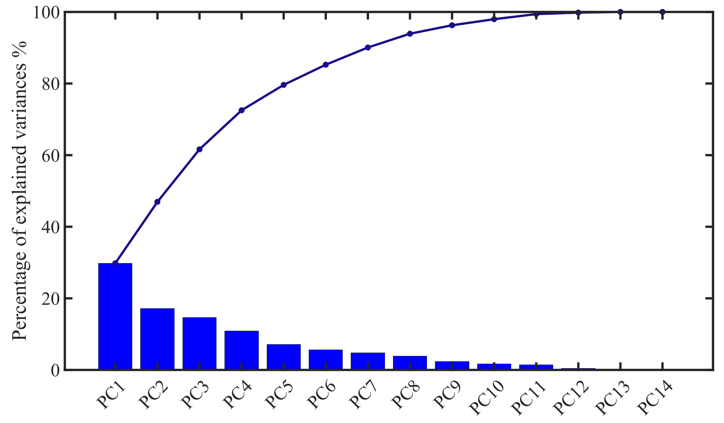
4.1. Principal Components Analysis Based on Mechanism and Knowledge

During the construction, mud formation is influenced by many factors such as soil type, mechanical parameters and rotation speed of the cutter, traverse speed of the dredger, dredge pump parameters, and so on. To monitor and control the dredging process, up to 255 specific real-time sensors were arranged to collect the operational data [27]. Figure 4 shows some of the related monitoring parameters and relationship in automatic control system.
As shown in Figure 4, some of the parameters are control variables, while some of them are only display variables that make the data visualization.
Soil property is an important factor affecting the construction process and efficiency of cutter suction dredgers. For different solidity and water-solubility, the mud concentration is limited by cutting performance and silt mixing. The cutter structure, pipeline diameter, and the motor power of pumps are all specific variables (constant), which were demonstrated according to the demand for rated productivity at the beginning of the design. However, the cutter speed, trolley trip, cutter ladder movement, and dredge pump rotation are all control variables that can be adjusted during the operation process in specific construction. When digging hard soil, the dredging depth should be reduced while enhancing the cutter speed to prevent the formation of large diameter mud balls and pipe blocking. When the dredging soil is sediment or silt, the pump velocity should be appropriately increased to reduce the mud concentration and avoid sedimentation or clogging in the pipeline.
According to the actual sensor system of cutter suction dredger “Chang Shi 10”, we firstly select 20 variables from the initial operational dataset as shown in Table 1.
Traditionally, the instantaneous productivity of the cutter suction dredger is the product of the flow and mud concentration.
P = C m · Q = C m · ( v · π r 2 )
where C m % represent the mud concentration; Q is the flow amount per hour; and v is the flow rate.
As shown in Table 1, we choose S21 (mud concentration) as the target variable. In actual dredging construction process, the change of flow rate in the sludge pipeline is one of the important factors affecting the flow. Thus, we delete the redundant variable S20 flow in the first step.
Meanwhile, the mud concentration is determined by the density of soil, water, and mud.
C m = γ m γ w γ s γ w
where γ m is the mud density; γ w is the water density; and γ s is the soil density.
Then we drop three redundant variables S223, S23, and S164 in the second step.
For the study period in this case, the ship works with just No.1 dredge pump. Thus, the variables related to No.2 dredge pump are non-meaningful to the productivity. Namely, S101 and S200 are dropped according to human analysis and finally we obtain the related variable set as:
X = S 8 , S 182 , S 108 , S 13 , S 9 , S 201 , S 12 , S 198 , S 100 , S 199 , S 165 , S 79 , S 80 , S 21
As described in Section 3.1, the selected variables X dataset based on human experience will be processed by PCA in this section. In addition, the contribution result is shown in Figure 5.
It is obvious that the top 10 principal components can represent more than 97% of the overall data. For the top two principal components, the dataset can be plot as Figure 6.
From the scatter plot of dataset in 2D figure, the correlation of the variables related to target S21 can be set as shown in Equation (28):
X = S 8 , S 182 , S 108 , S 13 , S 9 , S 201 , S 12 , S 198 , S 100 , S 199 , S 165 , S 79 , S 80
The most positively relevant variables to target can be further determined by the correlation matrix, as shown in Figure 7.
As the correlation matrix shows, the correlation between S21 and S199 is 0.48677, which means the discharge pressure of No.1 dredge pump affects the concentration most. It is consistent with the practical production. Pressure will influence the mud and water proportion that is pumped into pipeline. The variable S165 shows a correlation of 0.34628, which is also mentioned by other researchers [5,27]. The flow rate may determine the mud sedimentation during pipeline transportation. Furthermore, the vacuum correlation is 0.34152, since the vacuum gauge is installed on the upper part of the cutter, which is sensitive to the change of the mud concentration in the pipeline. Additionally, the angle of cutter ladder, the depth of dredging, and the trolley trip are all factors that affect the mud formation by operation controllers. However, for the discharge of the submersible pump, it is just the indirect factor to display the vacuum condition.
Meanwhile, it is indicated in the correlation matrix that there are five negative variables to the target. Thus, we obtain the final variables set most positively relevant to the target S21 as:
X * * = S 182 , S 108 , S 8 , S 9 , S 201 , S 198 , S 100 , S 199 , S 165
In general, the mud concentration is mainly inter-influenced by the dredge pump pressure, flow rate, vacuum, cutter ladder angle, dredging depth, and trolley trip.

4.2. Modeling Prediction Analysis

In this section, we choose the first segment series data and follow the steps given in Section 2.2 and Section 3.2 to train the proposed model. This segment series data is collected from the monitoring system with a frequency of 100 sample points per minute. We intercept a dataset of 18,000 for 3-hour working time zone and obtain final 16,764 data after the pre-process.

4.2.1. Learning Results Analysis

In terms of the variable’s selection process in Section 4.1, we use the most positively related nine parameters as input to predict the target output concentration C m % . Considering the data amount effects on the learning ability in data-driven models, we divide the input with a proportion of 6:4 and 7:3 to test the model twice. The learning results are shown in Figure 8 and Figure 9 respectively.
Concentration changes with the working conditions. As shown in the learning results, the normal range of the concentration is from 0 to 45%, which is a comprehensive result of the multiple factors interaction. High concentration is not necessarily good for the production since it may cause sedimentation or clogging in the pipeline. The results in this case are all normal and satisfactory. However, when it comes to the detailed comparison, the learning process with 60% of the dataset performs better than 70% dataset. For the 60% data training, its maximum and minimum error are 0.3091 and 0.0149 respectively. However, the maximum error is 0.526 in the 70% data training process. Also, as shown in Figure 10, for 60% dataset, the loss value decreases and then keeps steady in the training process. The error in testing falls and then keeps steady. However, for the 70% dataset, both training and testing error are less stable and consistent.

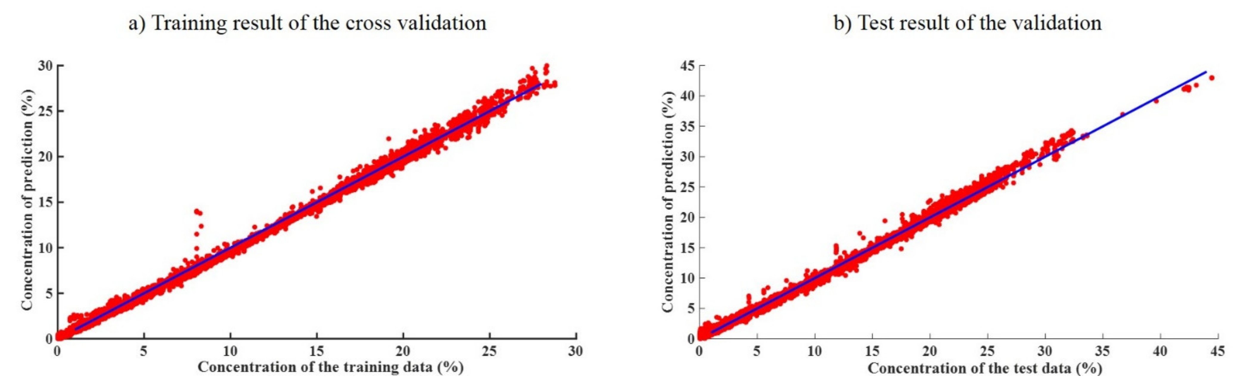
4.2.2. Cross Validation

Considering the necessary adaptability to dynamical changes, we use another dataset of 36,000 for 6-hour working time zone and obtain a final of 31,304 data samples for further cross validation to illustrate the proposed method’s effectiveness and generality. The learning results are shown in Figure 11.
It is obvious that the proposed method performs well in both training and testing processes. The average error in cross validation is 1.021%, which decreases since the data amount is becoming larger. In other words, data volume is essential for the deep learning method to function properly. This is just the advantage we explore in this novel model for prediction with operational “big data”. Especially, the model can be updated by upcoming new data for more accurate results.

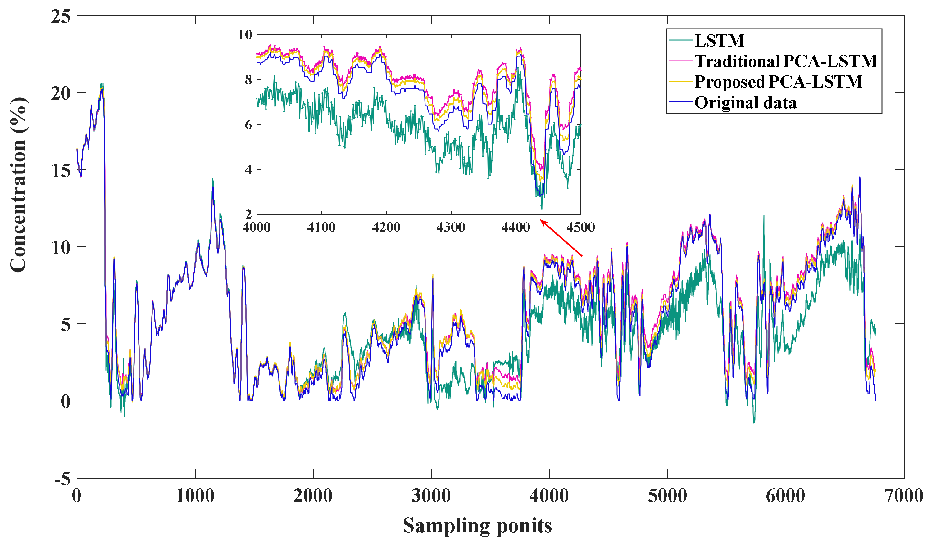
4.3. Comparative Study

This paper presents the novel PCA-LSTM method, which combines advantages of PCA and deep learning algorithm LSTM to manage big time-series data in operation monitoring systems. We compare the proposed method with other prediction methods including traditional PCA-LSTM and LSTM using the same dataset as Section 4.2 for further analysis. The results are shown in Figure 12 and Figure 13.
It is obvious in Figure 12 that the proposed method works better with a satisfactory error range. LSTM shows the maximum deviation because there is no variable selection before of the prediction process. Although it is a powerful tool to deal with the big series data for its special gate control function, it cannot give consideration to the variable analysis.
In Figure 13, it is easy to find that the novel PCA-LSTM performs better than both traditional PCA-LSTM and LSTM in the test. The yellow line in the figure marks the proposed PCA-LSTM, which has the lowest mean average error of 0.9213%. The green line marks the traditional PCA-LSTM, which shows a mean average error of 1.5301%. However, LSTM shows the worst result with a MAE (mean average error) of 2.0269%. The results differences are caused mainly because of the variable selection for the prediction model. As the input of the data-driven model, variable selection should be more focused with human knowledge and experience.
From a practical point of view, the comparative results are also analyzed by different evaluating indicators such as MAE (mean average error), R2 (coefficient of determination), and RMSE (root mean square error). As shown in Table 2, all of the models show a good performance with the coefficient of determination, which can explain the LSTM effectiveness. However, for the root mean square error, the proposed method takes on a better stability in the prediction result. The comparative results indicate that the control of input is essential to the machine learning methods.

5. Conclusions

This paper proposes the novel PCA-LSTM method for the productivity prediction of cutter suction dredger, wherein the deep learning process makes good use of the real-time operational monitoring data. The PCA method based on mechanism and knowledge is proposed to analyze the multiple parameters and select relevant variables from the operation process. Then the results are used as input into LSTM model to obtain the target prediction. This approach is also successfully validated by comparison against other methods on a real-world case in China. The productivity of cutter suction dredger is influenced by many correlated factors such as the soil characteristics, cutter parameters, mud pump performance, and pipeline layout. Thus, the mud concentration should be stabilized at a suitable value by comprehensive adjustment to improve its efficiency and productivity.
However, this is still a workable extension of deep learning application in the productivity prediction of cutter suction dredger. In the future, we will further construct the dynamical predictive models according to the changing working condition. When the operational parameters change dynamically under different conditions, the generated data should be classified into status space to study how the operation influences the dredging performance. Additionally, considering the sensors distance in the system, more factors on time-delay should be put up to improve the prediction accuracy.

Author Contributions

Conceptualization, K.Y.; methodology, K.Y.; software, K.Y.; validation, K.Y.; formal analysis, K.Y. and T.X.; data curation, K.Y., J.-L.Y. and B.W.; writing—original draft preparation, K.Y.; writing—review and editing, K.Y. and J.-L.Y.; visualization, K.Y.; supervision, S.-D.F.; funding acquisition, S.-D.F. All authors have read and agreed to the published version of the manuscript.

Funding

This research was funded by National Natural Science Foundation of China under Grant: 51679178 and 52071240.

Institutional Review Board Statement

Not applicable.

Informed Consent Statement

Not applicable.

Data Availability Statement

Not applicable.

Conflicts of Interest

The authors declare no conflict of interest.

References

  1. Kawakatsu, H.; Watada, S. Seismic evidence for deep-water transportation in the mantle. Science 2007, 316, 1468–1471. [Google Scholar] [CrossRef]
  2. Kuehl, S.; DeMaster, D.; Nittrouer, C. Nature of sediment accumulation on the Amazon continental shelf. Cont. Shelf Res. 1986, 6, 209–225. [Google Scholar] [CrossRef]
  3. Walsh, J.; Nittrouer, C. Contrasting styles of off-shelf sediment accumulation in New Guinea. Mar. Geol. 2003, 196, 105–125. [Google Scholar] [CrossRef]
  4. Tang, H.; Wang, Q.; Bi, Z. Expert system for operation optimization and control of cutter suction dredger. Expert Syst. Appl. 2008, 34, 2180–2192. [Google Scholar] [CrossRef]
  5. Wang, B.; Fan, S.; Jiang, P.; Xing, T.; Fang, Z.; Wen, Q. Research on predicting the productivity of cutter suction dredgers based on data mining with model stacked generalization. Ocean. Eng. 2020, 217, 108001. [Google Scholar] [CrossRef]
  6. Sierhuis, M.; Clancey, W.; Seah, C.; Trimble, J.; Sims, M. Modeling and simulation for mission operations work system design. J. Manag. Inf. Syst. 2003, 19, 85–128. [Google Scholar]
  7. Blazquez, C.; Adams, T.; Keillor, P. Optimization of mechanical dredging operations for sediment remediation. J. Waterw. Port Coast. Ocean. Eng.-ASCE 2001, 127, 229–307. [Google Scholar] [CrossRef]
  8. Lai, H.; Chang, K.; Lin, C. A Novel Method for Evaluating Dredging Productivity Using a Data Envelopment Analysis-Based Technique. Math. Probl. Eng. 2019, 2019, 5130835. [Google Scholar] [CrossRef]
  9. Pei, H.; Hu, C.; Si, X.; Zhang, J.; Pang, Z.; Zhang, P. Review of machine learning based remaining useful life prediction methods for equipment. J. Mech. Eng. 2019, 8, 1–13. [Google Scholar] [CrossRef] [Green Version]
  10. Wang, L.; Chen, X.; Wang, W. Research and analysis on construction output prediction of cutter suction dredger based on RBF neural network. China Harb. Eng. 2019, 39, 64–68. [Google Scholar]
  11. Guan, F.; Wang, W. Application of extreme learning machines in productivity prediction of trailing suction hopper dredger. Sci. Technol. Innov. 2020, 8, 58–61. [Google Scholar]
  12. Yang, J.; Ni, F.; Wei, C. Prediction of cutter suction dredger production based on double hidden layer BP neural network. Comput. Digit. Eng. 2016, 44, 1234–1237. [Google Scholar]
  13. Ren, L.; Sun, Y.; Cui, J.; Zhang, L. Bearing remaining useful life prediction based on deep autoencoder and deep neural networks. J. Manuf. Syst. 2018, 48, 71–77. [Google Scholar] [CrossRef]
  14. Wang, S.; Chen, Z.; Chen, S. Applicability of deep neural networks on production forecasting in bakken shale reservoirs. J. Pet. Sci. Eng. 2019, 179, 112–125. [Google Scholar] [CrossRef]
  15. Xu, W.; Peng, H.; Tian, X.; Peng, X. DBN based SD-ARX model for nonlinear time series prediction and analysis. Appl. Intell. 2020, 50, 4586–4601. [Google Scholar] [CrossRef]
  16. Hu, C.; Pei, H.; Si, X.; Du, D.; Wang, X. A prognostic model based on DBN and diffusion process for degrading bearing. IEEE Trans. Ind. Electron. 2019, 67, 8767–8777. [Google Scholar] [CrossRef]
  17. Deutsch, J.; He, D. Using deep learning-based approach to predict remaining useful life of rotating components. IEEE Trans. Syst. Man Cybern. Syst. 2017, 48, 11–20. [Google Scholar] [CrossRef]
  18. Zhang, C.; Lim, P.; Qin, A.K.; Tan, K.C. Multiobjective deep belief networks ensemble for remaining useful life estimation in prognostics. IEEE Trans. Neural Netw. Learn. Syst. 2016, 28, 2306–2318. [Google Scholar] [CrossRef] [PubMed]
  19. Wang, Y.; Zhang, Y.; Wu, Z.; Li, H.; Christofides, P. Operational Trend Prediction and Classification for Chemical Processes: A Novel Convolutional Neural Network Method Based on Symbolic Hierarchical Clustering. Chem. Eng. Sci. 2020, 225, 115796. [Google Scholar] [CrossRef]
  20. Chow, T.; Fang, Y. A recurrent neural-network-based real-time learning control strategy applying to nonlinear systems with unknown dynamics. IEEE Trans. Ind. Electron. 1998, 45, 151–161. [Google Scholar] [CrossRef]
  21. Malhi, A.; Yan, R.; Gao, R. Prognosis of defect propagation based on recurrent neural networks. IEEE Trans. Instrum. Meas. 2011, 60, 703–711. [Google Scholar] [CrossRef]
  22. Li, D.; Huang, D.; Yu, G.; Liu, Y. Learning Adaptive Semi-Supervised Multi-Output Soft-Sensors with Co-Training of Heterogeneous Models. IEEE Access 2020, 8, 46493–46504. [Google Scholar] [CrossRef]
  23. Yang, K.; Liu, Y.; Yao, Y.; Fan, S.; Ali, M. Operational time-series data modeling via LSTM network integrating principal component analysis based on human experience. J. Manuf. Syst. 2021, in press. [Google Scholar] [CrossRef]
  24. D’Agostino, R.B. Principal Components Analysis. In Handbook of Disease Burdens and Quality of Life Measures; Preedy, V.R., Watson, R.R., Eds.; Springer: New York, NY, USA, 2020. [Google Scholar] [CrossRef]
  25. Hochreiter, S.; Schmidhuber, J. Long short-term memory. Neural Comput. 1997, 9, 1735–1780. [Google Scholar] [CrossRef] [PubMed]
  26. Jafari, H.; Alipoor, A. A New Method for Calculating General Lagrange Multiplier in the Variational Iteration Method. Numer. Methods Partial. Differ. Equ. 2011, 27, 996–1001. [Google Scholar] [CrossRef]
  27. Bai, S.; Li, M.; Kong, R.; Han, S.; Li, H.; Qin, L. Data mining approach to construction productivity prediction for cutter suction dredgers. Autom. Constr. 2019, 105, 102833. [Google Scholar] [CrossRef]
Figure 1. The architecture of classical LSTM.
Applsci 11 08159 g001
Figure 2. The flowchart of proposed novel PCA-LSTM based on mechanism.
Applsci 11 08159 g002
Figure 3. The primary system highlighted in cutter suction dredger (1:150).
Applsci 11 08159 g003
Figure 4. The monitoring parameters related to dredging process and productivity.
Applsci 11 08159 g004
Figure 5. The percentage of explained variance for principal components.
Applsci 11 08159 g005
Figure 6. Scatter plot of the dataset after PCA.
Applsci 11 08159 g006
Figure 7. The correlation matrix of the variables.
Applsci 11 08159 g007
Figure 8. The learning results of 6:4 proportion.
Applsci 11 08159 g008
Figure 9. The learning results of 7:3 proportion.
Applsci 11 08159 g009
Figure 10. Loss curve of the different datasets.
Applsci 11 08159 g010
Figure 11. The learning result of cross validation.
Applsci 11 08159 g011
Figure 12. The training result of comparative study.
Applsci 11 08159 g012
Figure 13. The testing result of comparative study.
Applsci 11 08159 g013
Table 1. Initial variables from the operational dataset.
VariableDescriptionUnit
S8Angle of the cutter ladder
S9Depth of the dredgingm
S12Rotation speed of the submersible pumprpm
S13Rotation speed of the cutterrpm
S20Flowm3/h
S23Soil densitykg/m3
S79Distance of the swing movementm
S80Angle of the swing
S100Rotation speed of the No.1 dredge pumprpm
S101Rotation speed of the No.2 dredge pumprpm
S108Power of the cutter kw
S164Mud densitykg/m3
S165Flow ratem/s
S182Trolley tripm
S198Discharge pressure of the submersible pumpkPa
S199Discharge pressure of the No.1 dredge pumpkPa
S200Discharge pressure of the No.2 dredge pumpkPa
S201VacuumkPa
S223Water densitykg/m3
S21Mud concentration%
Table 2. Results analysis of the comparative study.
MAER2RMSE
Proposed PCA-LSTM0.04240.99990.0925
Traditional PCA-LSTM0.30630.98630.4054
LSTM0.33520.98280.5010
Publisher’s Note: MDPI stays neutral with regard to jurisdictional claims in published maps and institutional affiliations.

