Path Planning and Collision Avoidance in Unknown Environments for USVs Based on an Improved D* Lite

Abstract

Path planning and collision avoidance during autonomous navigation in unknown environments is a crucial issue for unmanned surface vehicles (USVs). This paper improves the traditional D* Lite algorithm and achieves multi-goal path planning and collision avoidance for USVs in unknown and complex environments. By expanding the adjacent search range and setting a safe distance for USVs, we solve the issue of limited steering maneuverability in USVs with fewer DOF during autonomous navigation. We propose an approach to optimize the planned path during navigation by comparing the estimated distance with the actual distance between the current waypoint and the goal waypoint. A minimum binary heap is used to optimize the priority queue of the D* Lite and significantly reduce the path search time. Simulation results show that the improved D * Lite can significantly reduce the path planning time, optimize the planned path and solve the issue of limited steering maneuverability in USVs. We apply the algorithm to a real USV for further tests. Experimental results show that the USV can plan an optimized path while avoiding both static and dynamic obstacles in complex environments with a safe distance during autonomous navigation.

1. Introduction

Due to the gradual deterioration in water quality [1], water quality monitoring is crucial for the protection of river systems. Unmanned surface vehicles (USVs) are widely used for water quality monitoring because of their advantages of low cost, high mobility and suitability for conducting dangerous tasks [2]. Path planning is a critical issue for autonomous navigation and collision avoidance in USVs. However, compared to other robots, such as UAVs, and due to the limited steering maneuverability and the fewer degrees of freedom (DOF) of USVs and the interference caused by wind and water flow, path planning is a more critical issue for autonomous navigation and collision avoidance in USVs.

Scholars have carried out much research on path planning [3,4,5]. The graph search algorithm of Dijkstra [6] is a classic path planning algorithm based on the breadth-first search strategy. However, the path search efficiency of the Dijkstra algorithm is very low due to its global path search strategy. The RRT* algorithm based on node sampling has been used to provide asymptotically optimal, computationally tractable and feasible paths in continuous radioactive space, and it gives a better navigation path than the Dijkstra algorithm [7]. However, the convergence rate of RRT* is slow. Hart and Nilsson proposed the A* algorithm [8]. It uses a heuristic function to estimate the path length from any node to the goal node. As a result, A* searches less space and is thus more efficient. It has been widely used in path planning and optimization [9]. However, it has to completely replan the path when the environment is changed, which makes it very inefficient in dynamic environments [10].

In 1994, Anthony Stentz, from the Robotics Institute of Carnegie Mellon University, proposed a Dynamic A* algorithm (D*) [11,12]. It has high path planning efficiency in partially known or continuously changing environments [13]. The D* was applied on the Mars probe launched by the U.S. and achieved huge success [14,15]. In 2004, Sven Koening introduced an approach involving incremental environmental information and proposed a Lifelong Planning A* algorithm (LPA*) [16], which significantly improves the path planning efficiency by reusing information [17]. The LPA* algorithm is efficient for path planning when it has specific start and goal nodes. However, it has to replan the whole path from the original start node to the goal node when a new obstacle appears on the path. To efficiently plan a path in a scenario with a changing start node and a fixed goal node, Koenig, S et al. developed a D* Lite algorithm based on the LPA* and D* algorithms [18,19]. It combines heuristic and incremental search and achieves fast path planning from a dynamic start node to a fixed goal node. D* Lite only takes into account the path information between the current node and the goal node while replanning. Therefore, its path planning efficiency is much higher than that of D* and LPA*. Thus, D* Lite is now widely applied to navigation systems for mobile robots and autonomous vehicles, including the prototypes of the Opportunity and Spirit Mars probes and the navigation system that won the Urban Challenge held by the Defence Advanced Research Projects Agency [20]. To further reduce the search space, improve the search efficiency and optimize the path in dynamic and complex environments, scholars are increasingly attempting to combine incremental search with sophisticated heuristic search for path planning. For example, in 2005, Dave Ferguson, et al. developed a delayed D* algorithm [21], which can improve the search efficiency by delaying the update of locally inconsistent nodes. KAl-Mutib et al. developed a D* Lite-based real-time multi-agent path planning algorithm for dynamic environments [22]. In 2015, Y. M. Sui, et al. proposed a D* lite label algorithm based on D* Lite, which can accelerate the path planning by preventing some nodes from being repeatedly updated. Yu, Jabin et al. improved the heuristic function of D* Lite to reduce the search area and accelerate the planning speed [23]. Yue, Weiya et al. proposed ID* Lite, which can increase the speed up to five times for a variety of benchmarks [24]. Yun, Soh Chin et al. proposed an enhanced D* lite and implemented it on a real-life situation using Team AmigoBot [25]. Le, An T. et al. identified the wasteful inconsistency-correction effort of D* Lite and proposed D* Lite with Reset for path planning in complex environments [26]. To find a route by which each vehicle can reach all depots to fulfil the demands of all the customers with the shortest travel distance, Barma, Partha Sarathi et al. developed a 2-opt guided discrete antlion optimization algorithm [27]. Comparison with heuristic approaches such as genetic algorithm and ant colony optimization showed that it has better performance.

This paper improves the traditional D* Lite algorithm in several ways and applies it to achieve multi-goal path planning and dynamic obstacle avoidance for USVs in unknown and complex environments. We expand the search neighbor and divide a sharp turn into several turning steps to solve the issue of limited steering maneuverability in USVs. To optimize the planned path, we compare the estimated distance with the straight distance from the current waypoint to the goal waypoint during autonomous navigation. A minimum binary heap is used to optimize the priority queue of the D* Lite, thereby reducing the path search time and improving the path search efficiency.

Section 2 introduces the concepts of D* Lite. We improve the D* Lite in Section 3 and analyse the simulation results in Section 4. In Section 5, we apply the improved D* Lite to a real USV for further tests. Finally, we conclude and discuss future research issues in Section 6.

2. D* Lite

2.1. Introduction of D* Lite

D* Lite searches reversely from the goal node to the start node. The key point of the algorithm is the assumption that all unknown areas are free space. Based on this assumption, it can incrementally plan the path. It finds a node from the adjacent nodes that is closest to the goal node by minimizing the distance ($rhs\left(s\right)$) between the current node and the goal node. When starting to move according to the path, it sets the current node as the start node. Thus, the path planning time is continuously reduced while moving towards the goal node.

We assume that $Succ\left(s\right)$ denotes the set of successor nodes of node s, $Pred\left(s\right)$ represents the set of predecessor nodes of node s, $c(s,s^{\prime })$ denotes the cost from node s to node $s^{\prime }$, $s_{start}$ is the start node, and $s_{goal}$ is the goal node. D* Lite represents the cost from a node to the goal node $s_{goal}$ with two estimated values, $g\left(s\right)$ and $rhs\left(s\right)$. The $g\left(s\right)$ denotes the estimated minimum cost from the goal node to the current node s. When expanding to the adjacent nodes of the current node s, the $rhs\left(s\right)$ of each adjacent node is recalculated to ensure that it is always the minimal estimated value. When $rhs\left(s\right)$ is calculated, it will be assigned to $g\left(s\right)$, as shown in Equation (1).

$$g\left(s\right)=rhs\left(s\right)$$

(1)

$rhs\left(s\right)$ is calculated by its successor’s estimated minimum cost of $g\left(s^{\prime }\right)$ and the cost of $c(s,s^{\prime })$ between node s and $s^{\prime }$, which is shown in the following equation:

$$rhs\left(s\right)=\left\{\begin{array}{cc}0\hfill & s=s_{goal}\hfill \\ mi{n}_{\mathrm{s}’}\subseteq \mathrm{Pred}\left(\mathrm{s}\right)(g\left(s^{\prime }\right)+c(s,s^{\prime }))\hfill & otherwise\hfill \end{array}\right.$$

(2)

where $g\left(s^{\prime }\right)$ is the minimal cost from the successor node $s^{\prime }$ to the goal node $s_{goal}$, and $c(s,s^{\prime })$ is the edge cost from node s to node $s^{\prime }$.

D* Lite stores searched nodes in a priority queue U and ranks these nodes according to their $key\left(s\right)$ value. The $key\left(s\right)$ contains two values of $k_1\left(s\right)$ and $k_2\left(s\right)$. The node with the smallest key value will be selected as the next node to be searched. The definitions of $k_1\left(s\right)$ and $k_2\left(s\right)$ are as follows:

$$k_1\left(s\right)=min(g\left(s\right),rhs\left(s\right))+h(s_{start},s)+k_m$$

(3)

$$k_2\left(s\right)=min(g\left(s\right),rhs\left(s\right))$$

(4)

where $k_m$ denotes the distance that the robot (USV in this paper) has moved. We use $k_m$ to avoid recalculating the priority queue when replanning the path, which can improve the computing efficiency.

We let $h(s_{start},s)$ be the estimated value from the current node s to the start node $s_{start}$, and we obtain the equation as follows:

$$h(s_{start},s)=\left\{\begin{array}{cc}0\hfill & s=s_{start}\hfill \\ c(s,s^{\prime })+h(s^{\prime },s_{start})\hfill & otherwise\hfill \end{array}\right.$$

(5)

During the process of path planning, D* Lite chooses an adjacent node of the current node s as the next node to expand, which has the smallest $key\left(s^{\prime }\right)$ value within all the adjacent nodes. The following equation shows the comparison of key values:

$$key\left(s\right)\le key\left(s^{\prime }\right)\Rightarrow \left\{\begin{array}{c}{k}_1\left(s\right)<k_1\left(s^{\prime }\right)\hfill \\ k_1\left(s\right)=k_1\left(s^{\prime }\right)\mathrm{and} k_2\left(s\right)\le k_2\left(s^{\prime }\right)\hfill \end{array}\right.$$

(6)

2.2. Disadvantages of D* Lite

As we know, D* Lite plans a path faster than other path planning algorithms such as A*, LPA* and D* in dynamic environments. However, there are some disadvantages that limit its application to USVs.

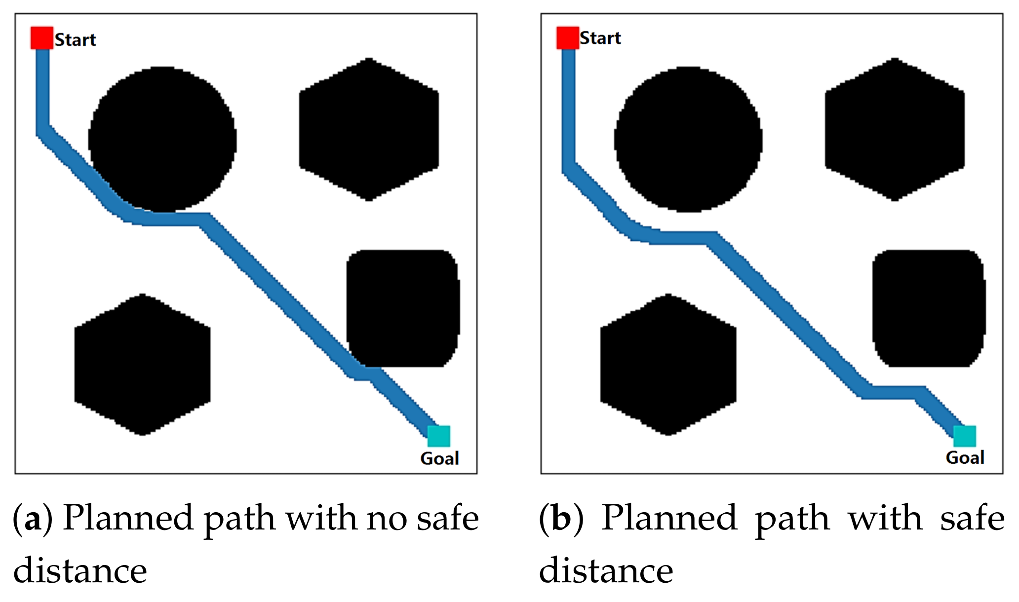
• The path planned by D* Lite is close to obstacles, which is unrealistic and risky for USVs.
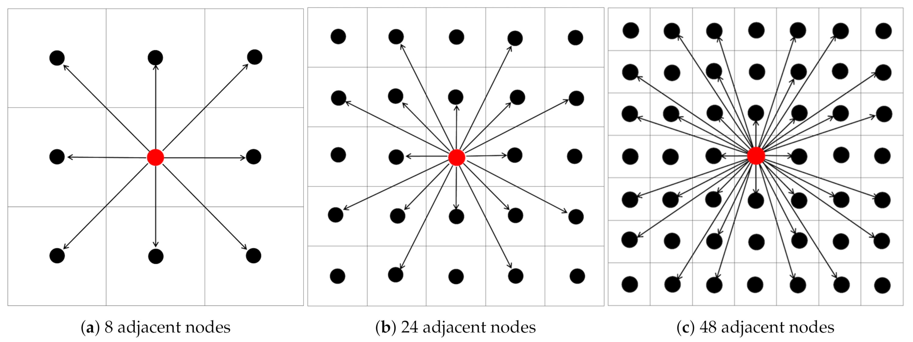
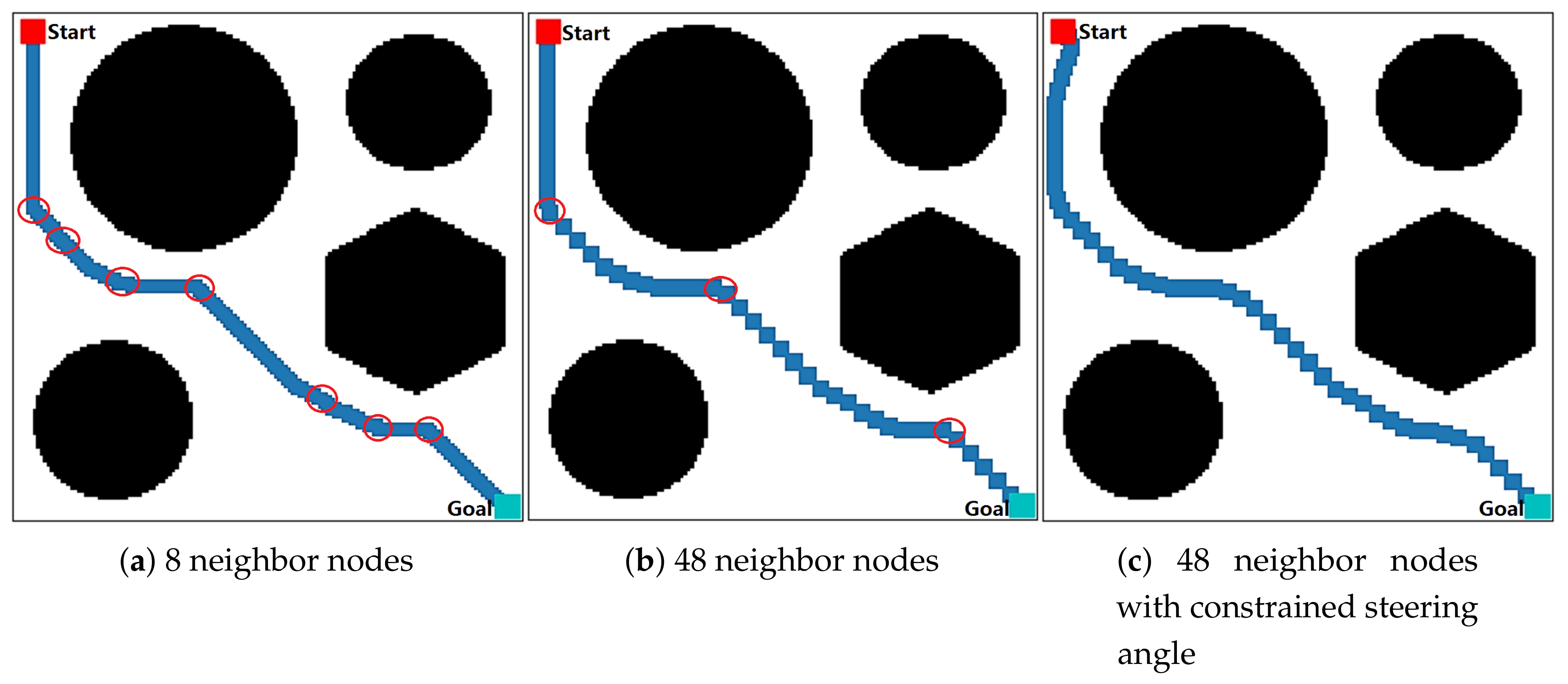
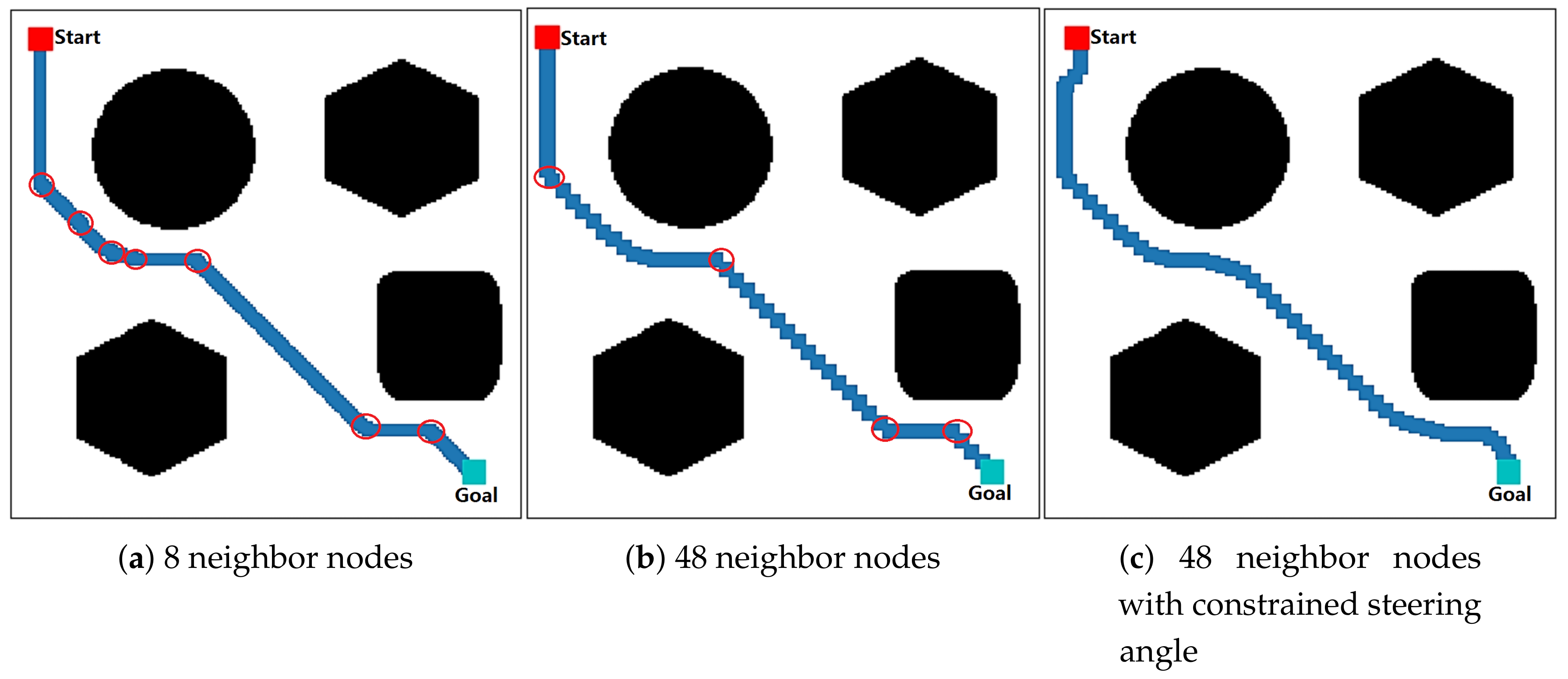
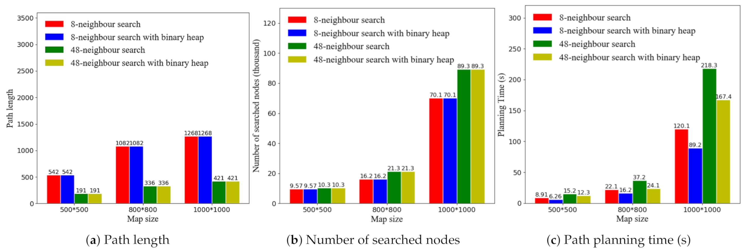
• D* Lite usually searches eight adjacent nodes for expansion. This means that the steering angle of USVs should be integral multiples of 45 degrees, which may be too much for a real USV to turn each time due to its limited steering maneuverability. We can increase the number of adjacent nodes to decrease the steering angle. However, this will significantly increase the search time for path planning. Thus, we should comprehensively consider the balance between the steering maneuverability of USVs and the path planning efficiency.
• D* Lite searches reversely from the goal node to the start node for path planning. This strategy is beneficial for replanning in dynamic environments. However, the planned path may have sharp turns [28], which increases the path length and results in a suboptimal path.
• D* Lite plans path between two nodes (the start and goal nodes). USVs may need to reach several specific positions during autonomous navigation. This means that it is necessary to achieve multi-goal path planning for USVs.
• D* Lite spends much computing time on the comparison of the key values of nodes in the priority queue U as well as push in and out operations on the priority queue. Each time, when we select a node from the priority queue U to expand, the key values of all nodes in the priority queue should be traversed and sorted, which is a time-consuming operation, and its time complexity is $O\left(n\right)$. When we plan a path within a large environment map with thousands of grids, the number of nodes in the priority queue for expanding is also increased, which can significantly decrease the search efficiency.

3. Improved D* Lite

To solve the disadvantages of D* Lite for USVs, we propose several approaches to improve the D* Lite. First, we set a safe distance between the path and obstacles to avoid collisions when a USV autonomously navigates along with the planned path. Second, we increase the number of adjacent nodes and add turning constraints to reduce the turning angle of the planned path. Third, we use a minimum binary heap to optimize the priority queue U to accelerate the planning process and improve the planning efficiency. Finally, we expand the D* Lite to be a multi-goal path planning algorithm.

3.1. Setting Safe Distance

As we know, the path planned by D* Lite is very close to obstacles, which increases the collision risk when a USV sails through these obstacles. To avoid obstacles, multi-criteria decision making (MCDM) can be used to identify risky areas around obstacles before path planning [29]. Another simple and widely used approach is to expand the size of obstacles to maintain a certain distance between the path and obstacles. Here, we also use an expansion approach to enlarge the boundary of obstacles in order to keep a safe distance between the USV and obstacles. The pseudocode in Algorithm 1 shows the main expansion procedure.

We let $map$ be the environmental map in Algorithm 1; $rows$ and $cols$ are the width and height of the map, and $distance$ represents a safe distance between the USV and obstacles. If node $map\left[i\right]\left[j\right]$ is an obstacle ($map\left[i\right]\left[j\right]=0$), all its surrounding nodes within the $distance$ will be set as “virtual” obstacles ($new\_map\left[x\right]\left[y\right]=0$). By this approach, we can expand the area of obstacles and set a safe distance between the planned path and obstacles.

Algorithm 1. Set safe distance.

Input: $map$, $rows$, $cols$, $distance$ Output: $new\_map$ 1: function SetSafeDis($map$, $rows$, $cols$, $distance$) 2:     set $new\_map=map$; 3:     for $i=0;i<rows;i++$ do 4:         for $j=0;j<rows;j++$ do 5:            if $map\left[i\right]\left[j\right]=0$ then   /* node $map\left[i\right]\left[j\right]$ is an obstacle */ 6:                for $x=i-distance;x<i+distance;x++$ do 7:                    for $y=j-distance;y<j+distance;y++$ do 8:                        if $0\le x<rowsand0\le y<cols$ then   /* node $x,y$ is in the map boundary */ 9:                           set $new\_map\left[x\right]\left[y\right]=0;$ /* set node $new\_map\left[x\right]\left[y\right]$ as an obstacle */ 10:                        else   /* out of the boundary */ 11:                           continue; 12:                        end if 13:                    end for 14:                end for 15:            end if 16:         end for 17:     end for 18:     return $(new\_map)$; 19: end function

3.2. Adjacent Node Expansion and Steering Angle Limitation

In practical applications, obstacle detecting sensors (e.g., Lidar, ultrasonic and stereo camera) can obtain detailed environmental information around the USV, which is much more substantial than the information on the eight adjacent nodes required by D* Lite. In addition, affected by limited steering maneuverability and inertia, USVs can only turn a limited angle each time. It is difficult to allow a USV to accurately turn an integral multiple of 45 degrees each time, which the original D* Lite constrains. To increase the flexibility of steering angles, we first expand the number of adjacent nodes from 8 to 24 and 48, respectively. Second, we add a restriction for the steering angle each time to simulate a more realistic scenario for USVs.

3.2.1. Adjacent Node Expansion

From Figure 1, we find that there are eight directions for the search if we plan a path based on eight adjacent nodes. When the number of adjacent nodes is expanded to 24 and 48, respectively, the search directions are also increased. This means that USVs may have more steering choices when planning a path. The relationship between the number of adjacent nodes, minimum steering angle and search directions is shown in

Table 1. Relationship between number of adjacent nodes, number of search directions and minimum steering angle.

Number of Adjacent Nodes	Number of Search Directions	Minimum Steering Angle
8	8	${45}^{\circ }$
24	16	$22.5^{\circ }$
48	32	$11.{25}^{\circ }$

.

We find from Table 1 that when we increase the number of adjacent nodes from 8 to 24, the search directions are increased from 8 to 16, and the minimum steering angle is significantly decreased from ${45}^{\circ }$ to $22.5^{\circ }$. This means that the search time is doubled while the minimum steering angle is reduced by two times. When the number of adjacent nodes is increased from 24 to 48, the minimum steering angle is decreased from 22.5 degrees to 11.25 degrees.

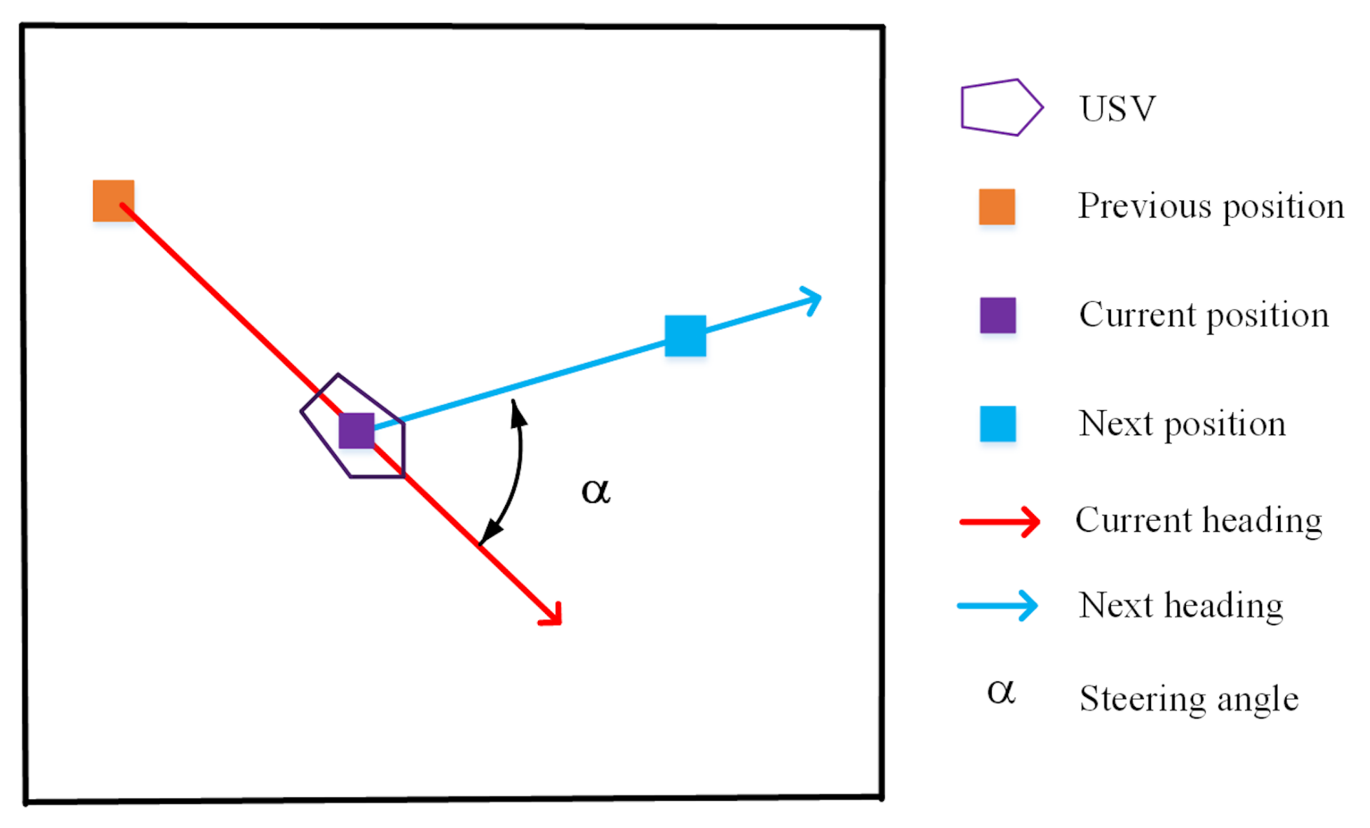
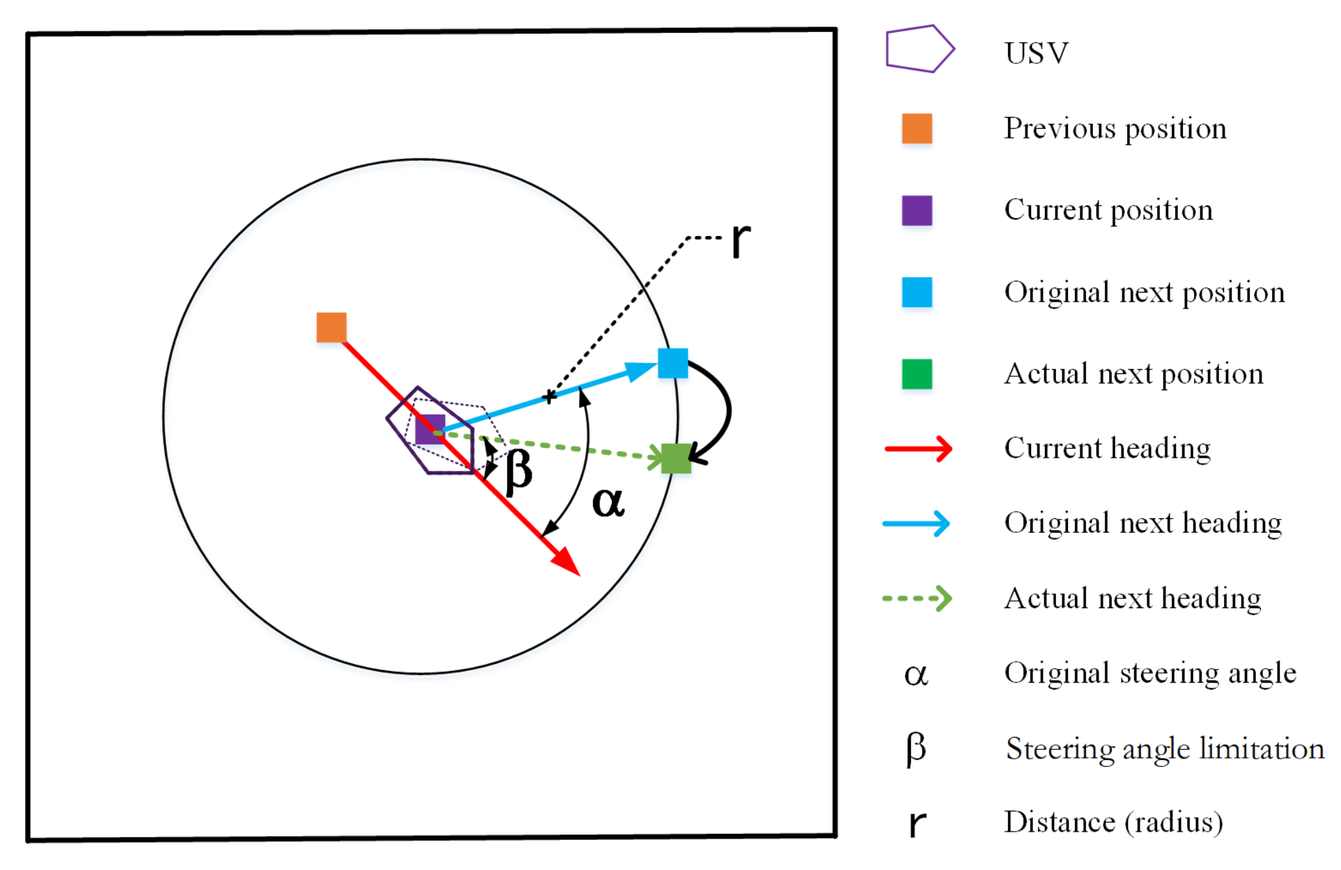
3.2.2. Steering Angle Limitation

Constrained by the steering maneuverability and the fewer DOF of USVs, the steering angle of USVs is limited. There may be still some sharp turns on the planned path even if we expand to 48 adjacent nodes for path planning. To plan a more realistic path for USVs, the algorithm should consider the steering angle limitation between two adjacent nodes along its path. When a turning angle is larger than the steering angle limitation that the USV can steer each time, we should divide it into several turning operations. Therefore, the steering angle can be constrained within the steering angle limitation. The definitions of USV heading and steering angle are as follows:

(1)

USV heading: the vector from the previous position to the current position of the USV. Initially, the USV heading is towards the goal position.

(2)

Steering angle: assume that the vector from the previous position to the current position is $\overrightarrow{A}$, and the vector from the current position to the next position is $\overrightarrow{B}$. We define the steering angle as the angle between $\overrightarrow{A}$ and $\overrightarrow{B}$, which is shown in Figure 2.

When the steering angle ($\alpha$) is larger than the steering angle limitation of the USV ($\beta$), we should divide the turning operation into several steps, and we only turn an angle no more than the steering angle limitation in each step. We let the distance between the current position and the next position be the radius R. Because $\alpha >\beta$, we turn the USV to the next position with a limited steering angle $\beta$. Thus, we can obtain a new position as the next position for path planning. Figure 3 demonstrates the turning procedure between two original positions and the calculation for the new next position.

Assume that the coordinate of the current position is ($x_1$, $y_1$). The USV firstly calculates the current heading according to the previous and current positions. Afterwards, the original next position ($x_2$, $y_2$) and original steering angle $\alpha$ are calculated. If the original steering angle is larger than the USV’s maximum steering angle ($\alpha >\beta$), then we calculate the actual next position (x, y) according to Equation (7). The process is repeated until the USV’s heading is turned towards the original next position.

$$\left\{\begin{array}{c}x=(x_1-x_2)\times cos(\alpha -\beta )-(y_1-y_2)\times sin(\alpha -\beta )+x_2\hfill \\ y=(y_1-y_2)\times sin(\alpha -\beta )+(x_1-x_2)\times cos(\alpha -\beta )+y_2\hfill \end{array}\right.$$

(7)

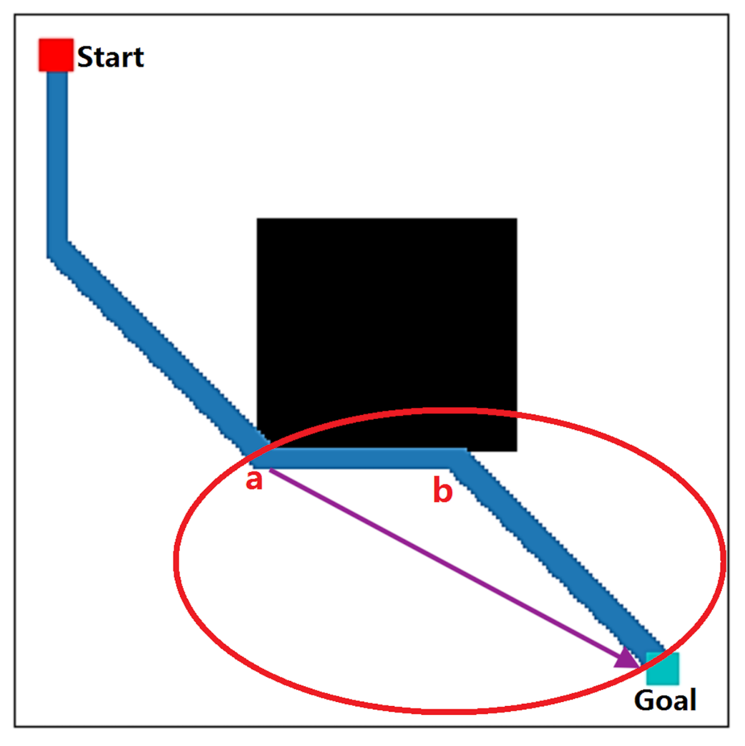
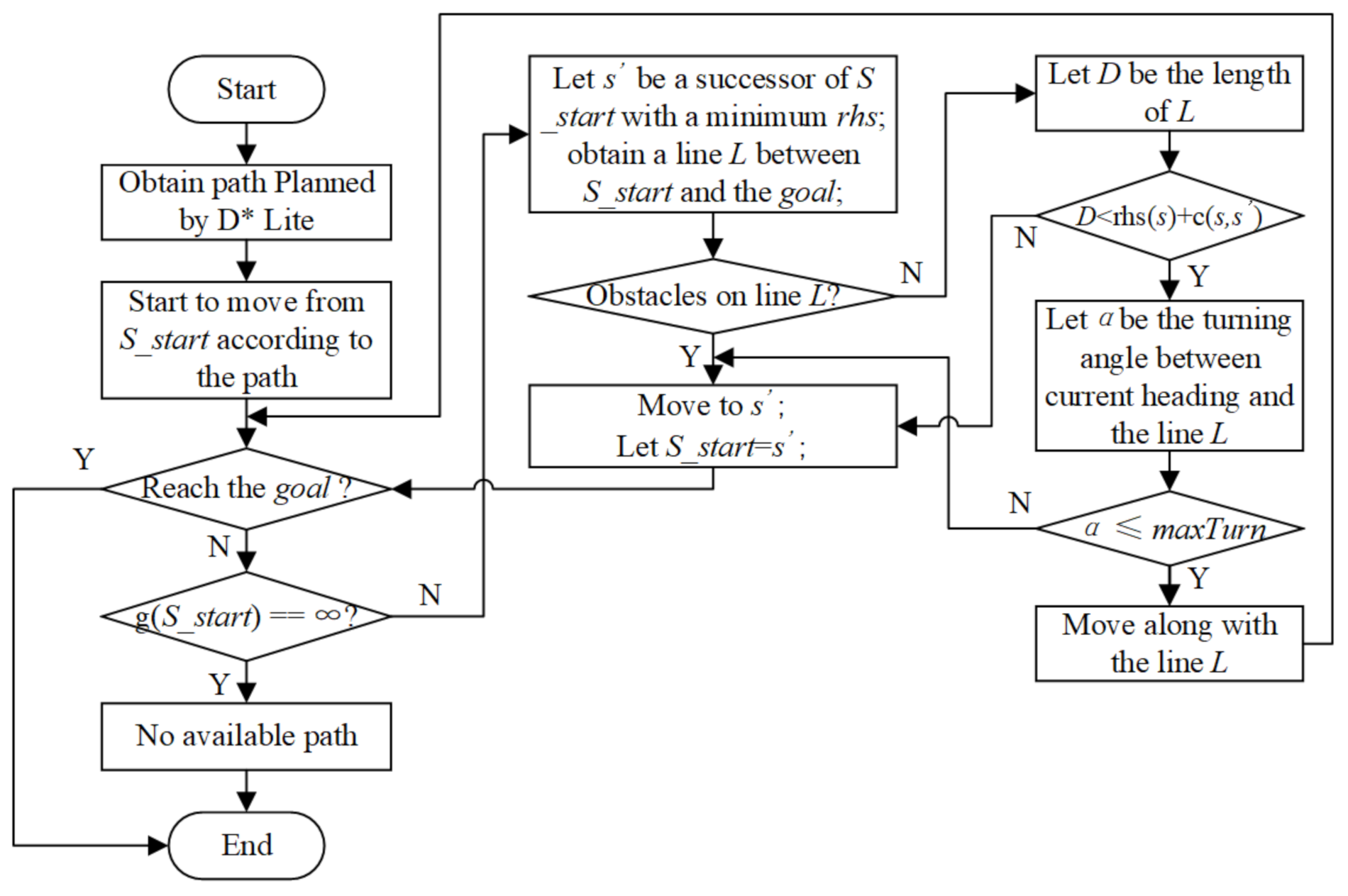
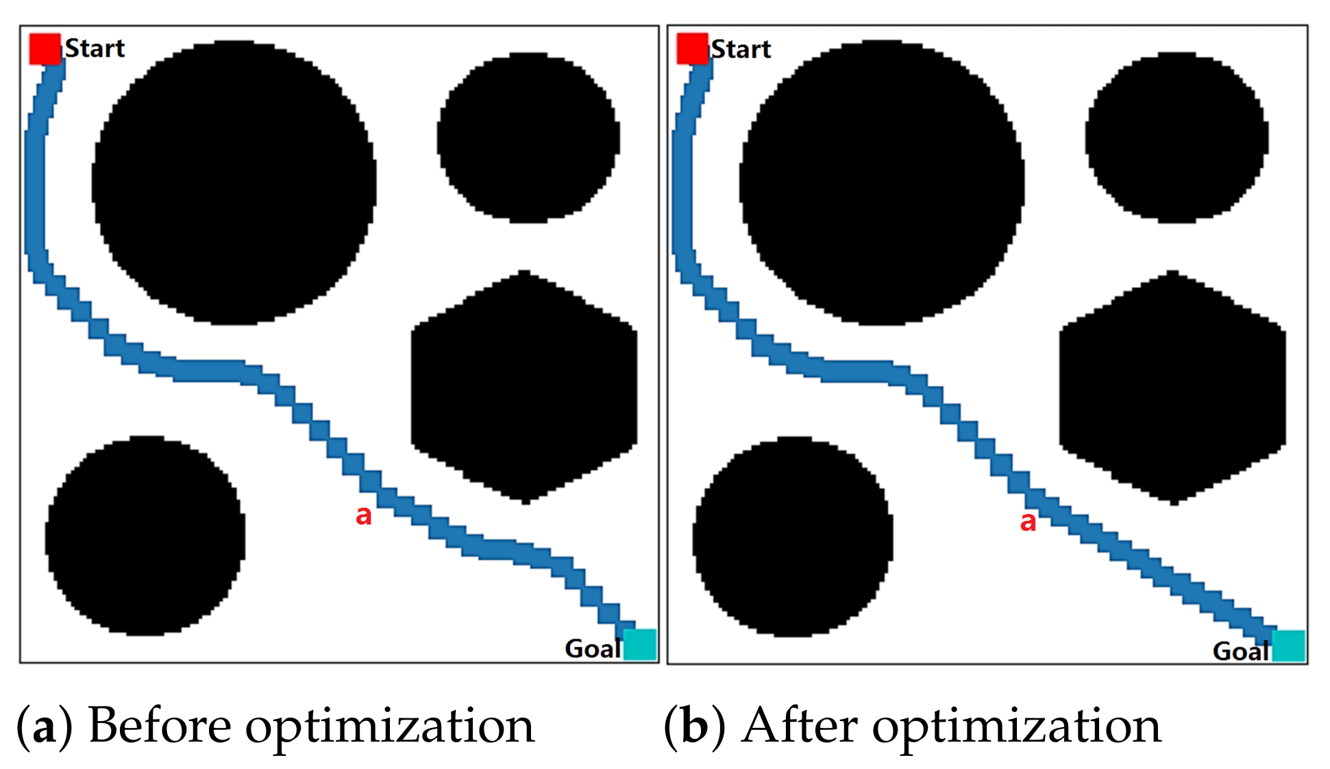
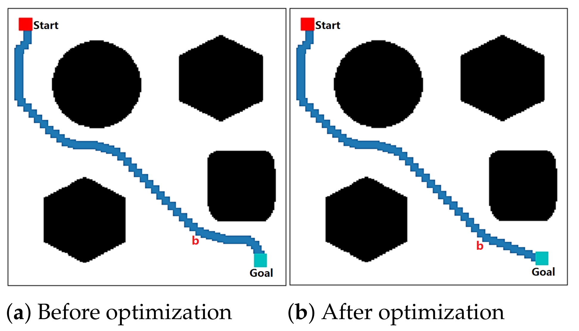
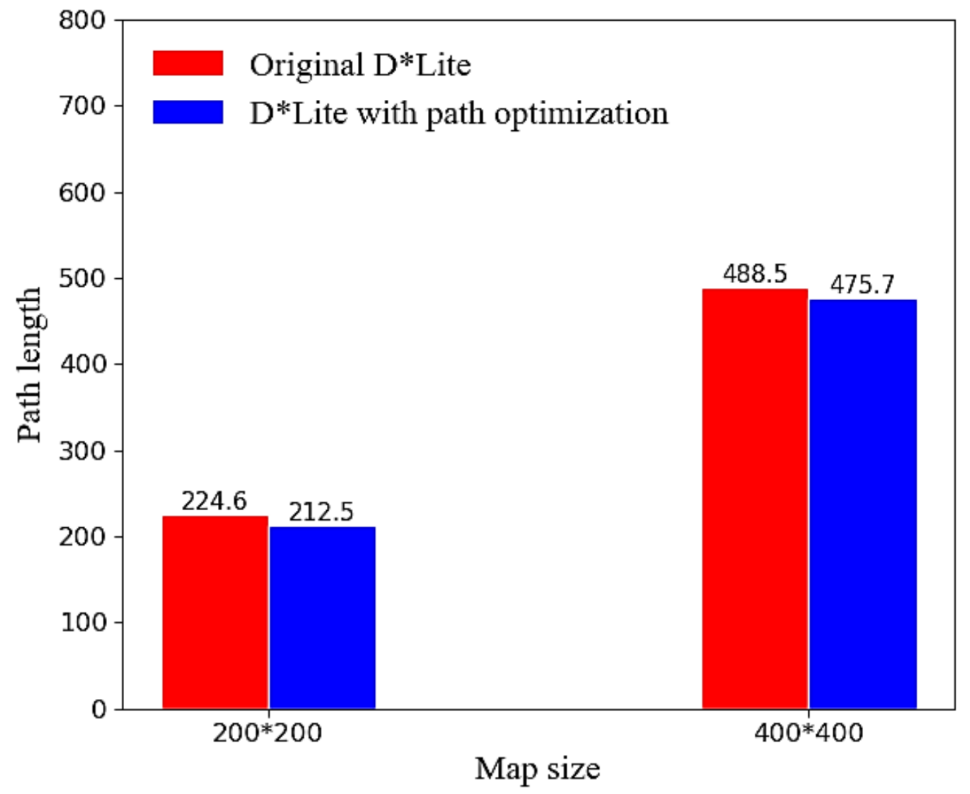
3.3. Path Optimization

The reversed path planning in D* Lite is beneficial to replanning when there are dynamic obstacles. However, there may also be some redundant turns in the path, which increases the path length. Figure 4 shows a simple path planned by the D* Lite. We find that when D* Lite starts to plan a path from the goal node to the start node, it detects an obstacle at position b and makes a left turn towards position a to avoid the obstacle. Finally, it finds a path from the goal node to the start node. However, we find that the path between position a and the goal node is not optimal. It contains an unnecessary turn towards position b. We can reduce the path if we can let the USV drive straight from position a to the goal node.

To optimize the path, we set the line from the current node s to the goal node as l. We compare the $rhs\left(s\right)$ value with the length of l. If there is no obstacle along the line l and the $rhs\left(s\right)$ value is smaller than the length of l, then we replace the original path segment with the straight line. Figure 5 shows the main procedure of path planning and optimization.

The main steps of the planning and optimization precedure are as follows:

1.

Plan the path using D* Lite.

2.

Start to move from the start node $S_{start}$ to the goal node $S_{goal}$.

3.

Set the current node as s and calculate the $rhs$ value of its all the successor nodes. Let node $s^{\prime }$ represent the node with the smallest $rhs$ value of the successor nodes.

4.

Set a line L from node s to the goal node $S_{goal}$.

5.

If there is no obstacle along line L,

(a)

Let D be the length of L.

(b)

If $D\ge rhs\left(s^{\prime }\right)+c(s,s^{\prime })$, move to node $s^{\prime }$; go to step (3).

(c)

Otherwise, if $\alpha >maxTurn$, move to node $s^{\prime }$; go to step (3). Otherwise, move from node s to the goal node $S_{goal}$ directly.

6.

Otherwise, if there is an obstacle along line L,

(a)

Move to node $s^{\prime }$.

(b)

Go to step (3).

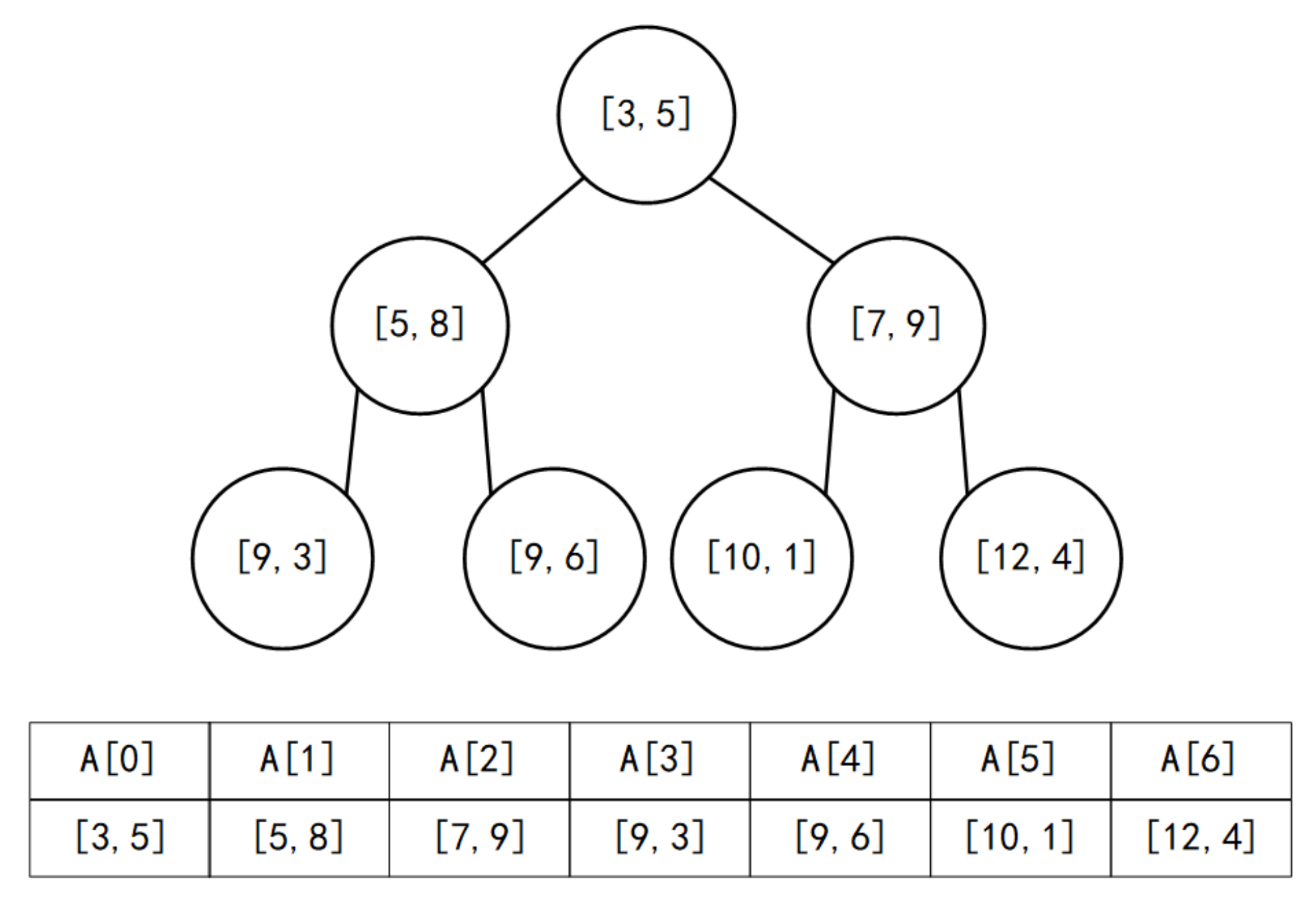
3.4. Optimization of Priority Queue

The original D* Lite does not rank nodes in the priority queue U. Thus, it has a time complexity of $O\left(1\right)$ when it pushes a new node into the queue for further expansion. However, the time complexity is significantly increased to $O\left(n\right)$ when it pops up a node with the smallest key from the priority queue to expand each time, which is a time-consuming operation for path planning. Therefore, the time complexity for path expansion is $O\left(n^2\right)$ if there are n nodes in the priority queue, which is a relatively low efficiency for a complex environment with thousands of nodes.

To improve the path search efficiency and decrease the search time, we use the minimum binary heap [30,31] to optimize the priority queue. Figure 6 shows an example of using the minimum binary heap to store data. The node with the smallest key value is on the top of the heap and is stored on the first position of the linear array. All its predecessor nodes have larger key values and are stored on the second and third positions of the array, respectively.

D* Lite has three types of operations on the priority queue: (1) pop up the node with the smallest key value; (2) search a specific node in the priority queue; (3) push a node into the priority queue. The characteristics of binary heap guarantee the stability of nodes in the priority.

Table 2. Time complexity for conventional priority queue and minimum binary heap.

Operation	Time Complexity
	Conventional Queue	Minimum Binary Heap
Pop up	$O\left(n\right)$	$O\left(1\right)$
Push in	$O\left(1\right)$	$O\left(lo{g}_n\right)$
Search	$O\left(n\right)$	$O\left(lo{g}_n\right)$

is a comparison of the time complexity of the conventional priority queue and the minimum binary heap. We find that the time complexity of the pop up operation on the conventional priority queue is $O\left(n\right)$. When we replace the conventional priority queue with the minimum binary heap, the time complexity of the pop up operation is sharply decreased to $O\left(1\right)$. We find a similar result on the search operation. However, the time complexity for the push operation of the minimum binary heap is larger than that of the conventional queue. On the whole, the time complexity of the minimum binary heap is much lower than that of the conventional priority queue.

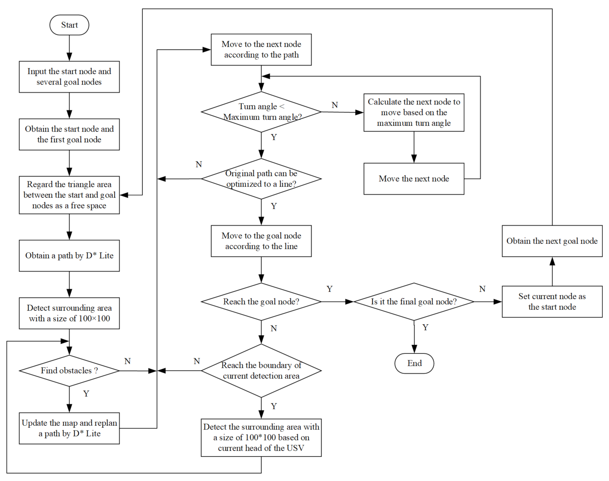
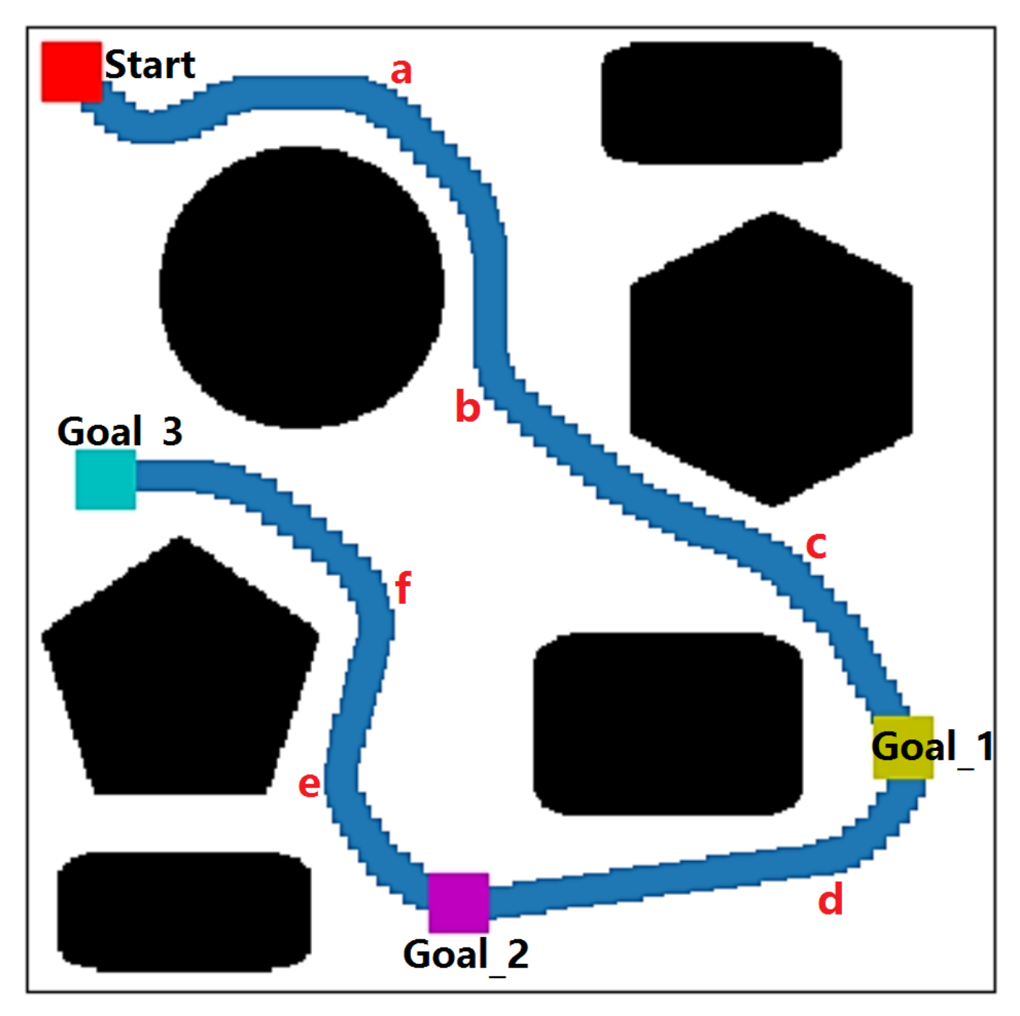
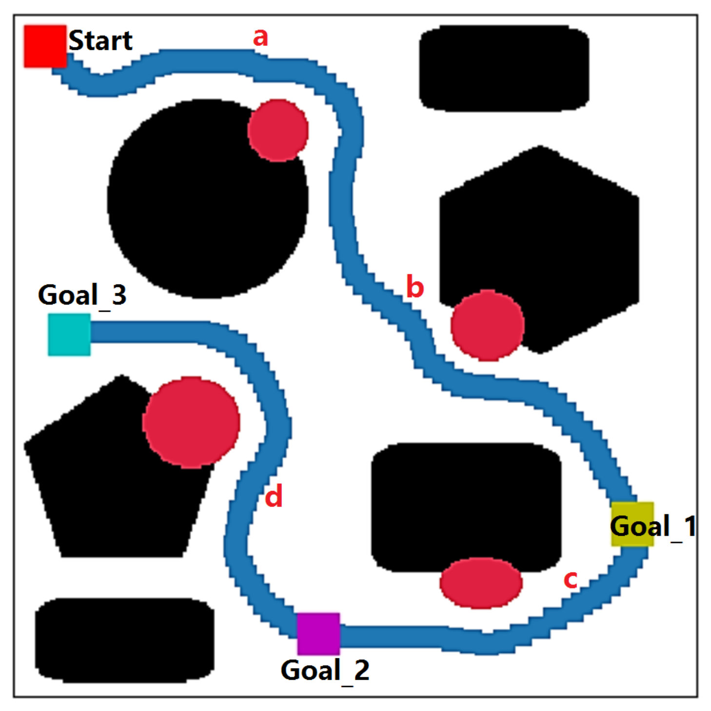
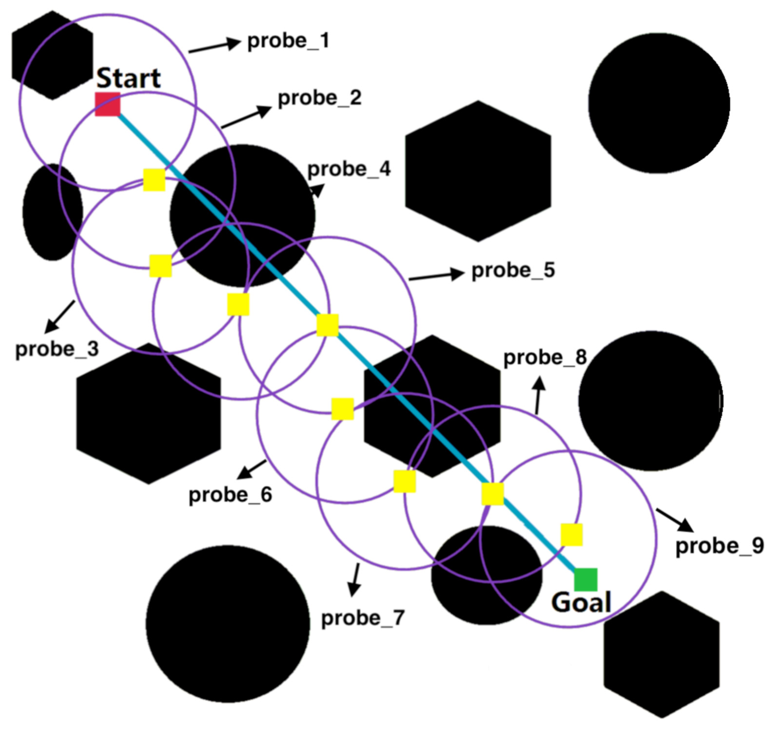
3.5. Multi-Goal Path Planning in Unknown Environment

In practical applications, sensors on the USV can continuously sense the local surrounding environment during autonomous navigation. Thus, it can only plan a local path based on the local environment information obtained by sensors each time. Furthermore, USVs may need to arrive at several special positions for water quality monitoring or water sampling. Therefore, there are several goal nodes along the planned path. Thus, the D* Lite must be expanded to support multi-goal path planning. Figure 7 shows the main procedure of multi-goal path planning in unknown environments.

The main steps of multi-goal path planning in unknown environments are as follows:

1.

Initialize the start and goal nodes. Assume that the whole region from the start node to the goal node is a free space (i.e., no obstacles). Then, plan a path from the goal node to the start node with D* Lite.

2.

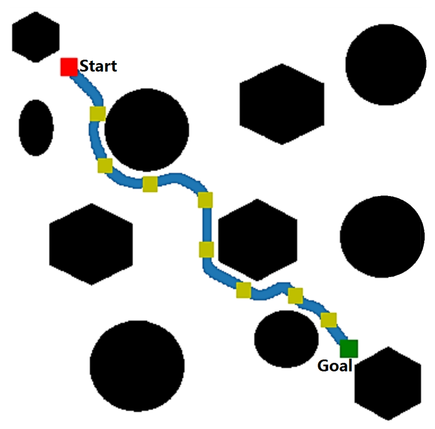
The USV detects environmental information with its sensors, starting from the current node, and verifies whether the goal node is within the detected area. If so, the USV proceeds to the goal node according to the path planned with D* Lite and the path planning procedure is finished. Otherwise, go to step (3).

3.

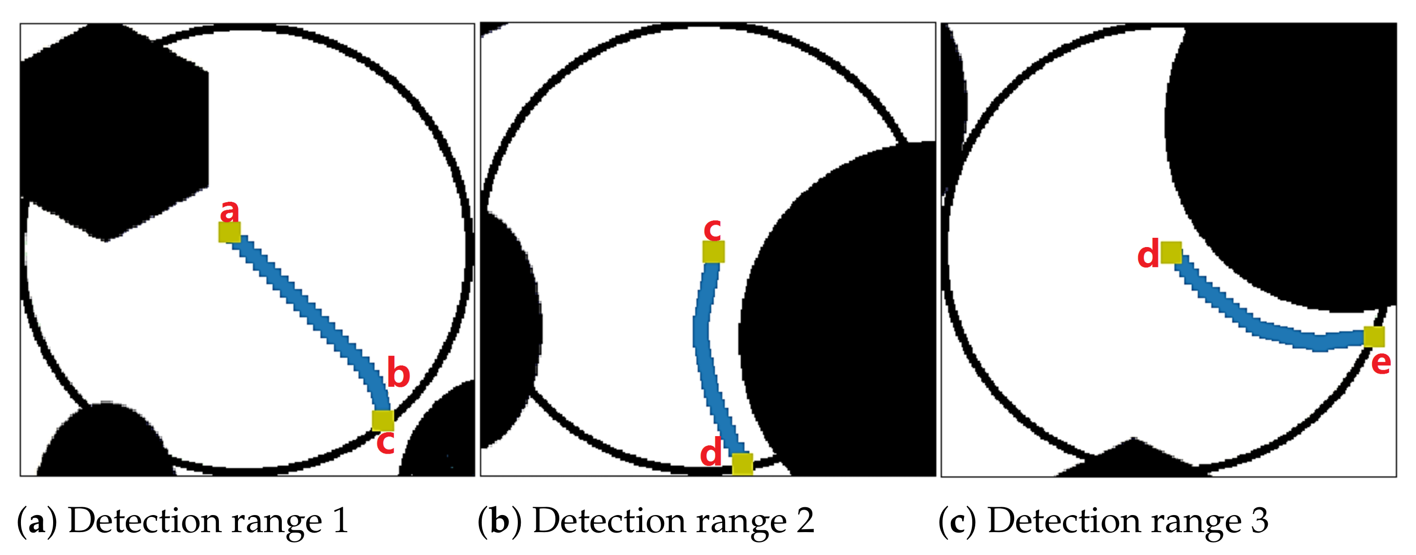
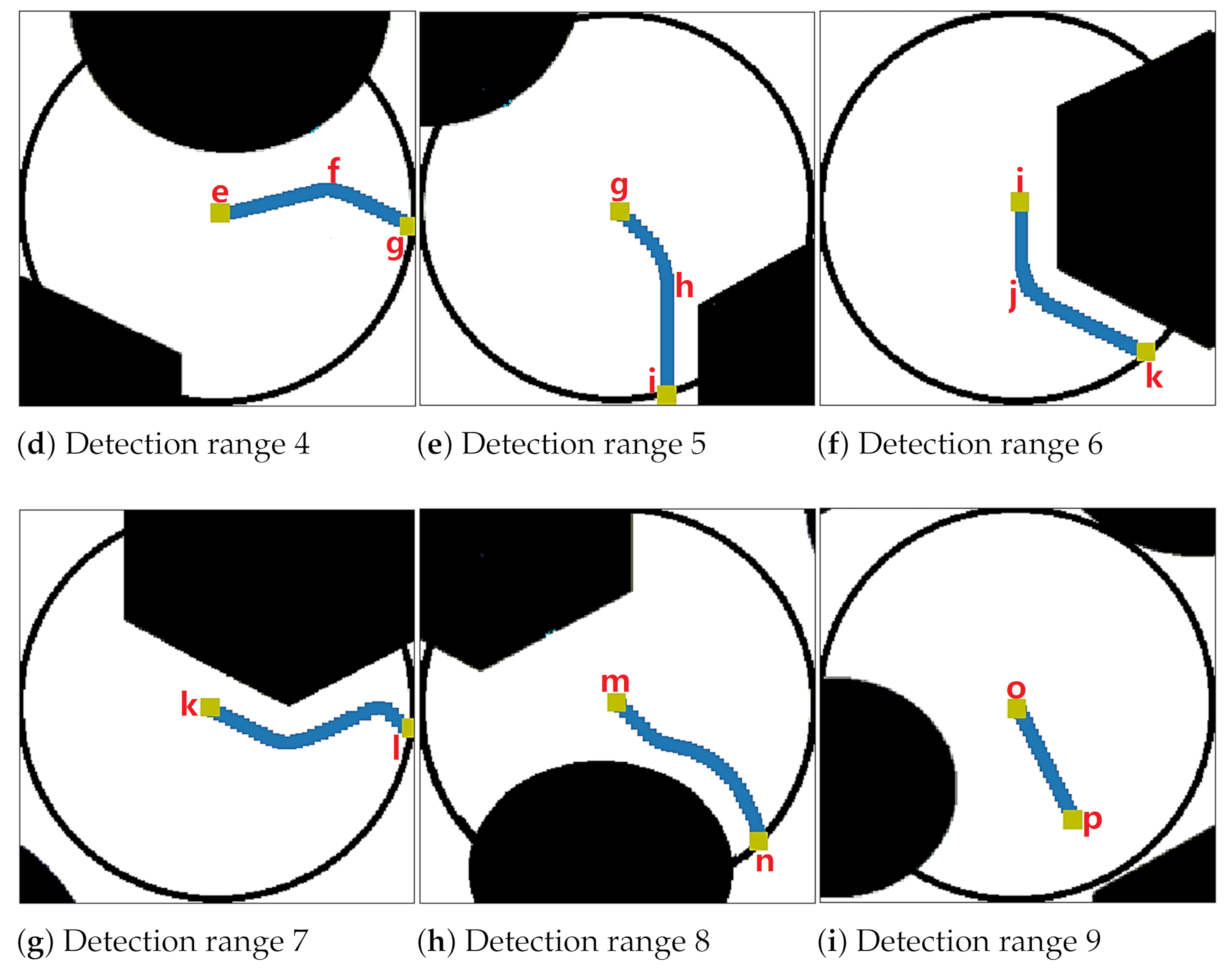
Use D* Lite to plan routes within the detected area. When changes to the environmental information within the detection range are detected, start dynamic route planning until travelling to the boundary of the detected area. Then, the local path planned within the detected area is finished. Set the current node as the start node and plan a new local path within the detected area, and go to step (2).

4. Simulation Results and Analysis

4.1. Path Planning with Safe Distance

We define an experimental environment on a map with 400 × 400 pixels. The black shapes are obstacles, and the white regions are free space. We set the start node at the upper left of the map and the goal node at the lower right of the map. In addition, we set the safe distance as 10 pixels. We assume that the USV only moves one pixel each time. Figure 8a shows the path planned by the original D* Lite. We find that the planned path is very close to the obstacles. Figure 8b shows a path planned with a safe distance based on Algorithm 1. It shows that there is at least a 10-pixel distance between obstacles and the path. Thus, we improve the safety for the USV to sail through obstacles.

4.2. Path Planning with Constrained Steering Angle

In practice, USVs can only turn a limited angle each time. We assume that a USV’s maximum steering angle each time is 30 degrees, and the safe distance is 10 pixels. We define two experimental maps with a size of 200 × 200 and 400 × 400 pixels, respectively. We perform the simulations with 8 neighbor nodes, 48 neighbor nodes and 48 neighbor nodes with a constrained steering angle, respectively. Figure 9 and Figure 10 show the experimental results on the two maps, respectively.

From Figure 9a and Figure 10a, we find that because the steering angle of eight-neighbor search is always an integral multiple of 45 degrees, many turns (marked with red circle) have a steering angle larger than the maximum steering angle of the USV. Therefore, we argue that the search approach with eight neighbor nodes is unsuitable for a real USV.

We increase the number of neighbor nodes to 48 and obtain the planned path shown in Figure 9b and Figure 10b. We find that the number of turns exceeding the maximum steering angle is reduced. This is because the steering angle of the 48-neighbor search is always an integral multiple of 11.25 degrees. In most cases, the turning degree of the planned path is no more than 30 degrees. However, the planned path still has three turns exceeding the maximum steering angle near obstacles.

We add a constrained steering angle to the algorithm with 48-neighbor search and obtain new paths, as shown in Figure 9c and Figure 10c. Compared to the planned paths without the constrained steering angle, the new paths are much smoother, and all the steering angles are smaller than the maximum steering angle of the USV.

Table 3. Number of exceeding steering angles.

Map Size	200 × 200			400 × 400
Search approach	8-neighbor	48-neighbor	48-neighbor with constrained steering angle	8-neighbor	48-neighbor	48-neighbor with constrained steering angle
Number of searched nodes	745	1813	1869	896	2516	2521
Planning time (s)	1.16	4.07	4.14	2.07	5.47	5.63
Number of sharp turns	25	5	0	29	7	0

shows the experimental results of the number of searched nodes, path planning time and the number of sharp turns exceeding the maximum steering angle based on different neighbor search approaches and the constrained steering angle.

We find that when the number of neighbor nodes is increased from 8 to 48 on the 200 × 200 map, the number of searched nodes is also increased from 745 to 1813. This is because when we increase the number of neighbor nodes, there are more nodes to be expanded during the path planning process. Thus, the planning time is also increased from 1.16 s to 4.07 s. However, the number of sharp turns exceeding the maximum steering angle is significantly decreased from 25 to 5 when the number of neighbor nodes is increased from 8 to 48. When we add the constrained steering angle, the number of searched nodes and the planning time are slightly increased, but the number of sharp turns is significantly decreased to 0. We find similar results on the 400 × 400 map. Thus, we can conclude that the constrained steering angle can ensure that the planned path is more realistic and can be applied to USVs in practice.

4.3. Path Optimization

We apply the path optimization approach proposed in Section 3.3 on the 200 × 200 and 400 × 400 maps, respectively. Figure 11 and Figure 12 show the planned paths.

Figure 11a shows that there are several turns on the planned path between position a and the goal node. However, optimized by the algorithm, the path between position a and the goal node is a straight line in Figure 11b. This is because when the USV arrives at position a, it finds that there is no obstacles on the straight line between position a and the goal node, and the distance of the straight line is shorter than the planned path. Therefore, the USV will move directly along the straight line to the goal node. We obtain a similar result on the 400 × 400 map (Figure 12). Figure 13 shows that the length of the optimized path on the 200 × 200 map is decreased from 224.6 to 212.5 (5.4% reduction). The path length is also decreased from 488.5 to 475.7 (2.6% reduction) on the 400 × 400 map.

Based on the observation above, we conclude that the path optimization algorithm can further optimize the path with a shorter length while almost not deteriorating the planning time.

4.4. Optimization of Priority Queue

In this section, we use the minimum binary heap to improve the priority queue of D* Lite. To evaluate the efficiency of the minimum binary heap, we simulate D* Lite with 8-neighbor node search, 8-neighbor node search with the minimum binary heap, 48-neighbor node search and 48-neighbor node search with the minimum binary heap. We compare their path length, the number of searched nodes and path planning time on three maps of 500 × 500, 800 × 800 and 1000 × 1000, respectively. Experimental results are shown in Figure 14.

From Figure 14a, we find that when we apply the minimum binary heap to the 8-neighbor and 48-neighbor searches, respectively, on the three maps, their path lengths are the same as in the original neighbor search approaches separately. This is because the minimum binary heap only improves the storage structure of the priority queue, but the search strategy is the same, resulting in the same path length and number of searched nodes. We also find that the path length of 48-neighbor node search is much smaller than that of the eight-neighbor node search. We believe that this is because that the 48-neighbor node search has more choices to select a steering angle for turning, which can lead to a shorter planned path. We also find that when we increase the map size from 500 × 500 to 800 × 800 and 1000 × 1000, respectively, the path length is also increased.

Figure 14b shows that the number of searched nodes is also not changed when we use the minimum binary heap or not in D* Lite. However, when we increase the number of neighbor nodes for the search, more neighbor nodes will be expanded, resulting in an increase in the number of searched nodes. Similar to the path length, the number of searched nodes is also increased accordingly when the map size is increased.

Figure 14c shows that on the same map, the path planning time of the 48-neighbor node search is a little bit longer than that of the eight-neighbor node search. The path planning time is increased from 8.91 s to 15.2 s, from 22.1 s to 37.2 s and from 120.1 s to 218.3 s, respectively, on the three maps with different map sizes. We believe that this is because the 48-neighbor node search needs to search more neighbor nodes, which increases the path planning time. When we apply the minimum binary heap to the eight-neighbor node search on the 500 × 500 map, the path planning time is decreased from 8.91 s to 6.26 s (29.7% reduction). We find similar results on the 800 × 800 and the 1000 × 1000 maps.

Based on the analysis above, we conclude that the minimum binary heap can significantly decrease the path planning time for D* Lite while still obtaining the same optimized path.

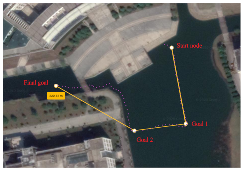
4.5. Simulation of Multi-Goal Path Planning

4.5.1. Multi-Goal Path Planning in Static Environment

In this section, we improve the D* Lite to support multi-goal path planning and apply it to a static environment. We set one start node and three goal nodes in the static environment. Figure 15 shows the static environment and the planned path.

First, the improved D* Lite plans a path from the goal node ($Goal\_1$) to the start node. Affected by the obstacles and safe distance, the algorithm plans a straight line between $Goal\_1$ and position c, and then turns left to position b. Influenced by the two obstacles above, there is a curve between positions b and c. Constrained by the maximum steering angle, the path slightly turns left and moves towards the start node. After planning, the USV starts to move from the start node to node $Goal\_1$ along the planned path. When the USV reaches $Goal\_1$, the algorithm starts to plan a new path from $Goal\_2$ to $Goal\_1$. Finally, the USV reaches the destination of $Goal\_3$ according to the planned path.

4.5.2. Multi-Goal Path Planning in Dynamic Environment

To simulate the path planning in a dynamic environment, we set four random dynamic obstacles (red ellipses) based on the same environment in Figure 15. The simulation result is shown in Figure 16.

First, the improved D* Lite plans the same path shown in Figure 15, and the USV starts to move from the start node to $Goal\_1$. When it reaches position a, a dynamic obstacle emerges, and the algorithm replans a new path from $Goal\_1$ to position a to avoid the obstacle and keep a safe distance between the USV and the obstacle. When the USV arrives at position b, another obstacle emerges and the algorithm has to replan a new path from $Goal\_1$ to position b. When the USV reaches $Goal\_1$, the algorithm starts to plan a path from $Goal\_2$ and $Goal\_1$. A third obstacle emerges when the USV arrives at position c. The algorithm replans a new path between goal node $Goal\_2$ and position c. Finally, the USV reaches $Goal\_2$ and stops at the destination of $Goal\_3$.

4.6. Path Planning in Unknown Environments

Nowadays, Lidar, ultrasonic and stereo cameras are widely used on USVs to sense the surrounding environment and obstacles during autonomous navigation. However, the detection range of sensors is limited from several meters to hundreds of meters. Therefore, it is difficult to obtain the full environmental information in advance to plan a global path for USVs before autonomous navigation. This means that, each time, the USV can only plan a local path based on the surrounding environment information sensed by the USV.

Here, we assume that the sensor’s detection radius is 100 pixels, and the detection angle is 360 degrees. Path planning is performed from a start node to a goal node in an unknown environment. The detection range and local path planning are shown in Figure 17.

The straight blue line in Figure 17 is the initialized path assuming that the entire unknown environment is a free space. The purple circles are the detection range for each time when the USV moves to the next sub-goal node in an unknown environment. Starting from the start node, the USV acquires obstacle information from the sensors within the first detection range (prob_1). Because the USV does not detect obstacles until it reaches position b, the USV follows the initial planned path and moves to position b. Due to obstacles, the USV slightly turns to the right and moves to the boundary of the first detection range, which is also the center of the second detection range (position c in Figure 18a,b). The USV detects surrounding information within the second detection range (prob_2), and moves from position c to position c, which is at the boundary of the second detection range and close the obstacle (Figure 18b). Then, the USV continues to move from position d to position e along with the obstacle. The USV continues to collect obstacle information within the fourth detection range (prob_4) and plans a local path from position e to g (Figure 18d). In this way, the USV can finally reach the destination goal node. Figure 19 shows the full path planned with the improved D* Lite for the USV in the unknown environment.

5. Practical Test on USV

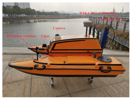
5.1. USV and Components

We apply the improved D* Lite to a real USV to verify the correctness and efficiency of the algorithm. The USV is a triple-hulled vessel with a size of 160 cm × 85 cm × 45 cm, which has been developed for water quality monitoring. It is powered by two propellers installed at the end of two floating vessels. During the navigation, the USV can obtain accurate GPS positions by the Real-Time Kinematic (RTK) GPS receiver. An electronic compass can detect the heading of the USV. A Lidar is deployed in the front of the USV, which can detect obstacles around the USV in real time within 20 m and return cloud points to identify the distance and the angle between the Lidar and the obstacles. An EXO sensor is installed at the end of the middle vessel to collect water quality parameters during the navigation. A camera on the top of the USV can transfer living video to users through 4G networks. There are two 12 V batteries in the floating vessels to provide power for the two propellers and all the electronic devices in the USV. We deploy the improved D* Lite algorithm in a Raspberry PI to control the autonomous navigation of the USV. The USV can also be remotely controlled by an Android-based app, which can be operated by the users. Figure 20 shows the USV and its components.

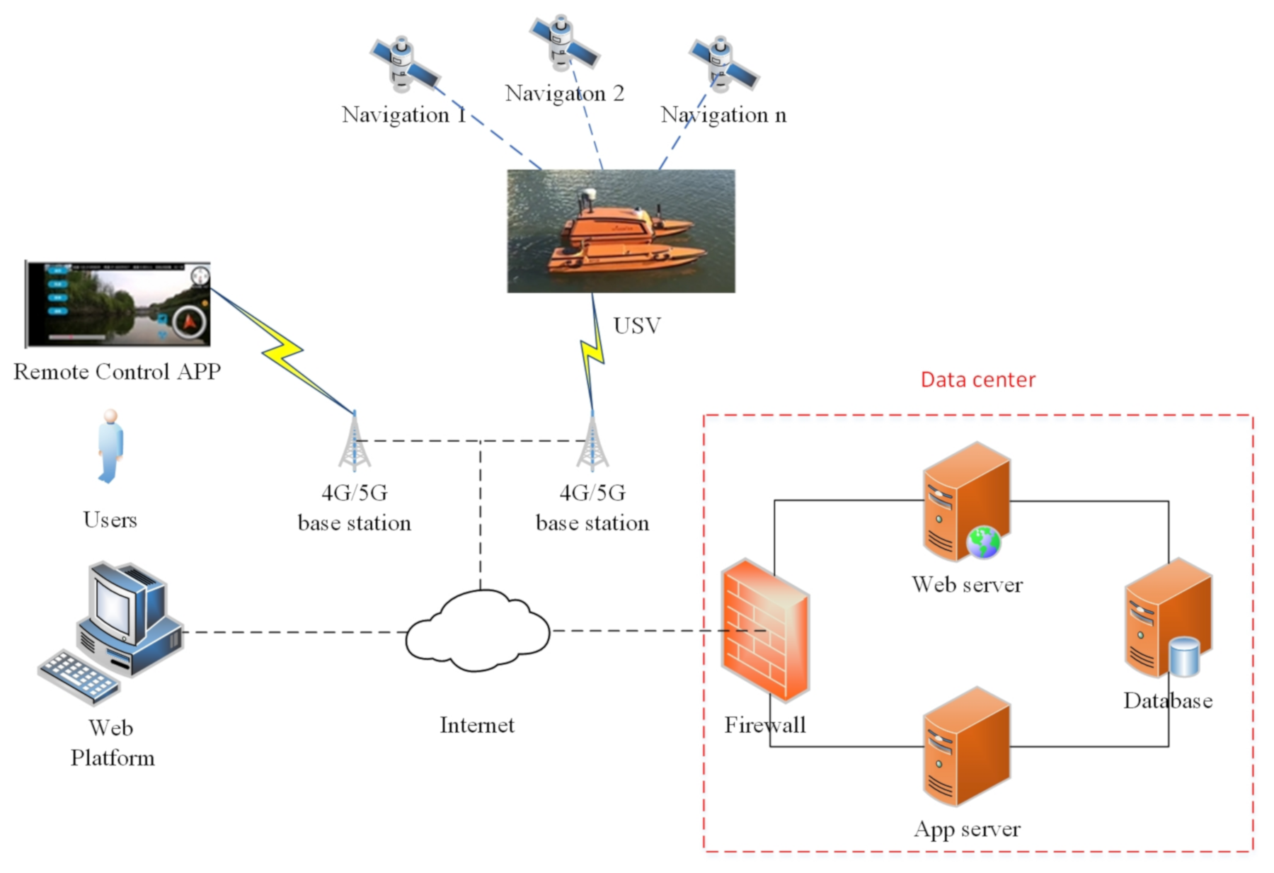
5.2. USV Communication Architecture

The communication architecture of the USV is shown in Figure 21. To create real-time communication connection between the USV and the remote-controlled app, a communication application is developed and deployed on an app server within a data center. All control commands can be transferred from the Android app to the USV in real time via the 4G/5G network and the communication application. All water quality and USV status data, such as GPS position, velocity and heading, are also transferred from the USV to the data center and the remote app via the communication application. In addition, users also can access the water quality data through a web platform deployed in the data center.

5.3. Safe Distance Test

The USV is tested in a small lake of approximately 104 × 140 square meters. We manually plan a path with four special goals for the USV on the Google Earth shown in Figure 22. The safe distance constant is set to 2 m, which means that the USV should keep at least 2 m away from obstacles during the autonomous navigation. In addition, we adjust the output power of the two propellers and set the USV’s velocity to 1 m/s.

We set the start waypoint at the north riverbank of the lake. There are steps down the north riverbank that allow us to launch the USV. We set the second waypoint ($Goal1$) in the middle of the lake and the third waypoint ($Goal2$) at the side of the west riverbank. From Figure 22, we find that there are no obstacles along the straight lines between the first three waypoints. Finally, we set the final waypoint at the northwest of the lake, resulting in a 220.52 m navigation path. There is a long riverbank composed of stones between the third waypoint ($Goal2$) and the final waypoint. The USV must avoid this huge obstacle (riverbank) and keep a safe distance to the riverbank during the navigation. In addition, there is a bridge across the river. The USV must pass through the bridge before it can reach the final waypoint. The purple dots in Figure 22 represent the actual path that the USV sails. We find that the USV moves along the riverbank with a safe distance. During the navigation, the live video is transferred from the camera on the USV to the app. Figure 23a shows a picture on the app that illustrates that the USV is moving along the west riverbank of the lake. Figure 23b shows that the USV is passing through the bridge to reach the final waypoint of the planned path. The USV’s GPS positions, speed and heading are all shown on the app. Users can also adjust the velocity by moving the slider on the bottom left of the screen. Furthermore, users can manually control the heading of the USV by changing the direction of the red arrow in the white circle. The Supplementary Videos (Video S2) show the entire procedure.

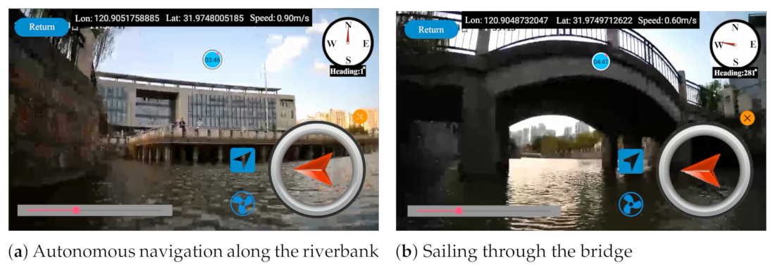
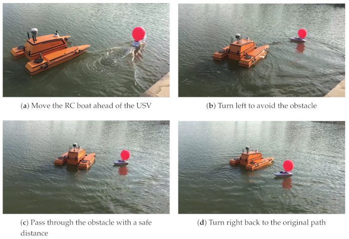
5.4. Dynamic Obstacle Avoidance

In this experiment, we bind a red balloon on a remote-controlled (RC) boat to simulate a dynamic obstacle. We plan a simple path with a straight line. When the USV is autonomously navigating according to the planned path, we remotely control the RC boat to move ahead to the USV (Figure 24a). The Lidar in the front of the USV detects the moving RC boat and a new path is planned immediately between its current position and the goal position. The USV turns the left according to the new path to avoid the RC boat (Figure 24b). Affected by the safe distance, the USV passes through the RC boat with a safe distance (Figure 24c). Finally, the USV turns right, returning to its original path (Figure 24d), and continues its autonomous navigation. The Supplementary Videos (Video S1) show the entire procedure.

6. Conclusions

We have improved the traditional D* Lite algorithm and realized multi-goal path planning and obstacle avoidance for USVs in unknown, dynamic and complex environments. By expanding the algorithm to search more neighbor nodes and increasing the safe distance, we have solved the issue of the limited steering maneuverability of USVs during autonomous navigation. A path optimization algorithm has been proposed to eliminate sharp turns and reduce the path length. The minimum binary heap has been used to optimize the priority queue of the D* Lite to reduce the path planning time and improve the search efficiency. Experimental results show that the improved D* Lite has much better path planning performance and is more realistic in practice.

In the future, we will further test and improve the stability and efficiency of the improved D* Lite with other obstacle detection sensors such as a stereo camera and millimeter-wave radar to further enhance the USV.

References

1. Glasgow, H.B.; Burkholder, J.M.; Reed, R.E.; Lewitus, A.J.; Kleinman, J.E. Real-time remote monitoring of water quality: A review of current applications, and advancements in sensor, telemetry, and computing technologies. J. Exp. Mar. Biol. Ecol. 2004, 300, 409–448. [Google Scholar] [CrossRef]
2. Liu, Z.; Zhang, Y.; Yu, X.; Yuan, C. Unmanned surface vehicles: An overview of developments and challenges. Annu. Rev. Control 2016, 41, 71–93. [Google Scholar] [CrossRef]
3. Li, Z.; Bachmayer, R.; Vardy, A. Vector field path following control for unmanned surface vehicles. In Proceedings of the OCEANS 2017-Aberdeen, Aberdeen, UK, 19–22 June 2017; pp. 1–9. [Google Scholar]
4. Singh, Y.; Sharma, S.; Sutton, R.; Hatton, D.; Khan, A. A constrained A* approach towards optimal path planning for an unmanned surface vehicle in a maritime environment containing dynamic obstacles and ocean currents. Ocean Eng. 2018, 168, 187–201. [Google Scholar] [CrossRef] [Green Version]
5. Zhang, R.; Tang, P.; Su, Y.; Li, X.; Yang, G.; Shi, C. An adaptive obstacle avoidance algorithm for unmanned surface vehicle in complicated marine environments. IEEE/CAA J. Autom. Sin. 2014, 1, 385–396. [Google Scholar]
6. Shu-Xi, W. The improved dijkstra’s shortest path algorithm and its application. Procedia Eng. 2012, 29, 1186–1190. [Google Scholar] [CrossRef] [Green Version]
7. Chao, N.; Liu, Y.K.; Xia, H.; Peng, M.J.; Ayodeji, A. DL-RRT* algorithm for least dose path Re-planning in dynamic radioactive environments. Nucl. Eng. Technol. 2019, 51, 825–836. [Google Scholar] [CrossRef]
8. Hart, P.E.; Nilsson, N.J.; Raphael, B. A formal basis for the heuristic determination of minimum cost paths. IEEE Trans. Syst. Sci. Cybern. 1968, 4, 100–107. [Google Scholar] [CrossRef]
9. Cabreira, T.M.; Brisolara, L.B.; Ferreira, P.R., Jr. Survey on coverage path planning with unmanned aerial vehicles. Drones 2019, 3, 4. [Google Scholar] [CrossRef] [Green Version]
10. Kumar Das, P.; Patro, S.N.; Panda, C.N.; Balabantaray, B. D* lite algorithm based path planning of mobile robot in static Environment. Int. J. Comput. Commun. Technol. (IJCCT) 2011, 2, 32–36. [Google Scholar]
11. Stentz, A. The D* Algorithm for Real-Time Planning of Optimal Traverses; Technical Report; Robotics Institute, Carnegie Mellon University: Pittsburgh, PA, USA, 1994. [Google Scholar]
12. Stentz, A. The focussed dˆ* algorithm for real-time replanning. In Proceedings of the International Joint Conference on Artificial Intelligence, Montreal, QC, Canada, 20–25 August 1995; Volume 95, pp. 1652–1659. [Google Scholar]
13. Lei, Q.; Hui, Z. Implementation of Path Finding on 2D Game Maps. J. Hum. Univ. Technol. 2012, 1, 66–69. [Google Scholar]
14. Guo, J.; Liu, L.; Liu, Q.; Qu, Y. An Improvement of D* Algorithm for Mobile Robot Path Planning in Partial Unknown Environment. In Proceedings of the 2009 Second International Conference on Intelligent Computation Technology and Automation, Changsha, China, 16 October 2009; Volume 3, pp. 394–397. [Google Scholar] [CrossRef]
15. Yan, B.; Chen, T.; Zhu, X.; Yue, Y.; Xu, B.; Shi, K. A Comprehensive Survey and Analysis on Path Planning Algorithms and Heuristic Functions. In Proceedings of the Science and Information Conference, London, UK, 16–17 July 2020; pp. 581–598. [Google Scholar]
16. Likhachev, M.; Koenig, S. A Generalized Framework for Lifelong Planning A* Search. In Proceedings of the Fifteenth International Conference on Automated Planning and Scheduling (ICAPS 2005), Monterey, QC, USA, 5–10 June 2005; pp. 99–108. [Google Scholar]
17. Ferguson, D.; Stentz, A. Field D*: An interpolation-based path planner and replanner. In Robotics Research; Springer: Berlin/Heidelberg, Germany, 2007; pp. 239–253. [Google Scholar]
18. Koenig, S.; Likhachev, M. Dˆ* lite. In Proceedings of the AAAI Conference on Artificial Intelligence, Edmonton, AB, Canada, 28 July– 1August 2002; pp. 476–483. [Google Scholar]
19. Koenig, S.; Likhachev, M. Fast replanning for navigation in unknown terrain. IEEE Trans. Robot. 2005, 21, 354–363. [Google Scholar] [CrossRef]
20. Oral, T.; Polat, F. A multi-objective incremental path planning algorithm for mobile agents. In Proceedings of the 2012 IEEE/WIC/ACM International Conferences on Web Intelligence and Intelligent Agent Technology, Macau, China, 4–7 December 2012; Volume 2, pp. 401–408. [Google Scholar]
21. Ferguson, D.; Stentz, A. The delayed D* algorithm for efficient path replanning. In Proceedings of the 2005 IEEE International Conference on Robotics and Automation, Barcelona, Spain, 18–22 April 2005; pp. 2045–2050. [Google Scholar]
22. Al-Mutib, K.; AlSulaiman, M.; Emaduddin, M.; Ramdane, H.; Mattar, E. D* lite based real-time multi-agent path planning in dynamic environments. In Proceedings of the 2011 Third International Conference on Computational Intelligence, Modelling & Simulation, Langkawi, Malaysia, 20–22 September 2011; pp. 170–174. [Google Scholar]
23. Yu, J.; Liu, G.; Zhao, Z.; Wang, X.; Xu, J.; Bai, Y. Improved D* Lite algorithm path planning in complex environment. In Proceedings of the 2020 Chinese Automation Congress (CAC), Shanghai, China, 6–8 November 2020; pp. 2226–2230. [Google Scholar]
24. Yue, W.; Franco, J.; Cao, W.; Yue, H. ID* Lite: Improved D* Lite algorithm. In Proceedings of the 2011 ACM Symposium on Applied Computing, TaiChung, Taiwan, 21–24 March 2011; pp. 1364–1369. [Google Scholar]
25. Yun, S.C.; Ganapathy, V.; Chien, T.W. Enhanced D* Lite Algorithm for mobile robot navigation. In Proceedings of the 2010 IEEE Symposium on Industrial Electronics and Applications (ISIEA), Penang, Malaysia, 3–5 October 2010; pp. 545–550. [Google Scholar]
26. Le, A.T.; Bui, M.Q.; Le, T.D.; Peter, N. D* Lite with Reset: Improved Version of D* Lite for Complex Environment. In Proceedings of the IEEE International Conference on Robotic Computing, Taichung, Taiwan, 10–12 April 2017. [Google Scholar]
27. Barma, P.S.; Dutta, J.; Mukherjee, A. A 2-opt guided discrete antlion optimization algorithm for multi-depot vehicle routing problem. Decis. Mak. Appl. Manag. Eng. 2019, 2, 112–125. [Google Scholar]
28. Ravankar, A.; Ravankar, A.A.; Kobayashi, Y.; Hoshino, Y.; Peng, C.C. Path smoothing techniques in robot navigation: State-of-the-art, current and future challenges. Sensors 2018, 18, 3170. [Google Scholar] [CrossRef] [PubMed] [Green Version]
29. Zagradjanin, N.; Pamucar, D.; Jovanovic, K. Cloud-based multi-robot path planning in complex and crowded environment with multi-criteria decision making using full consistency method. Symmetry 2019, 11, 1241. [Google Scholar] [CrossRef] [Green Version]
30. Edelkamp, S.; Elmasry, A.; Katajainen, J. Optimizing binary heaps. Theory Comput. Syst. 2017, 61, 606–636. [Google Scholar] [CrossRef]
31. Yang, L.; Qi, J.; Song, D.; Xiao, J.; Han, J.; Xia, Y. Survey of robot 3D path planning algorithms. J. Control. Sci. Eng. 2016, 2016, 7426913. [Google Scholar] [CrossRef] [Green Version]
Figure 1. Adjacent nodes for search.
Applsci 11 07863 g001
Figure 2. USV heading and steering angle.
Applsci 11 07863 g002
Figure 3. Next position calculation with steering angle limitation.
Applsci 11 07863 g003
Figure 4. Path planned by D* Lite.
Applsci 11 07863 g004
Figure 5. Procedure of path planning and optimization.
Applsci 11 07863 g005
Figure 6. Data storage of binary heap.
Applsci 11 07863 g006
Figure 7. Procedure of multi-goal path planning in unknown environments.
Applsci 11 07863 g007
Figure 8. Path planned on 400 × 400 map.
Applsci 11 07863 g008
Figure 9. Path planning on 200 × 200 map.
Applsci 11 07863 g009
Figure 10. Path planning on 400 × 400 map.
Applsci 11 07863 g010
Figure 11. Path optimization on 200 × 200 map.
Applsci 11 07863 g011
Figure 12. Path optimization on 400 × 400 map.
Applsci 11 07863 g012
Figure 13. Comparison of path length.
Applsci 11 07863 g013
Figure 14. Efficiency evaluation of minimum binary heap.
Applsci 11 07863 g014
Figure 15. Multi-goal path planning in a static environment.
Applsci 11 07863 g015
Figure 16. Multi-goal path planning in a dynamic environment.
Applsci 11 07863 g016
Figure 17. Detection range in unknown environments.
Applsci 11 07863 g017
Figure 18. Local path planned in local environment.
Applsci 11 07863 g018aApplsci 11 07863 g018b
Figure 19. Full path planed in unknown environment.
Applsci 11 07863 g019
Figure 20. USV and components.
Applsci 11 07863 g020
Figure 21. Communication architecture of USV.
Applsci 11 07863 g021
Figure 22. Planned and actual path.
Applsci 11 07863 g022
Figure 23. Live video from the USV.
Applsci 11 07863 g023
Figure 24. Procedure of dynamic obstacle avoidance.
Applsci 11 07863 g024