Deep Neural Fuzzy System Oriented toward High-Dimensional Data and Interpretable Artificial Intelligence

Abstract

Fuzzy systems (FSs) are popular and interpretable machine learning methods, represented by the adaptive neuro-fuzzy inference system (ANFIS). However, they have difficulty dealing with high-dimensional data due to the curse of dimensionality. To effectively handle high-dimensional data and ensure optimal performance, this paper presents a deep neural fuzzy system (DNFS) based on the subtractive clustering-based ANFIS (SC-ANFIS). Inspired by deep learning, the SC-ANFIS is proposed and adopted as a submodule to construct the DNFS in a bottom-up way. Through the ensemble learning and hierarchical learning of submodules, DNFS can not only achieve faster convergence, but also complete the computation in a reasonable time with high accuracy and interpretability. By adjusting the deep structure and the parameters of the DNFS, the performance can be improved further. This paper also performed a profound study of the structure and the combination of the submodule inputs for the DNFS. Experimental results on five regression datasets with various dimensionality demonstrated that the proposed DNFS can not only solve the curse of dimensionality, but also achieve higher accuracy, less complexity, and better interpretability than previous FSs. The superiority of the DNFS is also validated over other recent algorithms especially when the dimensionality of the data is higher. Furthermore, the DNFS built with five inputs for each submodule and two inputs shared between adjacent submodules had the best performance. The performance of the DNFS can be improved by distributing the features with high correlation with the output to each submodule. Given the results of the current study, it is expected that the DNFS will be used to solve general high-dimensional regression problems efficiently with high accuracy and better interpretability.

1. Introduction

Fuzzy systems (FSs) originated from the fuzzy set theory proposed by Zadeh in 1965 [1], which are based on fuzzy rules. FSs are more interpretable and intuitive methods that can match any set of input–output data by each fuzzy rule [2]. As soft computing techniques, FSs have achieved great success in dealing with numerous problems of uncertainty, such as the seismic vulnerability assessment of buildings [3,4,5], the prediction of the irrigation water infiltration rate [6], the automatic classification of crop disease images [7], etc.

However, there are three main challenges in developing optimal FSs through the analysis of the research status: (1) Optimization: Optimizing FSs within a valid period of time to achieve higher accuracy and faster convergence is now worthy of in-depth study, which is also challenging. (2) The curse of dimensionality: The number of fuzzy rules increases exponentially with the dimensionality of the input, which leads to the computation not being able to be completed within a reasonable time. Hence, it is difficult for FSs to deal with high-dimensional problems. (3) Interpretability: The interpretability is the advantage of FSs that distinguishes them from other machine learning models. However, as the number of fuzzy rules increases, the interpretability of FSs will be affected. Therefore, how to solve the high-dimensional problem on the basis of ensuring better interpretability is one of the current bottlenecks.

In recent years, great efforts have been made to improve FSs [8]. Evolutionary algorithms (EAs) [9,10], the gradient descent (GD) algorithm [11], and GD plus least squares estimation (LSE) [12] have been proposed to optimize FSs. Although EAs can search for the optimal solution with enough iterations, the computational cost is too expensive to be suitable for the optimization of FSs. The adaptive neuro-fuzzy inference system (ANFIS) proposed by Jang formed by GD plus LSE [12] has been widely applied in national energy demand forecasting [13,14], flood sensitivity forecasting [15], geographic temperature forecasting [16], heart disease classification [17], and so on. However, the convergence speed of GD or GD plus LSE is very slow, and they easily fall into local optimal solutions.

In view of the above problems, new techniques based on the ANFIS optimized by EAs have been emerging. For example, Azar et al. proposed the improved ANFIS based on the Harris hawks optimization evolutionary algorithm and demonstrated its effectiveness on the prediction of the longitudinal dispersion coefficient of natural rivers [18]. Xu et al. proposed an ANFIS-PSO method based on an improved particle swarm optimization algorithm and successfully applied it to the evaluation of tool wear [19]. Kaur et al. combined the genetic algorithm with the ANFIS to further improve the prediction accuracy of the waterborne disease cholera [20]. In addition, a method of optimizing the ANFIS based on an improved firefly algorithm and the differential evolution optimization algorithm was proposed by Balasubramanian [21], which has been proven to be effective in the application of medical disease prediction. Ehteram et al. used three optimization algorithms (sine–cosine algorithm, particle swarm optimization algorithm, and firefly algorithm) to optimize the ANFIS to improve the prediction accuracy [22]. However, all the above methods only focus on the optimization of FSs and still have challenges in solving high-dimensional data.

In order to enable FSs to process high-dimensional data, principal component analysis (PCA) [23] is widely used for dimensionality reduction. Razin et al. combined the ANFIS with PCA to predict the Iranian ionospheric time series, which can shorten the convergence time and obtain the optimal solution [24]. Phan et al. solved the problem of predicting the fracture pressure of defective pipelines more effectively through the combination of PCA and the ANFIS [25]. Meanwhile, it is worth referring to the efficient training algorithm named MBGD-RDA proposed by Wu et al. for TSK FSs in 2020 [26]. PCA was applied to constrain the maximum input dimensionality to five, and several novel techniques were proposed in MBGD-RDA. However, in terms of the above methods, the performance will be affected due to the loss of important features by PCA, especially for high-dimensional data. Therefore, the curse of dimensionality has not been fundamentally solved for FSs.

The primary target of this study was to enable FSs to effectively solve high-dimensional regression problems on the basis of ensuring the performance and interpretability. The main contributions of this paper are as follows:

(1)

Inspired by deep learning, the subtractive clustering-based ANFIS (SC-ANFIS) is proposed and adopted as a submodule to construct the deep neural fuzzy system (DNFS) in a bottom-up way;

(2)

Combined with ensemble learning and hierarchical learning, the DNFS that can solve general high-dimensional regression problems efficiently with high accuracy and interpretability is proposed;

(3)

The effect of the deep structure and the combination of submodule inputs on the performance of the DNFS are researched in-depth;

(4)

The effectiveness and superiority of the DNFS are validated on five real-world datasets with various dimensionalities.

The remainder of this paper is organized as follows: Section 2 introduces the proposed DNFS algorithm. Section 3 describes the datasets and performance indices used in the experiments. Section 4 presents the experimental results to verify the effectiveness of the DNFS. Section 5 draws the conclusion and points out the directions for future research.

2. The DNFS Algorithm

2.1. The SC-ANFIS Submodel

The structure of the ANFIS is composed of an adaptive neural network and an FS. It not only inherits the adaptive learning ability of neural networks, but also keeps the interpretability of FSs. The ANFIS can adjust the parameters according to prior knowledge so that the predicted values are closer to the target values, which has achieved great success in many applications [27]. The SC-ANFIS is proposed in this paper, which applies subtractive clustering (SC) to construct a Sugeno fuzzy inference system in the ANFIS. The SC-ANFIS can effectively avoid the combinatorial explosion of fuzzy rules when the dimensionality of the input is very high. In addition, the fuzzy rules generated by SC are more consistent with the data than those obtained without clustering. The input space can be divided appropriately, and the number of membership functions (MFs) and the parameters for each input domain can be reasonably determined [28]. There are two other well-known methods to construct fuzzy inference systems: (1) grid partitioning; (2) fuzzy c-means clustering [29]. It has been proven that SC is better than other algorithms [30,31], and it was adopted as the method to generate the fuzzy inference system in the ANFIS.

There are several types of MFs in the ANFIS (e.g., triangular, trapezoidal, generalized bell, Gaussian, etc.) that can be applied [32]. The MF used in the SC-ANFIS is Gaussian, considering that it has the advantages of being nonzero, simple, and smooth and having fewer parameters compared with other MFs [33]. Furthermore, relevant studies have demonstrated that the performance of the Gaussian MF is better than others in many nonlinear complex problems [34,35]. The general ANFIS structure, which has five layers and two inputs, is as follows:

Layer 1: Calculate the MF values for each input domain.

$$\begin{array}{c}\hfill O_1^i=u_{A_i}\left(x_1\right),i=1,2\mid O_1^i=u_{B_{(i-2)}}\left(x_2\right),i=3,4\end{array}$$

(1)

where $x_1,x_2$ are the inputs and $u_{A_i}\left(x\right)$ and $u_{B_{(i-2)}}\left(x\right)$ are the corresponding MF values, which can be expressed in the Equation (2).

$$\begin{array}{c}\hfill u_{A_i}\left(x_1\right)=u_{B_i}\left(x_2\right)=e^{-\frac{{(x-c_i)}^2}{2{\sigma }_i^2}},i=1,2\end{array}$$

(2)

where $c_i$ and ${\sigma }_i$ are the parameters of the Gaussian MF that result in the different shapes of the MF for each input;

Layer 2: Multiply the MF values of the inputs as the excitation intensity corresponding to the fuzzy rule:

$$O_2^i=w_i=u_{A_i}\left(x_1\right) \times u_{B_i}\left(x_2\right),i=1,2;$$

(3)

Layer 3: Normalize the incentive intensity of the fuzzy rule, which represents the weight of the rule in all rule bases:

$$O_3^i={\overline{w}}_i=\frac{w_i}{w_1+w_2},i=1,2;$$

(4)

Layer 4: Calculate the output of each fuzzy rule:

$$O_4^i={\overline{w}}_i{f}_i={\overline{w}}_i\left(p{x}_1+q{x}_2+r\right),i=1,2$$

(5)

where $\left\{p,q,r\right\}$ are the consequent parameters for each fuzzy rule;

Layer 5: Integrate the output of all fuzzy rules and calculate the final output.

$$O_5^1=\sum _i{\overline{w}}_i{f}_i,i=1,2$$

(6)

where $O_k^i$ is the output of the k-th layer.

2.2. The Structure of the DNFS Algorithm

This paper employed the SC-ANFIS as a submodule to construct the DNFS. By dividing the high-dimensional data into several groups of m-dimensionality, the results are obtained by each submodule in a more efficient way.

The number of inputs for each submodule (m) and the number of inputs shared between adjacent submodules (n) need to be initialized, so as to construct DNFSm-n. Figure 1 shows the general structure diagram of DNFS5-2.

The basic definition of the structure of DNFSm-n is defined as follows:

Layer 1: The number of inputs for each submodules is m, and n inputs are shared between adjacent submodules. Each submodule works separately and obtains its own results;

Layer 2: The outputs of each submodules in the first layer are merged into a new dataset, which are applied in the second layer. The way of grouping the inputs is the same as the first layer;

Similarly, the inputs of layer L consist of the outputs of each submodule of L-1. The submodules are built in the same way as the first layer to group the inputs. The submodules of each layer are built bottom-up until the inputs of the last layer are only enough to build one submodule, and the final result is obtained.

2.3. The Implementation Steps of the DNFS Algorithm

This section mainly introduces the implementation steps of the DNFS algorithm. The flowchart of the proposed DNFSm-n is shown in Figure 2. The execution process of DNFSm-n is as follows:

Step 1. Data preprocessing: Each numerical feature was mapminmax-normalized, and the dataset was divided into a training set and a test set;

Step 2. Define the structure of the DNFS: Determine m, n, the layers, and the number of submodules of each layer;

Step 3. Group the training set and the test set: The training set and the test set are divided into several groups of m-dimensionality, and each group corresponds to one submodule;

Step 4. Training submodule: Traverse each submodule of the current layer, and put the grouped training set into the corresponding submodule for training;

Step 5. Test submodule: Put the grouped test set into the corresponding submodule, which has been trained to perform the testing;

Step 6. Determine if the DNFS is completed: If the current layer is the last one of the DNFS structure, the current outputs are directly taken as the final output, and turn to Step 7. Otherwise, the outputs of the current layer are merged into a new dataset, which are adopted as the inputs of the next layer, and return to Step 3;

Step 7. Obtain the final result.

There is a special case in Step 3: the group needs to be supplemented if there are not enough features in the grouping to constitute m-dimensional inputs. The main situations are as follows:

• If this happens when the training set and the test set are grouped in the first layer, the features are selected in turn from the first group that has been divided to supplement them;
• If this happens when the training set and the test set are grouped among the second layer to the last layer, all the outputs of the upper layer are sorted based on the error value in ascending order, and the outputs with the smallest error are selected according to the number of missing ones.

3. Dataset and Performance Index

3.1. The Datasets

To demonstrate that the proposed DNFS can effectively solve the high-dimensional regression problems, this paper selected five representative datasets with various dimensionality from the UCI machine learning repository, and the specific information of the datasets is shown in

Table 1. Summary of the five regression datasets.

Index	Dataset	No. of Features	No. of Samples	Application Field
1	Parkinson’s 1	21	5875	Parkinson’s telemonitoring
2	Wdbc 2	30	569	Breast cancer diagnosis
3	Superconductor 3	81	10,000	Superconductor temperature prediction
4	Music 4	69	1059	Geographic origin of music
5	Residential Building 5	108	372	Residential building cost

¹http://archive.ics.uci.edu/ml/datasets/Parkinsons+Telemonitoring (accessed on 20 March 2021); ² http://archive.ics.uci.edu/ml/datasets/Breast+Cancer+Wisconsin+%28Prognostic%29 (accessed on 20 March 2021); ³ http://archive.ics.uci.edu/ml/datasets/Superconductivty+Data (accessed on 20 March 2021); ⁴ http://archive.ics.uci.edu/ml/datasets/Geographical+Original+of+Music (accessed on 20 March 2021); ⁵ http://archive.ics.uci.edu/ml/datasets/Residential+Building+Data+Set (accessed on 20 March 2021).

. Sixty percent of the samples were randomly selected for training and the remaining forty percent for testing.

3.2. Performance Index

To evaluate the performance of the DNFS algorithm comprehensively, four performance indices (e.g., mean absolute error (MAE), root mean squared error (RMSE), Akaike information criterion (AIC) [36], and symmetric mean absolute percentage error (SMAPE)) were introduced. MAE, RMSE, and SMAPE mainly measure the precision, while AIC considers the precision and simplicity simultaneously [37]. They are defined as:

$$\begin{array}{c}\hfill \mathit{MAE}=\frac{1}{n}\sum _{i=1}^n\left|{\hat{y}}_i-y_i\right|\end{array}$$

(7)

$$\begin{array}{c}\hfill \mathit{RMSE}=\sqrt{\left(\frac{1}{n}\sum _{i=1}^n{\left({\hat{y}}_i-y_i\right)}^2\right)}\end{array}$$

(8)

$$\begin{array}{c}\hfill \mathit{AIC}=nlog{\left(RMSE\right)}^2+2k\end{array}$$

(9)

$$\begin{array}{c}\hfill \mathit{SMAPE}=\frac{100\%}{n}\sum _{i=1}^n\frac{2\left|{\hat{y}}_i-y_i\right|}{\left(\left|{\hat{y}}_i\right|+\left|y_i\right|\right)}\end{array}$$

(10)

where n is the number of samples, $\hat{y}$ and y are the predicted value and the true value, respectively, and k is the number of parameters that can be optimized. The parameters of a submodule are equal to the number of antecedent parameters ($A\ast T\ast S$) plus the number of consequent parameters ($R\ast (S+1)$). A and T are the number of MF parameters and the MF in each input domain, respectively. S is the input dimensions. R is the number of fuzzy rules ($T^S$). The parameters of the DNFS are equal to the sum of the parameters of each submodule.

In order to reflect the comprehensive performance of the model, this paper also defined an evaluation method to rank each index. The final score was the sum of the scores of each index. The experimental platform of this paper was a desktop computer running MATLAB 2020a and Windows 10 Education 64x, with Intel Core i7-9700 CPU @ 3.00 GHz, 16 GB memory, and a 512 GB solid state drive.

4. Experimental Results

4.1. The Effect of the Number of Submodule Inputs on the DNFS

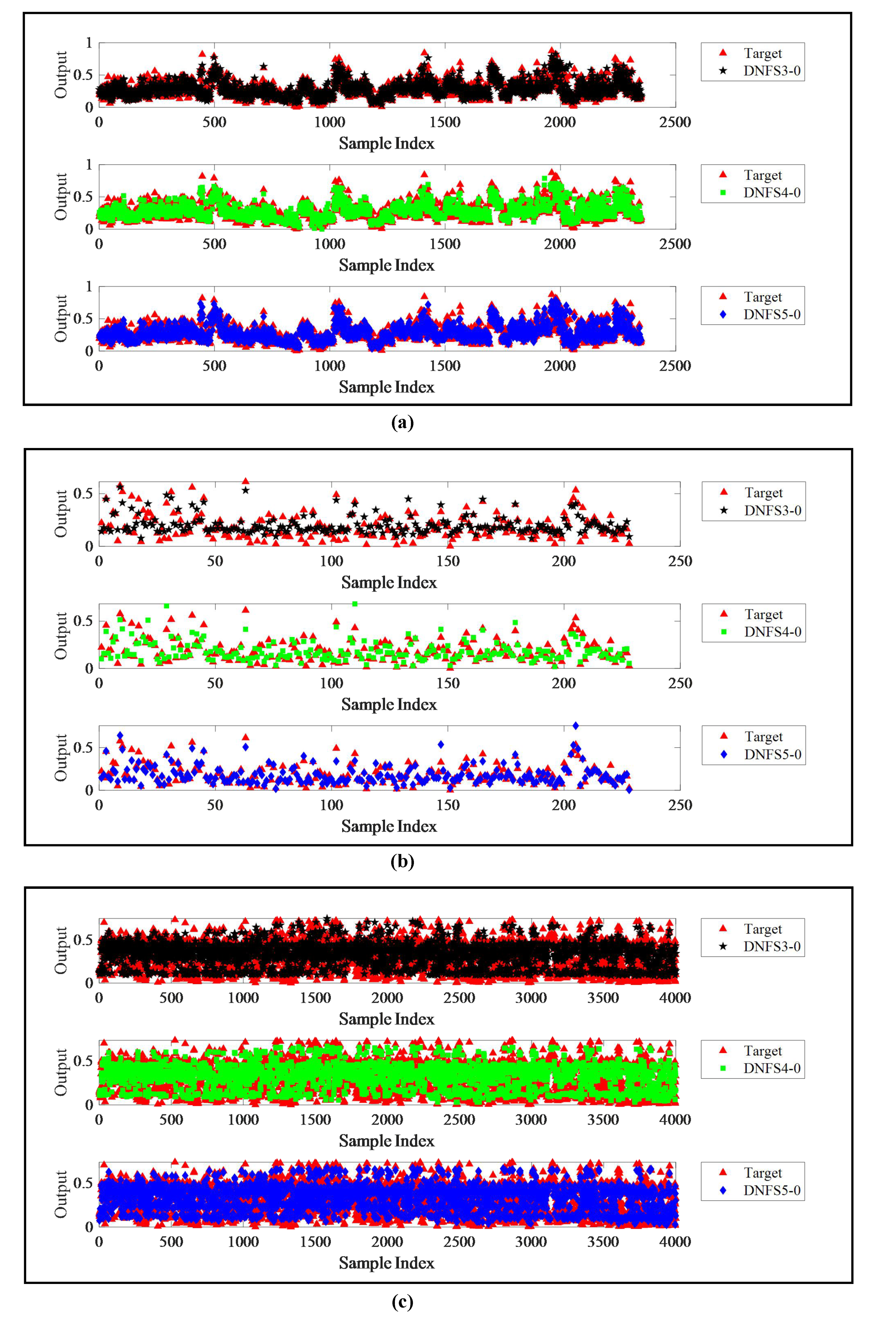
This section mainly focuses on the effect of the number of submodule inputs on the DNFS for the first three datasets. The corresponding DNFSs with 3, 4, and 5 submodule inputs are DNFS3-0, DNFS4-0, and DNFS5-0, respectively.

The performance comparison of DNFSs with different submodule inputs on the first three test datasets are shown in

Table 2. The performance of DNFSs with different submodule inputs on Test Dataset No. 1.

Methods	AIC	MAE	RMSE	SMAPE	Score	Layers	No. of Submodules	No. of Params	Time (s)
DNFS3-0	−12,986.28	0.039451	0.051882	4.0123%	9	3	11	460	14.4406
DNFS4-0	−12,020.87	0.039588	0.052901	4.0713%	5	3	9	897	30.1497
DNFS5-0	−10,667.72	0.037904	0.051602	3.8449%	10	2	6	1632	96.9152

,

Table 3. The performance of DNFSs with different submodule inputs on Test Dataset No. 2.

Methods	AIC	MAE	RMSE	SMAPE	Score	Layers	No. of Submodules	No. of Params	Time (s)
DNFS3-0	−480.23	0.047057	0.057765	7.8493%	7	4	17	410	2.2976
DNFS4-0	−372.59	0.042295	0.060043	6.1742%	6	3	11	455	1.3916
DNFS5-0	−409.42	0.035025	0.049632	5.4848%	11	3	9	480	1.3602

and

Table 4. The performance of DNFSs with different submodule inputs on Test Dataset No. 3.

Methods	AIC	MAE	RMSE	SMAPE	Score	Layers	No. of Submodules	No. of Params	Time (s)
DNFS3-0	−14,625.26	0.081153	0.105330	8.1929%	5	4	40	1690	76.9161
DNFS4-0	−14,451.25	0.078638	0.101860	7.8498%	7	4	30	1911	77.8035
DNFS5-0	−14,761.41	0.073618	0.098158	7.5000%	12	3	22	1904	76.7091

. The prediction charts performed by the three DNFSs on the first three test datasets are shown in Figure 3. The analysis of the results obtained was as follows:

DNFS5-0 outperformed DNFS3-0 and DNFS4-0 in the prediction accuracy, which determined that its comprehensive score was always the highest among the three cases. The MAE, RMSE, and SMAPE of DNFS5-0 were smaller than the other two algorithms on the three datasets. As shown in Figure 3, it also can be seen that DNFS5-0 achieved the best fitting effect, while the other two algorithms performed relatively poor.

In terms of model complexity, DNFS5-0 had the minimum layers and submodules, followed by DNFS4-0 and DNFS3-0. It can be concluded that more submodules and layers needed to be built to decompose the high-dimensional data with fewer submodule inputs. Meanwhile, DNFS5-0 had the most parameters and DNFS3-0 the least on average. The AIC of DNFS3-0 was the minimum for the first two datasets, while DNFS5-0 obtained the best AIC on Dataset No. 3.

The average computational time that DNFS3-0, DNFS4-0, and DNFS5-0 spent on the three datasets was 31.21 s, 36.44 s, and 58.32 s respectively. It can be concluded that DNFS3-0 is the most efficient method for the three cases.

Based on the analysis above, DNFS5-0 can ensure the optimal performance with less complexity. The advantage of DNFS5-0 was further revealed with the increase of dimensionality, by which the high-dimensional data could be divided into submodules more rapidly. Therefore, the DNFS algorithm with five submodule inputs was researched further.

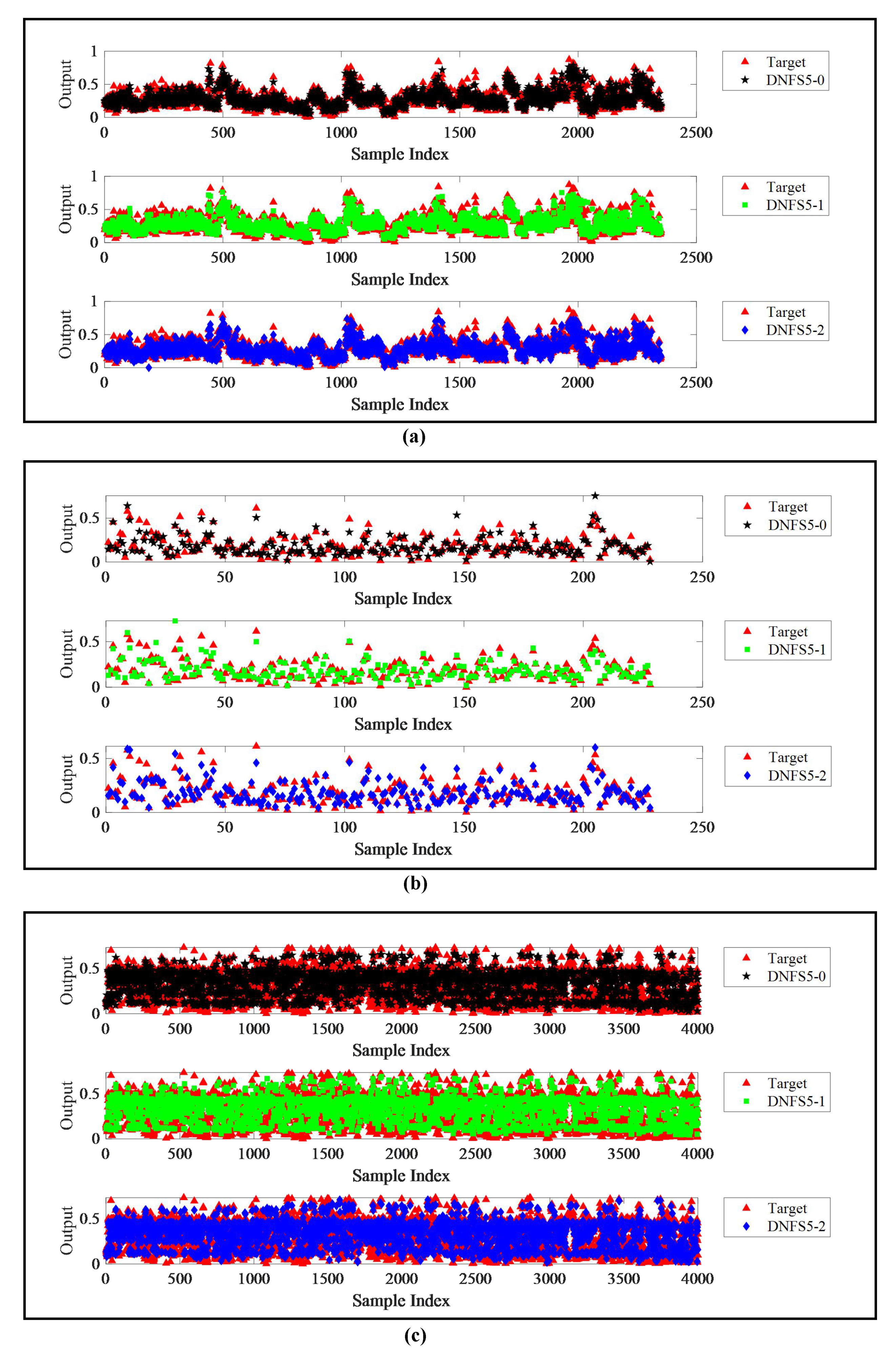
4.2. The Effect of the Number of Inputs Shared by Adjacent Submodules on the DNFS

The target of this section is to explore the performance of the DNFS with different shared inputs on the first three datasets.

As shown in

Table 5. The performance of DNFSs with different shared inputs on Test Dataset No. 1.

Methods	AIC	MAE	RMSE	SMAPE	Score	Layers	No. of Submodules	No. of Params	Time (s)
DNFS5-0	−10,667.72	0.037904	0.051602	3.8449%	7	2	6	1632	99.3428
DNFS5-1	−11,899.62	0.039198	0.051779	4.0155%	6	2	6	1008	56.0007
DNFS5-2	−10,960.29	0.036194	0.048819	3.6826%	11	3	10	1616	75.7929

,

Table 6. The performance of DNFSs with different shared inputs on Test Dataset No. 2.

Methods	AIC	MAE	RMSE	SMAPE	Score	Layers	No. of Submodules	No. of Params	Time (s)
DNFS5-0	−409.42	0.035025	0.049632	5.4848%	9	3	9	480	2.1238
DNFS5-1	−84.53	0.036351	0.053814	5.5005%	5	3	11	624	1.7390
DNFS5-2	97.92	0.034611	0.045798	5.4495%	10	3	14	752	2.1080

and

Table 7. The performance of DNFSs with different shared inputs on Test Dataset No. 3.

Methods	AIC	MAE	RMSE	SMAPE	Score	Layers	No. of Submodules	No. of Params	Time (s)
DNFS5-0	−14,761.41	0.073618	0.098158	7.5000%	9	3	22	1904	78.6101
DNFS5-1	−14,065.16	0.074622	0.098456	7.6021%	5	3	26	2240	92.0680
DNFS5-2	−12,060.34	0.072505	0.096758	7.4269%	10	4	40	3312	134.6429

, DNFS5-2 had the minimum MAE, RMSE, and SMAPE on the three test datasets, which indicated that the best prediction accuracy can be achieved by DNFS5-2. As shown in Figure 4, it can be seen obviously that DNFS5-2 achieved the best fitting effect on the three test datasets among the three cases.

Based on the experimental results obtained, it also can be found that the structures of DNFS5-0 and DNFS5-1 were simpler than DNFS5-2. There is no doubt that the more shared inputs there are, the more layers and submodules will be under the same submodule inputs. Consequently, DNFS5-2 had the most layers, submodules, and parameters on average, which led to its poor AIC value.

On average, DNFS5-0, DNFS5-1, and DNFS5-2 spent 60.02 s, 49.93 s, and 70.84 s on the three test datasets. Therefore, DNFS5-1 is the most efficient method, followed by DNFS5-0 and DNFS5-2.

As the comprehensive performance was taken into consideration, the superiority of DNFS5-2 is shown obviously. The score of DNFS5-2 was the highest among the three DNFSs, which can resolve the high-dimensional data within a valid period of time. On the whole, DNFS without shared input had a simpler structure, and that with two shared inputs had better prediction accuracy.

4.3. The Effect of the Combination of Submodule Inputs on the DNFS

To reveal the effect of the combination of submodule inputs on the DNFS, this paper introduced DNFS5-2-Random. The implementation steps of DNFS5-2-Random are as follows: each time DNFS5-2 is executed, the input of each layer is randomly scrambled. After DNFS5-2 is executed in this way 10 times, the optimal input order is taken as the final order of DNFS5-2, and the corresponding results are obtained.

Meanwhile, in order to validate the effectiveness and superiority of DNFS, MBGD-RDA, which is the latest training algorithm for TSK FSs, was introduced to be compared with DNFS. MBGD-RDA was implemented by the MATLAB implementation given in [26], and its initial learning parameters were consistent with [26], which proved to be the optimal one. Besides, the radial basis function (RBF) [38], generalized regression neural network (GRNN) [39], and long-short term memory (LSTM) [40] were also introduced to further reveal the superiority of the DNFS, which represent general machine learning models. Their implementation were mainly realized by calling the newrb, newgrnn, and trainNetwork functions of the deep learning toolbox in MATLAB 2020a, whose learning parameters were mainly selected as the default values of the functions.

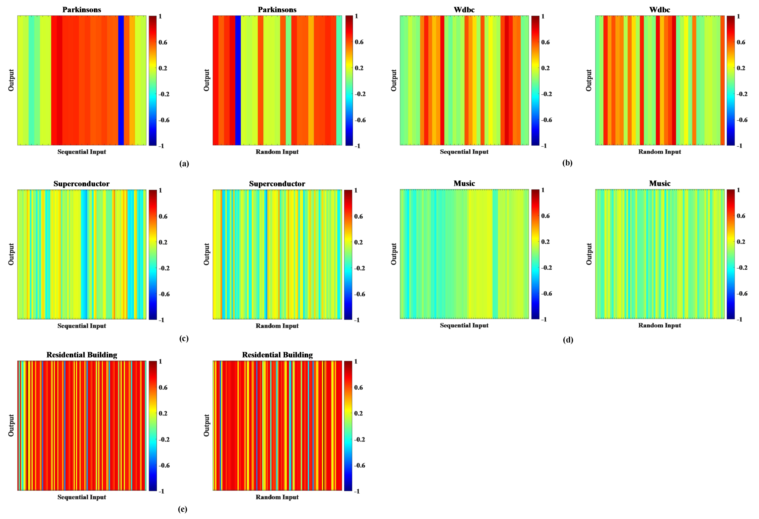
The analysis of the effect of different combinations of submodule inputs: By analyzing the structure of the DNFS, the combination of inputs for each submodule of the first layer played a key role in improving the performance of the DNFS. Therefore, we performed the Pearson correlation analysis on the confusion inputs of the first layer obtained in the experiments with the output variable. Figure 5 shows the correlation analysis diagram between the output and inputs sequentially and randomly on the five datasets. It can be seen obviously that the input variables with high correlation values were relatively concentrated both sequentially and in the random cases on Dataset No. 1 and No. 3. On the contrary, the inputs with high correlation values were more scattered in the random case than that of the sequential case on Dataset No.2, No. 4, and No. 5.

Meanwhile, the results of

Table 8. The performance of different algorithms on Test Dataset No. 1.

Methods	AIC	MAE	RMSE	SMAPE	Score	No. of Params	Time (s)
DNFS5-2	−10,960.29	0.036194	0.048819	3.6826%	22	1616	79.17
DNFS5-2-Random	−10,586.60	0.038558	0.052859	3.8531%	18	1616	79.17
MBGD-RDA	−11,543.80	0.060311	0.078368	5.8256%	12	212	80.60
RBF	−11,197.62	0.056373	0.075138	5.6249%	14	484	4.45
GRNN	151,331.14	0.076540	0.100070	7.3024%	4	81,075	0.75
LSTM	−5155.65	0.053984	0.071124	5.3900%	14	3634	11.27

,

Table 9. The performance of different algorithms on Test Dataset No. 2.

Methods	AIC	MAE	RMSE	SMAPE	Score	No. of Params	Time (s)
DNFS5-2	97.92	0.034611	0.045798	5.4495%	19	752	3.24
DNFS5-2-Random	−49.68	0.021180	0.033134	3.3494%	23	752	3.24
MBGD-RDA	−876.94	0.044928	0.057675	7.1593%	14	212	11.55
RBF	744.59	0.046341	0.075619	7.0748%	10	961	2.85
GRNN	20,721.73	0.065567	0.089166	9.5434%	4	10,912	0.23
LSTM	13,319.86	0.036128	0.048267	5.9079%	14	7351	3.69

,

Table 10. The performance of different algorithms on Test Dataset No. 3.

Methods	AIC	MAE	RMSE	SMAPE	Score	No. of Params	Time (s)
DNFS5-2	−12,060.34	0.072505	0.096758	7.4269%	19	3312	136.01
DNFS5-2-Random	−12,267.30	0.070064	0.094287	7.2362%	23	3312	136.01
MBGD-RDA	−15,879.33	0.107280	0.130300	10.2332%	15	212	133.09
RBF	−4768.90	0.079133	0.102580	8.1977%	15	6724	55.13
GRNN	980,721.60	0.128060	0.148110	11.6646%	4	498,000	4.66
LSTM	89,774.67	0.111550	0.135110	10.6297%	8	52,894	61.63

,

Table 11. The performance of different algorithms on Test Dataset No. 4.

Methods	AIC	MAE	RMSE	SMAPE	Score	No. of Params	Time (s)
DNFS5-2	4360.27	0.14319	0.19193	7.4534%	17	2880	18.98
DNFS5-2-Random	4205.55	0.11462	0.15992	6.0446%	23	2880	18.98
MBGD-RDA	−962.79	0.15571	0.19488	8.1886%	11	212	17.95
RBF	8462.11	0.15690	0.20645	8.0534%	7	4900	3.04
GRNN	88,733.52	0.14374	0.18379	7.4592%	14	45,085	0.27
LSTM	75,437.50	0.14707	0.18509	7.6936%	12	38,434	7.72

and

Table 12. The performance of different algorithms on Test Dataset No. 5.

Methods	AIC	MAE	RMSE	SMAPE	Score	No. of Params	Time (s)
DNFS5-2	16,098.64	0.054051	0.095032	9.0792%	14	8400	27.58
DNFS5-2-Random	15,720.91	0.014918	0.026753	3.8346%	23	8400	27.58
MBGD-RDA	−274.07	0.065187	0.096086	9.4366%	12	212	8.79
RBF	23,125.08	0.070965	0.117970	11.0976%	6	11,881	3.08
GRNN	48,221.88	0.044081	0.060055	7.4286%	17	24,530	0.24
LSTM	186,906.80	0.055241	0.068434	8.9043%	12	93,853	6.80

indicate that DNFS5-2-Random achieved better performance than DNFS5-2 on Dataset No. 2, No. 4, and No. 5. Compared with DNFS5- 2, DNFS5-2-Random decreased by 38.8%, 27.7%, and 38.5% the MAE, RMSE, and SMAPE for Test Dataset No. 2, while it decreased them by 19.9%, 16.7%, and 18.9% for Test Dataset No. 4, and by 72.4%, 71.8%, and 57.7% for Test Dataset No. 5, respectively. However, their performance was not significantly differences on the other two datasets.

Through the analysis of the results obtained, it can be concluded that the features that had a higher correlation with the output should be dispersed into each submodule, so that the performance of each submodule can be balanced and the overall performance improved.

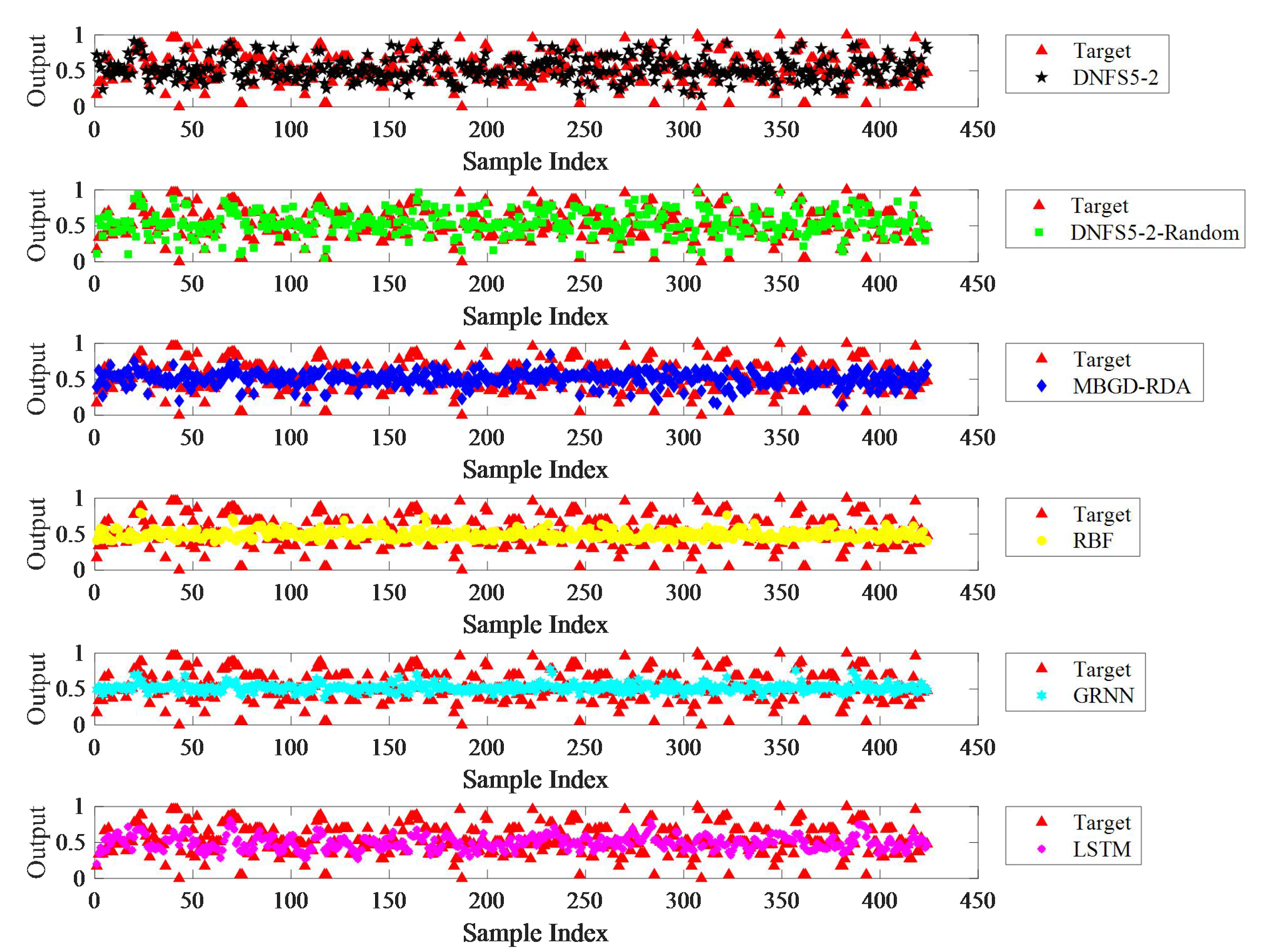
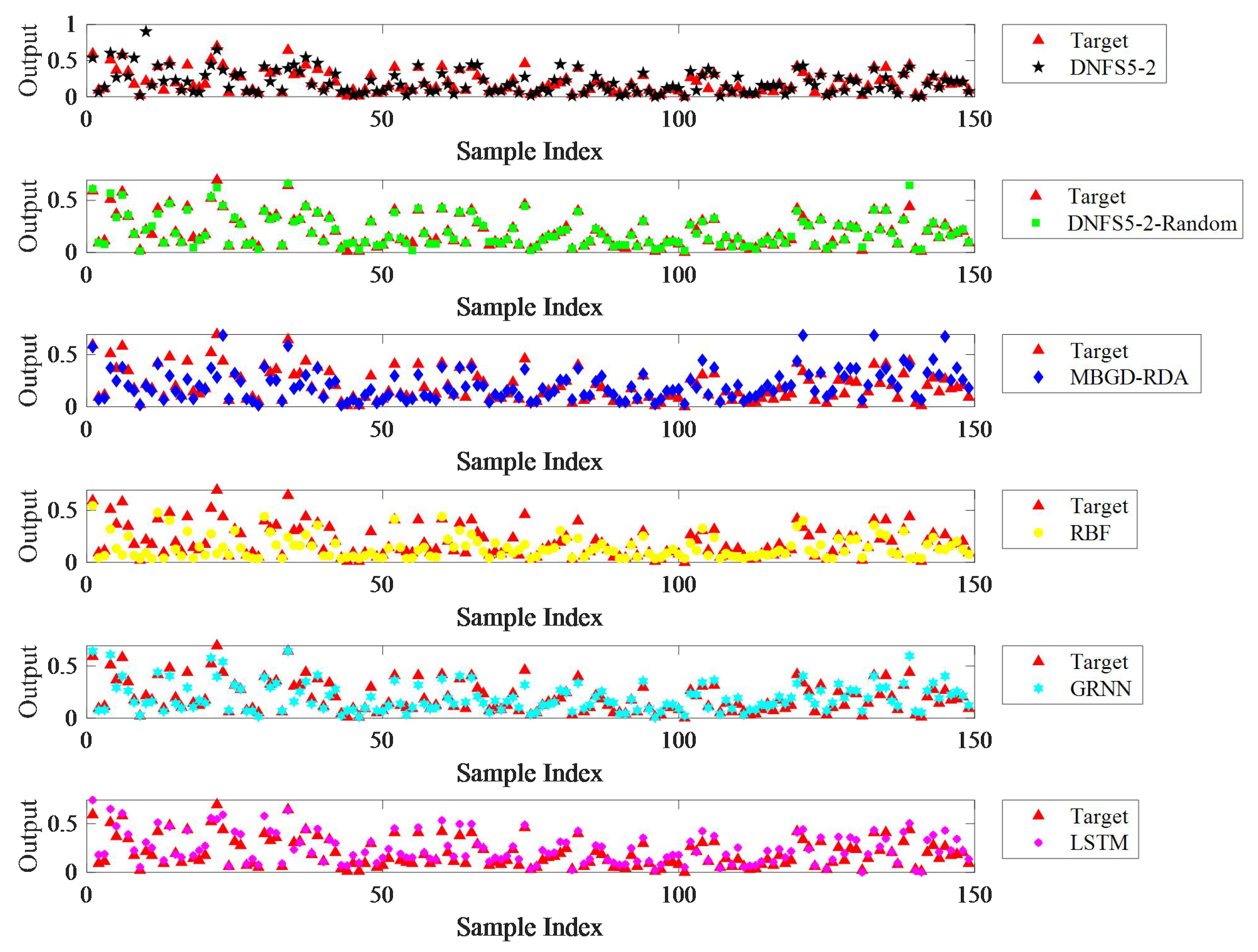
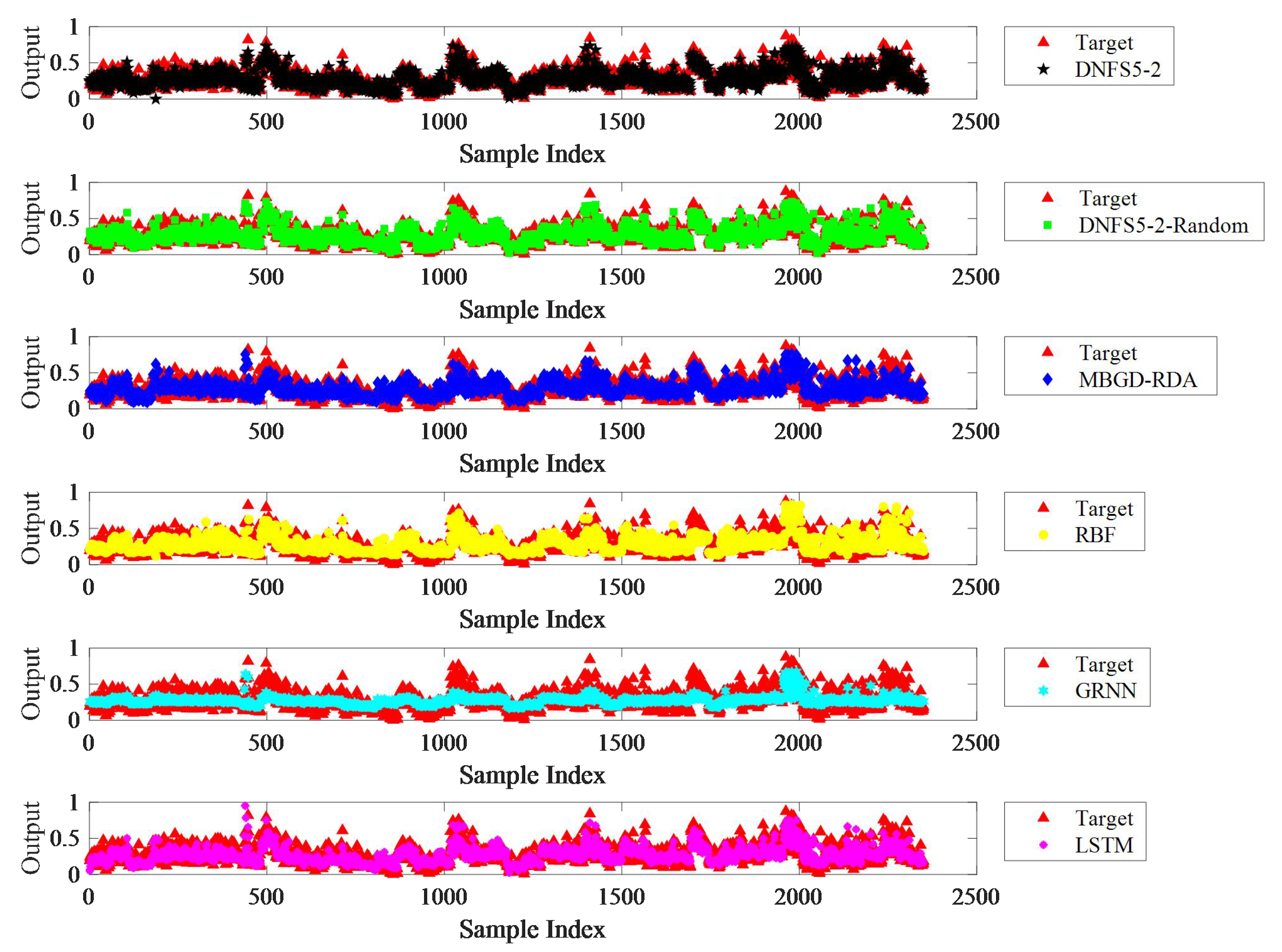
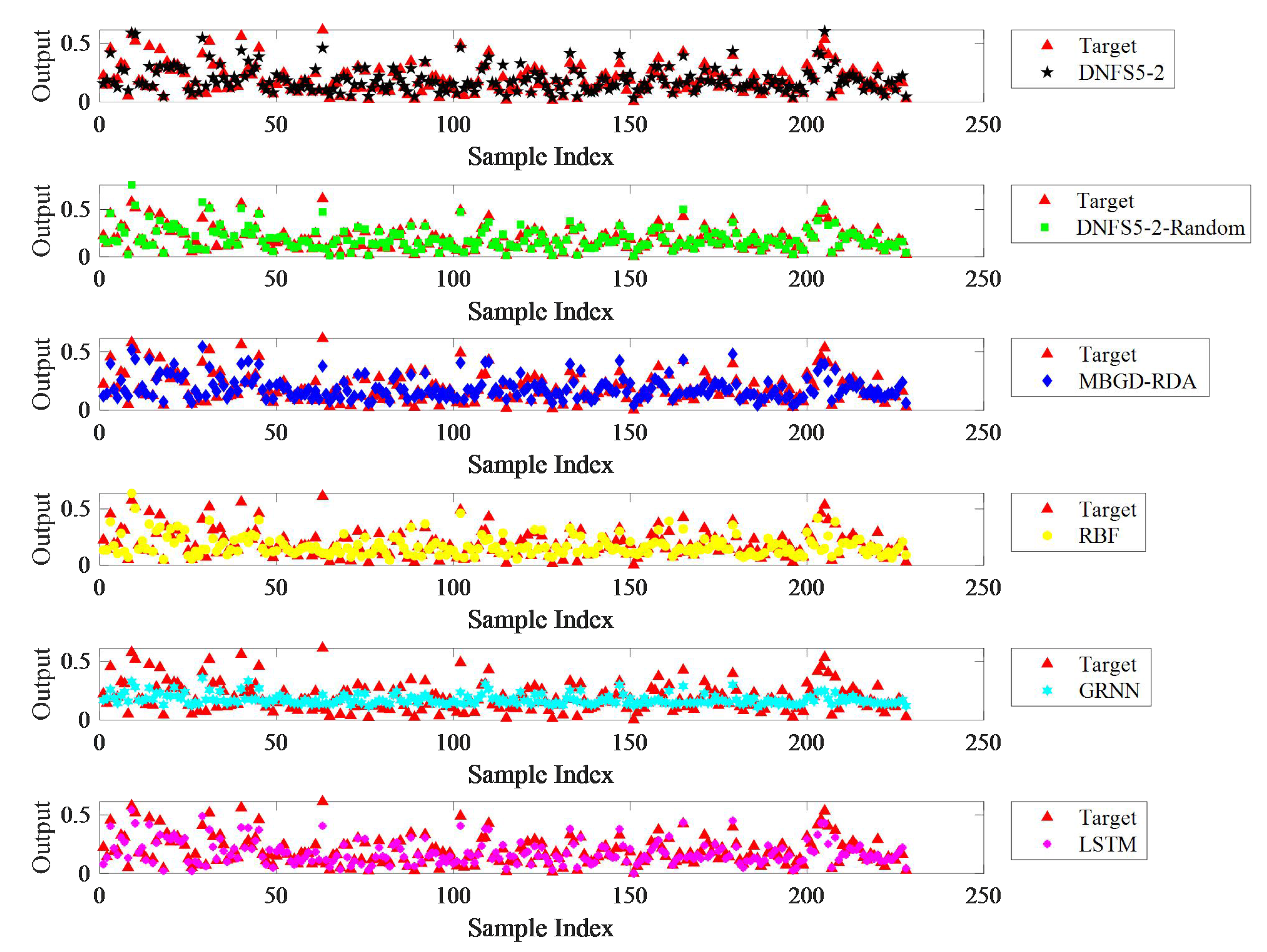
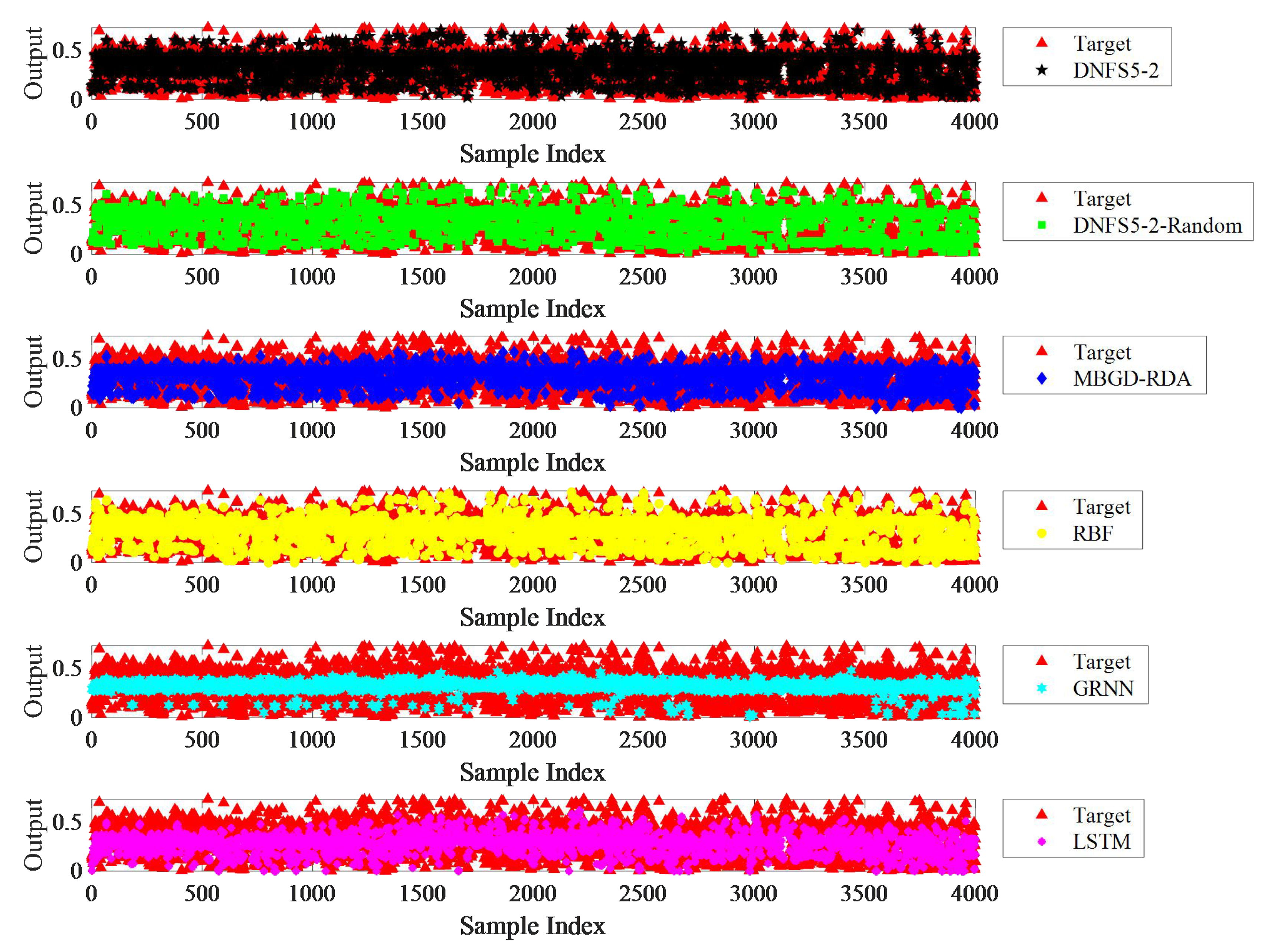
The analysis of the performances of the DNFS and the other algorithms: The performance comparison of the DNFS with the other algorithms on the five test datasets is shown in Table 8, Table 9, Table 10, Table 11 and Table 12. The prediction charts for different algorithms are shown in Figure 6, Figure 7, Figure 8, Figure 9 and Figure 10. Through observation and analysis, the following information can be obtained:

As shown in Figure 6, Figure 7, Figure 8, Figure 9 and Figure 10, DNFS5-2-Random achieved the highest prediction accuracy among the six algorithms on the five datasets. Compared to MBGD-RDA, RBF, GRNN, and LSTM, the average MAE decreased by 40.1%, 36.7%, 43.3%, and 35.8%, respectively, the average RMSE decreased by 34.1%, 36.4%, 36.8%, and 27.7%, respectively, and the average SMAPE decreased by 40.4%, 39.2%, 43.9%, and 36.8% respectively. The performance of DNFS5-2 was second only to DNFS5-2-Random. Compared to MBGD-RDA, RBF, GRNN, and LSTM, the average MAE of DNFS5-2 was reduced by 21.4%, 16.8%, 25.6%, and 15.6%, respectively, the average RMSE decreased by 14.1%, 17.2%, 17.6%, and 5.8%, respectively, and the average SMAPE decreased by 18.9%, 17.3%, 23.7%, and 14.1%, respectively. Hence, there is no doubt that the DNFS outperformed the other algorithms in prediction accuracy.

Meanwhile, Table 8, Table 9, Table 10, Table 11 and Table 12 show that DNFS5-2 had fewer parameters and a simpler structure than RBF, GRNN, and LSTM, which validated that DNFS5-2 has less complexity and higher interpretability. On the contrary, the parameters of the three machine learning models increased exponentially with the dimensionality of the input, which led to their interpretability being very poor. In addition, MBGD-RDA constrained the maximum input dimensionality five, so that its parameters were equal to 212 (5 ∗ 2 ∗ 2 + $2^5$ ∗ (5 + 1) = 212), while the MF was Gaussian and the number for each input domain was two. On all five datasets, the parameters of MBGD-RDA were far fewer than the other algorithms, resulting in the AIC being minimum. However, the prediction accuracy of MBGD-RDA was not optimal, which was probably because of the loss of important features due to PCA, so the performance was greatly affected.

The average computational time that DNFS5-2, MBGD-RDA, RBF, GRNN, and LSTM spent on the five datasets was 52.99 s, 50.39 s, 13.31 s, 1.23 s, and 18.22 s respectively. Obviously, GRNN was the most efficient method among all the algorithms. Although the efficiency of DNFS5-2 was relatively poor, it could achieve the best performance within a valid period of time, which could not be achieved by previous FSs. Additionally, the computational cost for each algorithm increased with the features and samples based on Table 8, Table 9, Table 10, Table 11 and Table 12.

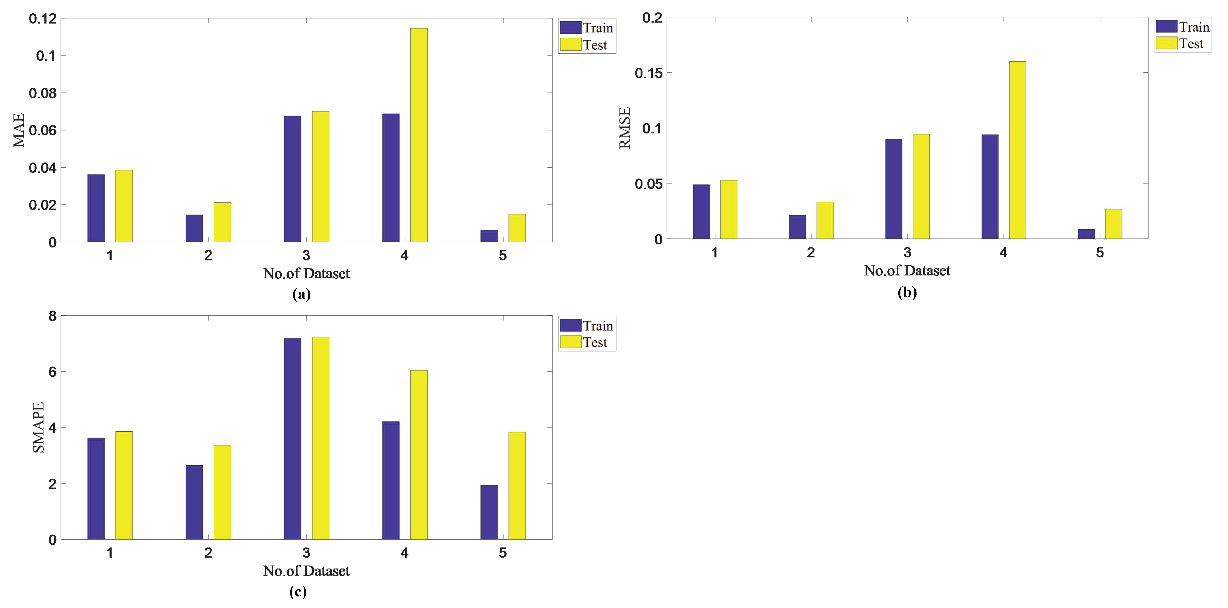
The analysis of the generalization ability of the DNFS: The performance comparison of the DNFS on the five datasets for the training and the testing is shown in Figure 11. Figure 11a shows the test MAE comparison of the DNFS on the training level with the testing level, while Figure 11b,c shows the test RMSE and SMAPE comparison, respectively. It can be seen that the DNFS could achieve excellent performance both on the training level and testing level. The DNFS had similar performance on the training level and testing level, in particular for Dataset No. 1 and No. 3. It is obvious that the DNFS had excellent generalization performance with enough samples. However, the test performance would be slightly worse than that on the training level due to fewer samples. Therefore, the regularization method will be introduced in the future research to enhance the generalization ability of the DNFS.

5. Conclusions

FSs are well-known machine learning models, but have difficulty in dealing with high-dimensional data. This paper proposed the DNFS to enable FSs to effectively solve high-dimensional regression problems on the basis of ensuring accuracy and interpretability. Inspired by deep learning, the SC-ANFIS was proposed and adopted as a submodule to construct the structure of the DNFS in a bottom-up way. This paper also performed an in-depth study on the deep structure and the combination of submodule inputs for the DNFS to improve the performance of the DNFS.

The experimental results on five real-world regression datasets indicated that:

• The DNFS had higher prediction accuracy. Compared with the well-known models: MBGD-RDA, RBF, GRNN, and LSTM, the average values of the DNFS on MAE, RMSE, and SMAPE decreased by 38.9%, 33.7%, and 40.0%, respectively;
• The DNFS had less complexity and better interpretability. The number of parameters of the DNFS was far less than the other algorithms, especially when the dimensionality of the input was very high. It also can be concluded that the structure of the DNFS is simpler and more interpretable;
• The DNFS can solve high-dimensional regression problems in a more reasonable time than the previous FSs, while ensuring excellent performance;
• The DNFS with five submodule inputs and two shared inputs had the best comprehensive performance. Additionally, dispersing the features that had a high correlation with the output into each submodule, better improvement of the DNFS could be achieved.

Additionally, this paper proposes future research directions: On the one hand, how to reduce the time consumption under the same structure will be further considered. Removing the submodules with poor performance or more fuzzy rules is the current preliminary idea, which is likely to reduce the computational cost and improve the accuracy. On the other hand, how to determine the optimal input combination for each submodule is also another future direction.

References

1. Zadeh, L.A. Fuzzy sets. Inf. Control. 1965, 8, 338–353. [Google Scholar] [CrossRef] [Green Version]
2. Li, J.S.; Gong, Z.T. SISO intuitionistic fuzzy systems: IF-t-norm, IF-R-implication and universal approximators. IEEE Access 2019, 7, 70265–70278. [Google Scholar] [CrossRef]
3. Harirchian, E.; Lahmer, T. Improved Rapid Assessment of Earthquake Hazard Safety of Structures via Artificial Neural Networks. IOP Conf. Ser. Mater. Sci. Eng. 2020, 897, 012014. [Google Scholar] [CrossRef]
4. Harirchian, E.; Jadhav, K.; Kumari, V.; Lahmer, T. ML-EHSAPP: A prototype for machine learning-based earthquake hazard safety assessment of structures by using a smartphone app. Eur. J. Environ. Civ. Eng. 2021, 3, 1–21. [Google Scholar] [CrossRef]
5. Harirchian, E.; Hosseini, S.E.A.; Jadhav, K.; Kumari, V.; Rasulzade, S.; Işık, E.; Wasif, M.; Lahmer, T. A review on application of soft computing techniques for the rapid visual safety evaluation and damage classification of existing buildings. J. Build. Eng. 2021, 43, 102536. [Google Scholar] [CrossRef]
6. Mattar, M.A.; El-Marazky, M.S.; Ahmed, K.A. Modeling sprinkler irrigation infiltration based on a fuzzy-logic approach. Span. J. Agric. Res. 2017, 15, 1–10. [Google Scholar] [CrossRef] [Green Version]
7. Fan, T.; Xu, J. Image Classification of Crop Diseases and Pests Based on Deep Learning and Fuzzy System. Int. J. Data Warehous. Min. 2020, 16, 34–47. [Google Scholar] [CrossRef]
8. Cui, Y.Q.; Wu, D.R.; Huang, J. Optimize TSK Fuzzy Systems for Classification Problems: Minibatch Gradient Descent With Uniform Regularization and Batch Normalization. IEEE Trans. Fuzzy Syst. 2020, 28, 3065–3075. [Google Scholar] [CrossRef] [Green Version]
9. Wu, D.R.; Tang, X. Multitasking Genetic Algorithm (MTGA) for Fuzzy System Optimization. IEEE Trans. FS. 2020, 28, 1050–1061. [Google Scholar] [CrossRef] [Green Version]
10. Bisht, D.; Jain, S.; Srivastava, P.K. Adaptive Particle Swarm Optimized Fuzzy Algorithm to Predict Water Table Elevation. Int. J. Model. Simul. Sci. Comput. 2019, 10, 1950038. [Google Scholar] [CrossRef]
11. Jafari, R.; Razvarz, S.; Gegov, A. A Novel Technique for Solving Fully Fuzzy Nonlinear Systems Based on Neural Networks. Vietnam. J. Comput. Sci. 2020, 7, 93–107. [Google Scholar] [CrossRef] [Green Version]
12. Jang, J.S.R. ANFIS: Adaptive-network-based fuzzy inference system. IEEE Trans. Syst. Man Cybern. 1993, 23, 665–685. [Google Scholar] [CrossRef]
13. Barak, S.; Sadegh, S.S. Forecasting energy consumption using ensemble ARIMA-ANFIS hybrid algorithm. Int. J. Electr. Power Energy Syst. 2016, 82, 92–104. [Google Scholar] [CrossRef] [Green Version]
14. Panapakidis, I.P.; Dagoumas, A.S. Day-ahead natural gas demand forecasting based on the combination of wavelet transform and ANFIS/genetic algorithm/neural network model. Energy 2017, 118, 231–245. [Google Scholar] [CrossRef]
15. Dieu, T.B.; Khabat, K.; Shaojun, L.; Himan, S.; Mahdi, P.; Vijay, P.S.; Kamran, C.; Ataollah, S.; Somayeh, P.; Wei, C.; et al. New Hybrids of ANFIS with Several Optimization Algorithms for Flood Susceptibility Modeling. Water 2018, 10, 1210. [Google Scholar]
16. Kisi, O.; Demir, V.; Kim, S. Estimation of long-term monthly temperatures by three different adaptive neuro-fuzzy approaches using geographical inputs. J. Irrig. Drain. Eng. 2017, 143, 04017052. [Google Scholar] [CrossRef]
17. Begic, F.L.; Avdagic, A.; Besic, I. Prediction of Heart Attack Risk Using GA-ANFIS Expert System Prototype. Stud. Health Technol. Inform. 2015, 211, 292. [Google Scholar]
18. Naa, A.; Sgm, B.; Zk, C. The prediction of longitudinal dispersion coefficient in natural streams using LS-SVM and ANFIS optimized by Harris hawk optimization algorithm. J. Contam. Hydrol. 2021, 240, 103781. [Google Scholar]
19. Xu, L.; Huang, C.; Li, C.; Wang, J. Estimation of tool wear and optimization of cutting parameters based on novel ANFIS-PSO method toward intelligent machining. J. Intell. Manuf. 2021, 32, 1–4. [Google Scholar] [CrossRef]
20. Kaur, S.; Chahal, K.K. Hybrid ANFIS-genetic algorithm based forecasting model for predicting Cholera-waterborne disease. Int. J. Intell. Eng. Inform. 2020, 8, 374. [Google Scholar]
21. Balasubramanian, K.; Ananthamoorthy, N.P. Improved adaptive neuro-fuzzy inference system based on modified glowworm swarm and differential evolution optimization algorithm for medical diagnosis. Neural Comput. Appl. 2021, 33, 1–12. [Google Scholar] [CrossRef]
22. Mohammad, A.; Fang, Y.T.; Ali, N.A.; Sarmad, D.L.; Yuk, F.H.; Osama, A.; Nadhir, A.A.; Ahmed, E.S. Performance improvement for infiltration rate prediction using hybridized Adaptive Neuro-Fuzzy Inferences System (ANFIS) with optimization algorithms. Ain Shams Eng. J. 2021, 12, 1665–1676. [Google Scholar]
23. Beattie, J.R. Esmonde-White, FWL, Exploration of Principal Component Analysis: Deriving Principal Component Analysis Visually Using Spectra. Appl. Spectrosc. 2021, 75, 361–375. [Google Scholar] [CrossRef]
24. Razin, M.; Voosoghi, B. Ionosphere time series modeling using adaptive neuro-fuzzy inference system and principal component analysis. GPS Solut. 2020, 24, 1–13. [Google Scholar]
25. Hcp, A.; Htd, B. Predicting burst pressure of defected pipeline with Principal Component Analysis and Adaptive Neuro Fuzzy Inference System. Int. J. Press. Vessel. Pip. 2021, 189, 104274. [Google Scholar]
26. Wu, D.R.; Yuan, Y.; Huang, J.; Tan, Y. Optimize TSK FS for Regression Problems: Minibatch Gradient Descent With Regularization, DropRule, and AdaBound (MBGD-RDA). IEEE Trans. Fuzzy Syst. 2020, 28, 1003–1015. [Google Scholar] [CrossRef] [Green Version]
27. Karaboga, D.; Kaya, E. Adaptive network based fuzzy inference system (ANFIS) training approaches: A comprehensive survey. Artif. Intell. Rev. 2019, 52, 2263–2293. [Google Scholar] [CrossRef]
28. Abdolkarimi, E.S.; Mosavi, M.R. Wavelet-adaptive neural subtractive clustering fuzzy inference system to enhance low-cost and high-speed INS/GPS navigation system. GPS Solut. 2020, 24, 1–17. [Google Scholar] [CrossRef]
29. Mola, M.; Amiri-Ahouee, R. ANFIS model based on fuzzy C-mean, grid partitioning and subtractive clustering to detection of stator winding inter-turn fault for PM synchronous motor. Int. Trans. Electr. Energy Syst. 2021, 31, e12770. [Google Scholar] [CrossRef]
30. Tiwari, S.; Babbar, R.; Kaur, G. Performance Evaluation of Two ANFIS Models for Predicting Water Quality Index of River Satluj (India). Adv. Civ. Eng. 2018, 3, 1–10. [Google Scholar] [CrossRef] [Green Version]
31. Moradi, F.; Bonakdari, H.; Kisi, O.; Ebtehaj, I.; Shiri, J.; Gharabaghi, B. Abutment scour depth modeling using neuro-fuzzy-embedded techniques. Mar. Georesources Geotechnol. 2019, 37, 190–200. [Google Scholar] [CrossRef]
32. Safari, M.; Ebtehaj, I.; Bonakdari, H.; Es-haghi, M. Sediment transport modeling in rigid boundary open channels using generalize structure of group method of data handling. J. Hydrol. 2019, 577, 123951. [Google Scholar] [CrossRef]
33. Yaseen, Z.M.; Ebtehaj, I.; Bonakdari, H.; Deo, R.C.; Mehr, A.D.; Mohtar, W.H.; Diop, L.; El-Shafie, A.; Singh, V.P. Novel approach for streamflow forecasting using a hybrid ANFIS-FFA model. J. Hydrol. 2017, 554, 263–276. [Google Scholar] [CrossRef]
34. Yilmaz, M.; Arslan, E. Effect of the Type of Membership Function on Geoid Height Modelling with Fuzzy Logic. Surv. Rev. 2008, 40, 379–391. [Google Scholar] [CrossRef]
35. Sambariya, D.K.; Prasad, R. Selection of Membership Functions Based on Fuzzy Rules to Design an Efficient Power System Stabilizer. Int. J. Fuzzy Syst. 2017, 19, 813–828. [Google Scholar] [CrossRef]
36. Bonakdari, H.; Moeeni, H.; Ebtehaj, I.; Zeynoddin, M.; Mahoammadian, A.; Gharabaghi, B. New insights into soil temperature time series modeling: Linear or nonlinear. Theor. Appl. Climatol. 2019, 135, 1157–1177. [Google Scholar] [CrossRef]
37. Gholami, A.; Bonakdari, H.; Ebtehaj, I.; Shaghaghi, S.; Khoshbin, F. Developing an expert group method of data handling system for predicting the geometry of a stable channel with a gravel bed. Earth Surf. Process. Landf. 2017, 42, 1460–1471. [Google Scholar] [CrossRef]
38. Chen, X.; Yang, W.Q. Prediction and Analysis of Literature Loan Circulation in University Libraries Based on RBF Neural Network Optimized Model. Autom. Control. Comput. Sci. 2020, 54, 139–146. [Google Scholar] [CrossRef]
39. Li, A.; Yang, X.; Xie, Z.; Yang, C. An optimized GRNN-enabled approach for power transformer fault diagnosis. IEEJ Trans. Electr. Electron. Eng. 2019, 14, 1181–1188. [Google Scholar] [CrossRef]
40. Comesaa, M.M.; Febrero-Garrido, L.; Troncoso-Pastoriza, F.; Martínez-Torres, J. Prediction of building’s thermal performance using lstm and mlp neural networks. Appl. Sci. 2020, 10, 7439. [Google Scholar]
Figure 1. The general structure diagram of DNFS5-2.
Applsci 11 07766 g001
Figure 2. The flowchart of DNFSm-n.
Applsci 11 07766 g002
Figure 3. Prediction chart of DNFSs with different submodule inputs on the three test datasets. (a) Test Dataset No. 1. (b) Test Dataset No. 2. (c) Test Dataset No. 3.
Applsci 11 07766 g003
Figure 4. Prediction chart of DNFSs with different shared inputs on the three test datasets. (a) Test Dataset No. 1. (b) Test Dataset No. 2. (c) Test Dataset No. 3.
Applsci 11 07766 g004
Figure 5. Correlation analysis comparison of sequential inputs with random inputs. (a) The random inputs were obtained from Dataset No. 1. (b) The random inputs were obtained from Dataset No. 2. (c) The random inputs were obtained from Dataset No. 3. (d) The random inputs were obtained from Dataset No. 4. (e) The random inputs were obtained from Dataset No. 5.
Applsci 11 07766 g005
Figure 6. Prediction charts of different algorithms on Test Dataset No. 1.
Applsci 11 07766 g006
Figure 7. Prediction charts of different algorithms on Test Dataset No. 2.
Applsci 11 07766 g007
Figure 8. Prediction charts of different algorithms on Test Dataset No. 3.
Applsci 11 07766 g008
Figure 9. Prediction charts of different algorithms on Test Dataset No. 4.
Applsci 11 07766 g009
Figure 10. Prediction charts of different algorithms on Test Dataset No. 5.
Applsci 11 07766 g010
Figure 11. Performance of the DNFS on the five datasets for the training and testing. (a) The test MAE comparison. (b) The test RMSE comparison. (c) The test SMAPE comparison.
Applsci 11 07766 g011