Nonlinear Loads Compensation Using a Shunt Active Power Filter Controlled by Feedforward Neural Networks

Abstract

The shunt active power filter (SAPF) is a widely used tool for compensation of disturbances in three-phase electric power systems. A high number of control methods have been successfully developed, including strategies based on artificial neural networks. However, the typical feedforward neural network, the multilayer perceptron, which has provided effective solutions to many nonlinear problems, has not yet been employed with satisfactory performance in the implementation of the SAPF control for obtaining the reference currents. In order to prove the capabilities of this simple neural topology, this work describes a suitable strategy of use, based on the accurate estimation of the Fourier coefficients corresponding to the fundamental harmonic of any distorted voltage or current. An effective training method has been developed, consisting of the use of many distorted patterns. The new generation procedure uses random combinations of multiple harmonics, including the possible nominal frequency deviations occurring in real power systems. The design of the generation of reference signals through computations based on the Fourier coefficients is presented. The objectives were the harmonic mitigation and power factor correction. Practical cases were tested through simulation and also by using an experimental platform, showing the feasibility of the proposal.

1. Introduction

The increase in disturbances in the electric power distribution networks due to the presence of harmonics has given rise to an exhaustive search for solutions in the past three decades. The compensation objectives to enhance the electric power quality (EPQ) may be varied, including issues such as reactive power compensation, reduction in harmonic distortion, or correction of unbalanced three-phase currents. Therefore, different active and passive filter configurations have been proposed to solve these problems. Among them, the most important tool for improving the EPQ is the active power filter (APF), and in particular, the shunt APF. This compensation system is more and more relevant, thanks to the development of signal processing and power converters [1,2].

The shunt APF consists of an electronic power converter for use in three-phase systems, connected in parallel with the load to supply compensation currents. The converter is typically based on insulated gate bipolar transistors (IGBTs) and the pulse width modulation technique (PWM), and provides the currents that mitigate the EPQ problems. A control system must generate the appropriate trigger pulses to switch the on-off states of the electronic power devices of the converter, in order to achieve the right output currents. Previously, depending on the compensation goal, the appropriate reference signals for those currents had to be generated. This means that two essential elements in the APF control are the generation of the reference signals and the PWM control method, such as hysteresis band control (HB) [2]. Other important issues are the control of the power converter DC side [3] and the phase synchronization techniques [4]. The purpose of some APF control methods is limited to harmonic distortion mitigation, whereas many others try to achieve both harmonic suppression and reactive power compensation and may include addressing the load currents unbalance.

The use of artificial neural networks (ANN) in the field of power engineering is well known. They make use of parallel computing, allowing the design of control circuits of high speed and reliability. In fact, ANNs have been systematically applied in the development of APF-based equipment, even though there are countless examples of non-ANN control techniques, as in [5,6,7]. A type of ANN usually applied to the APF control is the Adaline, based on the adaptive algorithm of Widrow–Hoff. Thus, in [8,9], the Adaline network is used for extraction of the reference currents and the multilayer perceptron network (MLP) replaces the HB control. Moreover, in [10,11,12,13], the core of the APF control is an Adaline network, which works with an on-line algorithm, under different load conditions. The work in [14] shows a comparative review of several control methods, including the study of the Adaline, highlighting some of its advantages. However, in these adaptive cases, the appropriate choice of the learning parameter for each problem is very important in order to avoid convergence problems; this is one of its weaknesses. However, recent works [15,16,17] illustrate that researchers continue to propose advances in the application of the Adaline. Other ANN types have also been applied to the APF, but with less relevance. This is the case of the radial basis function networks (RBF) and different topologies of recurrent neural networks (RNN). The RBF has been applied in [18] for extracting harmonic amplitudes, in [19] to support a complex adaptive sliding mode control (SMC), and in [20], it is used in combination with the P-Q power theory to obtain reference signals. Regarding the RNN, which has a structure close to the MLP, but with internal feedback connections, in [21,22], it supports complex types of sliding mode controls in the APF. The authors of [23] achieved good results using the so-called NARX recurrent network for extracting the reference signals. Additionally, the RNN called echo-state network (ESN) has gained importance in recent years for extracting fundamental current components [24,25].

The feedforward or MLP networks have shown to be useful in replacing the HB controller to generate the IGBTs trigger signals [8,9,17,26,27]. Some authors have applied the MLP [28,29,30] to replace the extended PI control [31] of the DC side capacitor voltage, Vdc, of power converters. To a lesser extent, the MLP networks have also been used to obtain the reference signals [32,33], with variable results. MLP networks seemed to be a promising tool for harmonic detection and mitigation many years ago [32,34,35,36]. Nevertheless, they could not be successfully applied for the generation of the reference currents when trying to achieve accurate APF control for all kinds of distortions. They are not adaptive, requiring a previous off-line training using the backpropagation algorithm (BP). Some researchers directly claim limitations of the MLP by generating the reference signals, due to the diversity of loads and kinds of electric disturbances [24,33]. Even the works which conclude supporting the capabilities of this ANN type show poor results [32] and weaknesses—it is difficult to apply a training capable of covering high order harmonics, as well as the possible practical frequency deviations.

It is also worth mentioning the numerous methods combining fuzzy logic and ANNs in different ways. As an example, in [37], a combination of fuzzy and neural network techniques is used for improved DC voltage control by an APF, where a fuzzy logic controller extracts the training dataset for the neural network. In [38], an adaptive backstepping fuzzy neural network controller is designed to suppress the harmonics in a SAPF.

In this paper, the main features are as follows. Firstly, a new MLP-based control method for three-phase shunt APFs, able to obtain the reference signals, is proposed. It will prove that this ANN type can provide an alternative tool, which will allow taking advantage of the benefits of MLPs, such as simplicity, no need of online training, fast response, and the absence of internal feedback connections within the network. Secondly, the strategy of use of the ANN consists of estimating the Fourier coefficients of the fundamental harmonic of phase currents and voltages, enabling higher MLP learning capacity than different methods tested by the authors. Thirdly, an effective training method was designed, in which the waveform patterns are automatically generated using random combinations of many different harmonics. Variable fundamental frequencies were included in the patterns, representing the possible nominal frequency deviations in the grid, ensuring a robust control response in different real cases. This method has shown to be more efficient for the MLP learning than any other previously applied. It provides a deep training with a high, but limited, number of patterns. Fourthly, for a compensation strategy that pursues harmonic distortion mitigation and power factor correction, the power theory was applied to develop the computation steps, from the coefficients of every phase current and voltage that lead to the reference currents. The method also will be able to correct the currents’ unbalance, in the case of balanced supply voltages. The paper is structured as follows. In Section 2, the fundamentals of the control strategies are described. Section 3 addresses the explanation of the neural network configuration and the training steps carried out. In Section 4, practical cases are simulated and thoroughly tested using the MATLAB-Simulink platform, and a practical case is tested in laboratory. Finally, the conclusions highlight the contributions of the work.

2. Principles of the Compensation Methods

Figure 1 shows the scheme of a nonlinear three-phase load compensated by a shunt APF. The currents generated by the APF must be such that they satisfy the compensation requirements and verify Kirchhoff’s currents law.

$$i_S=i_L-i_C$$

(1)

Two main compensation objectives are considered: harmonic compensation (HC) and unit power factor compensation (UpfC). The HC pursues a source current without distortion. The UpfC aims to obtain a source current in phase with the voltage, in addition to harmonic compensation. The foundations of both techniques are established in the following subsections.

2.1. Harmonic Compensation Method

The first compensation objective considered here is the mitigation of the harmonic distortion of the load current. It is well known that the waveform of a distorted current can be represented by the sum of different sinusoidal components with frequencies that are a multiple of a fundamental frequency. Equation (2) shows the expression for a generic phase current of a nonlinear load.

$$i_{L,i}(t)=\sqrt{2}\hspace{0.17em}{I}_{1,i}\hspace{0.17em}\cos \left(\omega \hspace{0.17em}t-{\phi }_{1,i}\right)+\sqrt{2}\hspace{0.17em}{\displaystyle \sum _{\forall \hspace{0.17em}h\ge 2}{I}_{h,i}\hspace{0.17em}\cos \left(h\hspace{0.17em}\omega \hspace{0.17em}t-{\phi }_{h,i}\right)}$$

(2)

$$i_{c,i}(t)=i_{L,i}(t)-i_{s,i}(t)=\sqrt{2}\hspace{0.17em}{\displaystyle \sum _{\forall \hspace{0.17em}\hspace{0.17em}h\ge 2}{I}_{h,i}\hspace{0.17em}\cos \left(h\hspace{0.17em}\omega \hspace{0.17em}t-{\phi }_{h,i}\right)}$$

(3)

Equation (3) consists of all the distortion components of the load current. The compensation current (3) allows obtaining a set of sinusoidal currents; thus, after compensation, the source currents are given by (4):

$$i_{s,i}(t)=\hspace{0.17em}{i}_{L1,i}=\sqrt{2}\hspace{0.17em}{I}_{1,i}\hspace{0.17em}\cos \left(\omega \hspace{0.17em}t-{\phi }_{1,i}\right)$$

(4)

The currents (4) can be expressed through their rectangular components, (5):

$$\begin{array}{c}{i}_{s,\hspace{0.17em}i}(t)=\sqrt{2}\hspace{0.17em}{I}_{1,i}\hspace{0.17em}\cos \left(\omega \hspace{0.17em}t-{\phi }_{1,i}\right)=\sqrt{2}\hspace{0.17em}{I}_{1,i}\hspace{0.17em}\cos {\phi }_{1,i}\cos \omega \hspace{0.17em}t+\sqrt{2}\hspace{0.17em}{I}_{1,i}\hspace{0.17em}\sin {\phi }_{1,i}\sin \omega \hspace{0.17em}t=\\ A_{I,i}\cos \omega \hspace{0.17em}t+B_{I,i}\sin \omega \hspace{0.17em}t\end{array}$$

(5)

where A_I,i and B_I,i are real numbers that represent the rectangular coefficients of the fundamental harmonic of the phase current. It follows that the obtaining of each fundamental harmonic rectangular component of the phase currents determines the currents given by (5), and therefore, the compensation currents (3), which are finally expressed according to (6):

$$i_{c,i}(t)=i_{L,i}\left(t\right)-\left(A_{I,i}\cos \omega \hspace{0.17em}t+B_{I,i}\sin \omega \hspace{0.17em}t\right)$$

(6)

Three ANNs can estimate the pairs of rectangular coefficients, A_I,i, B_I,i. They constitute the core calculation of the reference currents for the APF control (Figure 2).

If a balanced three-phase system is assumed, the rectangular coefficients of the phase quantities are equal; in this case the second subscript i becomes unnecessary, with the coefficients becoming A_I, B_I. A single ANN would allow estimating the rectangular coefficients A_I, B_I, and hence the compensation currents (6), that can now be expressed according to (7):

$$\begin{array}{l}{i}_{c,a}(t)=i_{L,a}\left(t\right)-\left(A_I\cos \omega \hspace{0.17em}t+B_I\sin \omega \hspace{0.17em}t\right)\\ i_{c,b}(t)=i_{L,b}\left(t\right)-\left(A_I\cos (\omega \hspace{0.17em}t-2\pi /3)+B_I\sin (\omega \hspace{0.17em}t-2\pi /3)\right)\\ i_{c,c}(t)=i_{L,c}\left(t\right)-\left(A_I\cos (\omega \hspace{0.17em}t+2\pi /3)+B_I\sin (\omega \hspace{0.17em}t+2\pi /3)\right)\end{array}$$

(7)

Figure 2 shows the block diagram for the calculation of compensation currents; these are the reference signals in the APF control for HC. The sampling of the phase currents makes up the set of the neural network inputs. Its outputs are the rectangular coefficients that allow us to build the fundamental harmonic of each phase current. The subtraction with respect to the load currents provides the compensation currents. For a balanced nonlinear load, from (7) it follows that only a neural network is necessary, and therefore, it would only be necessary to sample a load current signal.

2.2. Unit Power Factor Compensation Method

In this second compensation method, the APF is required to inject the appropriate currents with the objectives of both mitigation of the harmonic distortion and achieving a unit power factor, measured from the source. The unit power factor objective will be achieved when the source current is in phase with the voltage, that is, when the source generates the so-called active current. In fact, it has been well established in the literature on electrical power that the active current is the current that carries the load active (average) power and is collinear with the source voltage. Hence, the phase currents of the source after compensation will take the form (8):

$$i_{s,i}(t)=G\hspace{0.17em}{v}_i\left(t\right)$$

(8)

where G is the so-called equivalent conductance parameter of the load defined by (9):

$$G=\frac{P_{}}{V_{}^2}=\frac{P_{}}{V_a^2+V_b^2+V_c^2}$$

(9)

In (9), P is the average power consumed by the load and V is the rms value of the three-phase voltage determined from the rms values of the phase voltages, V_i. Appendix A describes the way to obtain the value of G by knowing the voltage and current rectangular coefficients. In general, it requires six ANNs, according to Equation (A8): three ANNs for the six voltage rectangular coefficients, A_V,i, B_V,i, and three ANNs for the six rectangular coefficients of the current fundamental harmonic, A_I,i, B_I,i. It could be thought that perhaps it is a better strategy to train an ANN directly for estimation of G, instead of the coefficients, but in the authors’ experience, this strategy would require the use of a very high number of combinations of distorted waveforms of the six signals involved (three voltages and three currents), and would result in an excessive amount of data for the training algorithm.

If the source voltage is considered sinusoidal and balanced, then the different phase voltages are given by (10):

$$v_{s,i}(t)=\hspace{0.17em}\sqrt{2}\hspace{0.17em}{V}_i\hspace{0.17em}\cos \left(\omega \hspace{0.17em}t+{\alpha }_i\right)$$

(10)

where i = a, b, c. With Va = Vb = Vc, and αa = α, αb = α − 2π/3, αc = α + 2π/3. Thus, as in (4), the three phase voltages can be expressed according to (11):

$$\begin{array}{l}{v}_{s,a}(t)=A_V\cos \omega \hspace{0.17em}t+B_V\sin \omega \hspace{0.17em}t\\ v_{s,b}(t)=A_V\cos (\omega \hspace{0.17em}t-2\pi /3)+B_V\sin (\omega \hspace{0.17em}t-2\pi /3)\\ v_{s,c}(t)=A_V\cos (\omega \hspace{0.17em}t+2\pi /3)+B_V\sin (\omega \hspace{0.17em}t+2\pi /3)\end{array}$$

(11)

A single ANN can estimate the values of the voltage rectangular coefficients, A_V, B_V. In the same way, for currents, a single ANN can estimate the rectangular coefficients of the current fundamental harmonic, A_I, B_I, (7). Taking this into account, it follows that, in the case of balanced voltages and loads, only two ANNs are necessary and the expression in (A8) to obtain G would be as shown in (12):

$$G=\frac{A_V{A}_I+B_V{B}_I}{A_V^2+B_V^2}$$

(12)

The voltage and current rectangular coefficients can be estimated by the ANNs from the sampling of any of the phase quantities; that is why in (12), the double subscript i is no longer necessary.

The source currents after compensation can be identified with the active currents, (8), being the compensation currents injected by the APF given by (13):

$$i_{c,i}(t)=i_{L,i}\left(t\right)-G{v}_{s,i}$$

(13)

with G set as in (A8) or determined by (12) if the three-phase system is balanced. The relationship gives the reference waveforms for the compensation currents to be supplied by the APF.

When the voltage is sinusoidal and balanced, which can be considered reasonable from a practical point of view in many situations, from (11) and (13), the compensation currents can be obtained using two ANNs, and expressed by (14):

$$\begin{array}{l}{i}_{c,a}(t)=i_{L,a}\left(t\right)-G\left(A_V\cos \omega \hspace{0.17em}t+B_V\sin \omega \hspace{0.17em}t\right)\\ i_{c,b}(t)=i_{L,b}\left(t\right)-G\left(A_V\cos (\omega \hspace{0.17em}t-2\pi /3)+B_V\sin (\omega \hspace{0.17em}t-2\pi /3)\right)\\ i_{c,c}(t)=i_{L,c}\left(t\right)-G\left(A_V\cos (\omega \hspace{0.17em}t+2\pi /3)+B_V\sin (\omega \hspace{0.17em}t+2\pi /3)\right)\end{array}$$

(14)

As a result of the injection of the currents in (14), the APF allows us to obtain a unit power factor from the source with balanced and sinusoidal currents, that is, free of distortion.

Figure 3a shows the scheme of a generic nonlinear load in a three-phase system with the UpfC compensation. Figure 3b shows the calculation scheme of the reference compensation currents for the APF control. The voltage and current signals acting as inputs for the six ANNs are sampled. The neural networks’ outputs will be the rectangular coefficients of the phase voltages and currents. From these coefficients, the equivalent conductance G is calculated, and the active phase currents are generated. The subtraction shown in (13) or (14) gives the compensation currents.

From (12), it becomes clear that if the source voltages are balanced, and the scheme in Figure 3b is simplified. In the case of a balanced three-phase system, Figure 3b may be simplified even more, since only two ANNs will be necessary, and the compensation currents are generated according to (14). Further details on the ANNs performance will be presented in Section 3.

3. MLP Neural Network and Training

Since the purpose is to use feedforward neural networks capable of identifying the fundamental harmonic in periodical distorted waveforms, next follows the description of the MLP network and the training method. The ANN must obtain the rectangular coefficients that enable the generation of the reference signals. Due to the infinite possible harmonic distortions, a large amount of data is necessary for the training. This section presents the way in which the MLP can be configured and trained using a high, but limited, number of patterns.

3.1. MLP Neural Networks

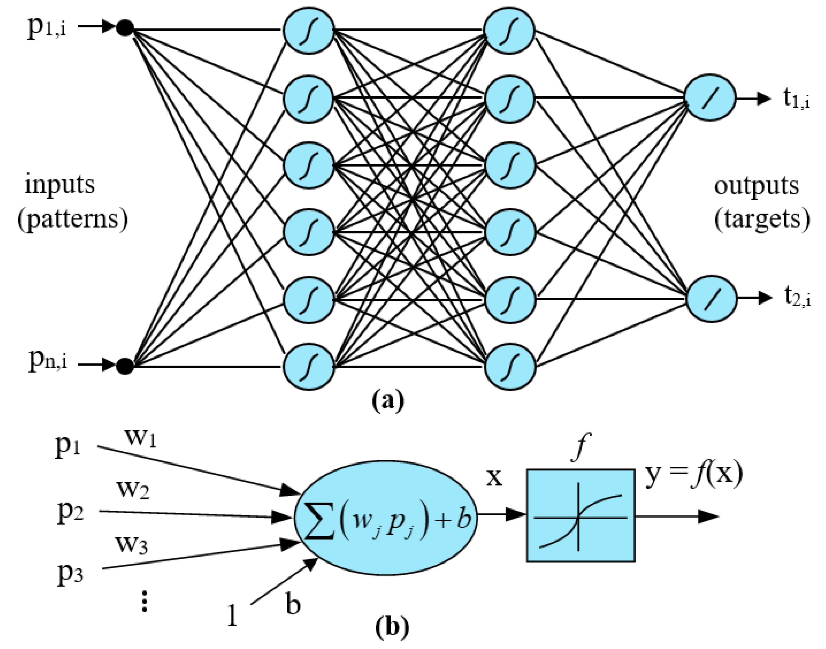
The multilayer perceptron neural network consists of a determined number of neurons, organized in two or more layers, highly interconnected [39]. The neuron operation consists of applying a determined transfer function to a weighted sum of its inputs. The MLP topology can be seen in Figure 4. It is usual the choice of a “tan-sigmoid” transfer function for hidden layers and a “linear” function for output layer.

The MLP network requires supervised learning. It uses a given set of input-output pairs for adjustment of the interconnection weights. The backpropagation learning algorithm is applied to adjust the weight array, W, associated with the interconnections. For each learning cycle, the ANN receives the input vectors (organized in the input matrix array containing the patterns, P). The resulting output vectors are compared to the desired outputs contained in the learning patterns (organized in the output matrix array containing the targets, T), and the performance index is calculated. This index is the mean squared error, “mse” [40], given in (15). Figure 4a shows the MLP with the inputs and outputs used in the training process. Figure 4b shows the operation of a neuron in any of the layers. The mathematical backpropagation algorithm determines the re-adjustment of the interconnection weights to reduce the mse. This cycle is iteratively repeated until the mse reaches a small enough value, previously given as the training goal.

The performance index, mse, taken as the accuracy goal whose value must be minimized, is defined as in (15):

$$mse=\frac{1}{m}{\displaystyle \sum _{i=1}^m{\Vert {\mathit{y}}_i-{\mathit{t}}_i\Vert }^2}$$

(15)

where m is the number of training patterns, and y_i, t_i, are the output and target vectors corresponding to the pattern i. The difference y_i − t_i is the error vector for that pattern, and ǁy_i − t_iǁ expresses the error vector length in the output space. In particular, with a two-neuron output layer, the output space is bidimensional. The sum of the squares of those error lengths, divided by m, gives the mean squared error, which is calculated after every iteration or epoch.

Among the different available backpropagation algorithms, the default algorithm applied in feedforward ANN training by the Neural Network Toolbox in MATLAB is the Levenberg–Marquardt algorithm, LM. It is also known as Damped Least-Squares, DLS. The authors have also tested other algorithms, such as the Scaled Conjugate Gradient, SCG. However, the best results were, in general, obtained with the LM algorithm.

The required number of neurons and neuron layers is selected after some tests of convergence. We have experienced with one, two, and three hidden layers.

The work stage after the training usually consists of some simulation tests to check the performance of the resulting network, evaluating its “generalization” capability. It consists of checking the ability of the ANN to give the correct output for input vectors different from those used for training.

3.2. Training for Fundamental Harmonic Detection

In [32], the MLP networks were trained to estimate the amplitude and phase of the main harmonics in distorted waveforms, from order 3 up to order 13. From these variables, the distortion component waveform was generated. This could be employed as compensation current, thus eliminating a part of the distortion. Besides, the patterns and training were based on a fixed 50 Hz fundamental frequency. The use of only few harmonics, and a fixed electric frequency, does not ensure an efficient operation for the typical nonlinear distortions. The ANN showed some potential for this kind of objective, but with limited and poor results. In [33], a comparative analysis was conducted between the application of the Adaline network and the MLP to obtain the reference signals for a shunt APF. The conclusion in that work is that the MLP performance is much lower than that of the Adaline method. However, in our opinion, the problem is with the inappropriate application strategy and training method.

In this work, the APF control method is based on the sampling of every waveform cycle of the current or voltage for the ANN input. A nominal 50 Hz electric frequency was considered. Nevertheless, the method should also work regardless of which electrical frequency is used. In the case of 50 Hz, after every time interval of 20 ms, the ANN outputs are the rectangular coefficients of the fundamental harmonic.

3.2.1. Patterns Generation

After a huge number of tests with different points per cycle and number of ANN inputs, a slow sampling rate of 2.5 kHz could be chosen, i.e., 50 points per waveform cycle, which means that the neural network must contain 50 inputs. For the strategy of extracting the fundamental harmonic, there was no need to increase the number of samples. It also works with faster sampling, but at the cost of increasing the size and complexity of the ANN, as well as the training times, without achieving higher performance.

Different harmonic spectrums of nonlinear loads were analyzed to choose suitable magnitudes of the different harmonics.

Table 1. Value intervals of the rectangular coefficients used in the generation of training patterns.

Coefficients	Training Intervals	Coefficients	Training Intervals
A1, B1	[−1, 1]	A11, B11	[−0.1, 0.1]
A3, B3	[−0.6, 0.6]	A13, B13	[−0.1, 0.1]
A5, B5	[−0.2, 0.2]	...	...
A7, B7	[−0.2, 0.2]	A33, B33	[−0.01, 0.01]
A9, B9	[−0.2, 0.2]	A35, B35	[−0.01, 0.01]

shows the intervals of values allowed for the rectangular coefficients of the odd harmonics, up to the 35th, used in the training patterns. The determination of the suitable harmonics and amplitudes was also the result of a long process, based on the authors experience and the trial-and-error method.

An important requirement for the control method is to maintain its performance in case of electric frequency deviations from the nominal value of 50 Hz. A robust behavior of the ANN requires the use of different fundamental frequencies in the training patterns. In some previous tests, we could observe that an ANN trained only with 50 Hz does not work properly in practical cases due to the possible frequency deviations of the supply voltage. Therefore, the patterns were generated using five different values of frequency between 49.5 and 50.5 Hz.

A key feature enabling the required MLP learning has been the use of random combinations of harmonics. Initially, we generated high amounts of patterns in determined manners, without obtaining a low enough mse. Then, using the MATLAB function “unidrnd” it was possible to randomly generate any number of patterns: A₁ = (unidrnd(5,1,1)-3)*0.5; B₁ = (unidrnd(5,1,1)-3)*0.5; A₃ = (unidrnd(5,1,1)-3)*0.3; and so on, up to B₃₅. This operation gives, for A₁, random values from the set {−1, −0.5, 0, 0.5, 1}. This approach provided a very efficient set of patterns. For every different frequency, an amount of 20,000 combinations of harmonics were generated, providing an input matrix P of size 50 × 100,000. The size of the desired targets matrix T is 2 × 100,000, containing the A₁ and B₁ values of every waveform.

3.2.2. Design, Training and Testing

After many tests with different combinations of hidden layers and neurons per layer, the best configuration found was 50-10-10-2. That is, 50 input units, 2 hidden layers containing 10 neurons each, and the 2-neuron output layer. The transfer functions are tan-sigmoid in the hidden layers, and linear in the output one. These decisions were based on the authors’ experience and on many trials, reducing the number of neurons as much as possible. This allows us to increase the number of patterns used in the learning process, without excessively long training times.

Both the LM and the SCG backpropagation algorithms were used for training, but in general, the LM algorithm allowed us to achieve lower values of the goal mse parameter. After a training of 100 epochs with LM, a value of mse = 2·10⁻⁷ could be reached. The SCG method carried out thousands of epochs in the same time intervals, yet it did not reach the same low errors. So, the definitive ANN used was trained with LM. Concerning the conditions to end the last and definitive training, the key aspect is to observe the evolution of the mse with the increase in the number of epochs. Once we knew that in different trials, the mse value stopped decreasing after 80 or 90 epochs, taking values around 2·10⁻⁷, we set a number of 100 epochs as training limit, and run the last training.

After training the ANN, the generalization capabilities and the accuracy of the outputs were checked. For these performance tests, we generated a high number of waveforms with random combination of the different harmonics and different fundamental frequency values. Many of these inputs included coefficients A_i and B_i exceeding the limits shown in Table 1. In addition, the fundamental frequency was used, exceeding the limits applied by the pattern generation. In particular, frequencies from 45 to 55 Hz were tested. The results of the generalization tests were satisfactory, proving that the ANN was accurate enough to be used in practical cases of three-phase systems.

4. Results in Practical Cases

In order to quantify the results obtained with the ANN-APF, two essential indices were used: the total harmonic distortion of the supply current, ITHD, defined in (16), and the power factor, PF, defined in (17), measured before and after compensation.

$$ITHD=\frac{\sqrt{{\displaystyle \sum _{i\hspace{0.17em}>\hspace{0.17em}1}{I}_i^2}}}{I_1}\hspace{0.17em}\cdot \hspace{0.17em}100\%$$

(16)

$$PF=\frac{P}{\sqrt{V_a^2+V_b^2+V_c^2}\sqrt{I_a^2+I_b^2+I_c^2}}$$

(17)

Those indices, together with the monitoring of the voltages and currents waveforms, will allow us to evaluate the system performance. In addition, international standards were taken into account: IEC 61000-4-30 [41] and EN-50160 [42]. Thus, it is strongly recommended to achieve a source current ITHD below 5% and a PF close to one. In that sense, the control system will be required to operate in the environment of 50 Hz ±1%, i.e., from 49.5 to 50.5 Hz, as this is the interval in which the frequency must be during 95% of the time every week. Obviously, it is also desired that no important disturbance would be observed in case of higher frequency deviations. The standard requires the electrical network to work 100% of the time in the interval from 50 − 6% to 50 + 4%, i.e., from 47 to 52 Hz [41].

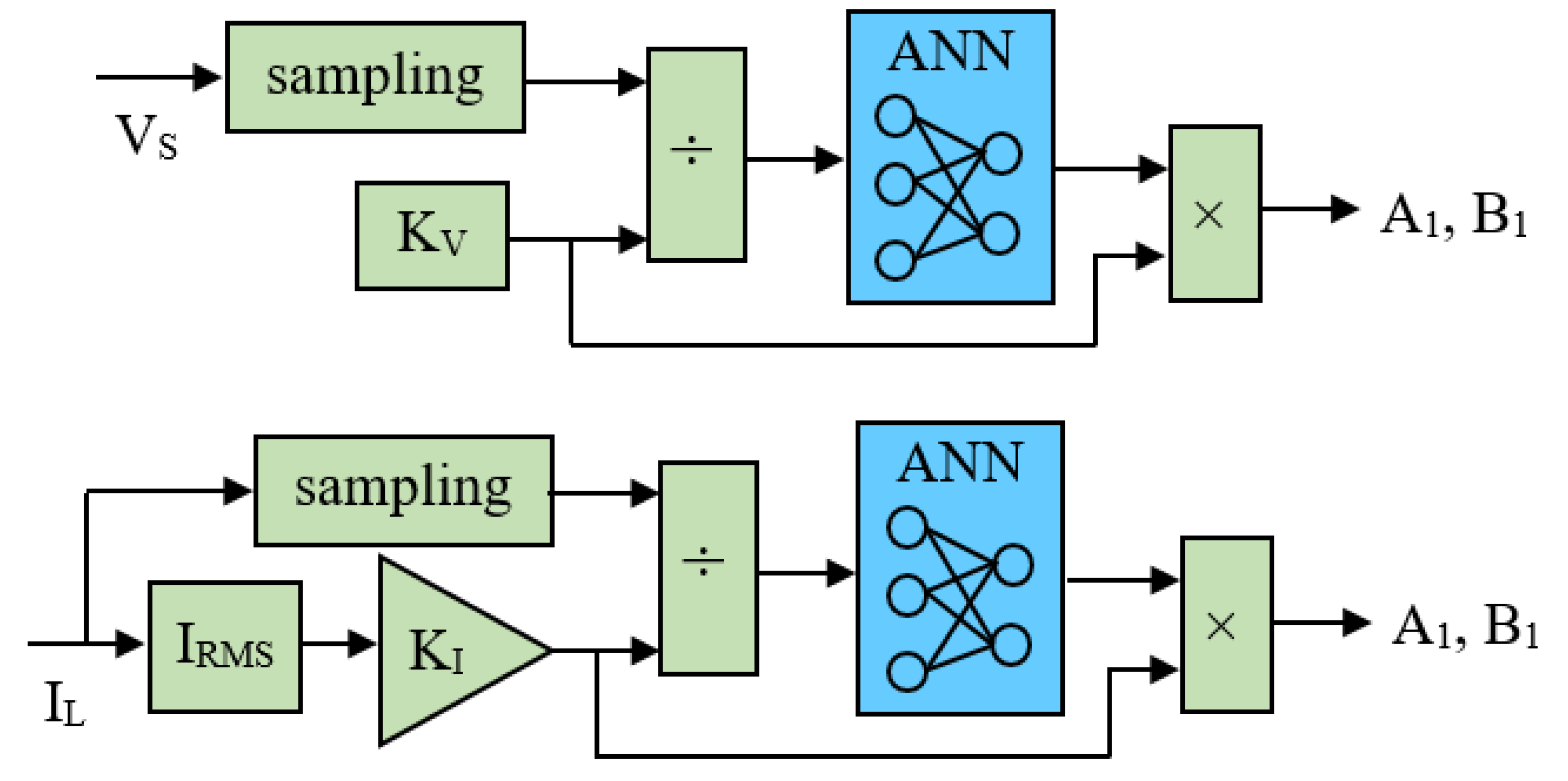
In order to use the neural networks with currents and voltages of practical three-phase circuits, a scale factor must be applied to the waveforms before accessing the ANN, because their amplitudes can reach values of several Amperes and hundreds of Volts. The generalization capability tests showed a wide tolerance for input waveform amplitudes. However, the ANN performance is higher if the input waveforms do not significantly exceed the ±1 range.

In the practical cases, the voltage waveforms have amplitudes over 300 V, whereas the fundamental harmonic amplitude in the waveform patterns was not higher than sqrt (1² + 1²) ≈ 1.414. Therefore, the voltage inputs were divided by a scale factor K_V before reaching the ANN, and consequently, the outputs must be multiplied by the same factor. Figure 5 shows the required adjustment of the inputs and outputs.

For the same reason, current inputs need the application of a scale factor. Considering the dependency of the currents on the variable loads, the scale factor was based on the measurement of the load current rms value. The product K_I·I_RMS has provided an autonomous adjustment of the scale factor. In particular, values of K_I = 0.4 or 0.5 were appropriate. The current data are divided by K_I·I_RMS and the ANN output is multiplied by the same factor. Figure 5 shows this input and output adjustment.

No special stability analysis was conducted. On one side, the feedforward ANNs have no feedback connections, and do not use online training algorithms to adjust any parameter. The ANNs use the load current signals (independent of the SAPF injected currents) to obtain, after every cycle, the coefficients A and B for generation of the reference signals. This absence of feedback loop can contribute to a stable behavior. On the other side, the hysteresis PWM control and the use of inductors in the connection of the APF with the three-phase system usually do not cause unstable operation. If the ANN control does not obtain correct coefficients in some of the cycles, the APF could produce some short time intervals without a perfect compensation. However, the way in which the ANN refreshes the outputs after each cycle should avoid any rare cumulative effect or stability problem. Therefore, no concerning SAPF unstable operation should be expected. All practical cases tested in this work presented stable operation.

4.1. Results by Simulation Practical Cases

Some MATLAB Simulink models have been designed to test the operation of the neural control of the APF in several cases, including different loads, frequency deviations, and step changes in the load.

Both compensation objectives described in Section 2 were tested: HC and UpfC. The common objective of reducing the harmonic distortion was analyzed by measurement of the ITHD, which is desired to reach values under 5%, whereas the UpfC control method is expected to achieve a PF close to unit, in addition to the low ITHD.

Table 2. Main electric system parameters of the test models.

Parameters of the System Setup	Value
V source	400 V
Nominal frequency	50 Hz
Three-phase load impedance	30 Ω, 40 mH, series
AC regulator thyristors	firing angle 90°
Filter series inductance	18 mH
Inverter control	hysteresis band ± 0.03
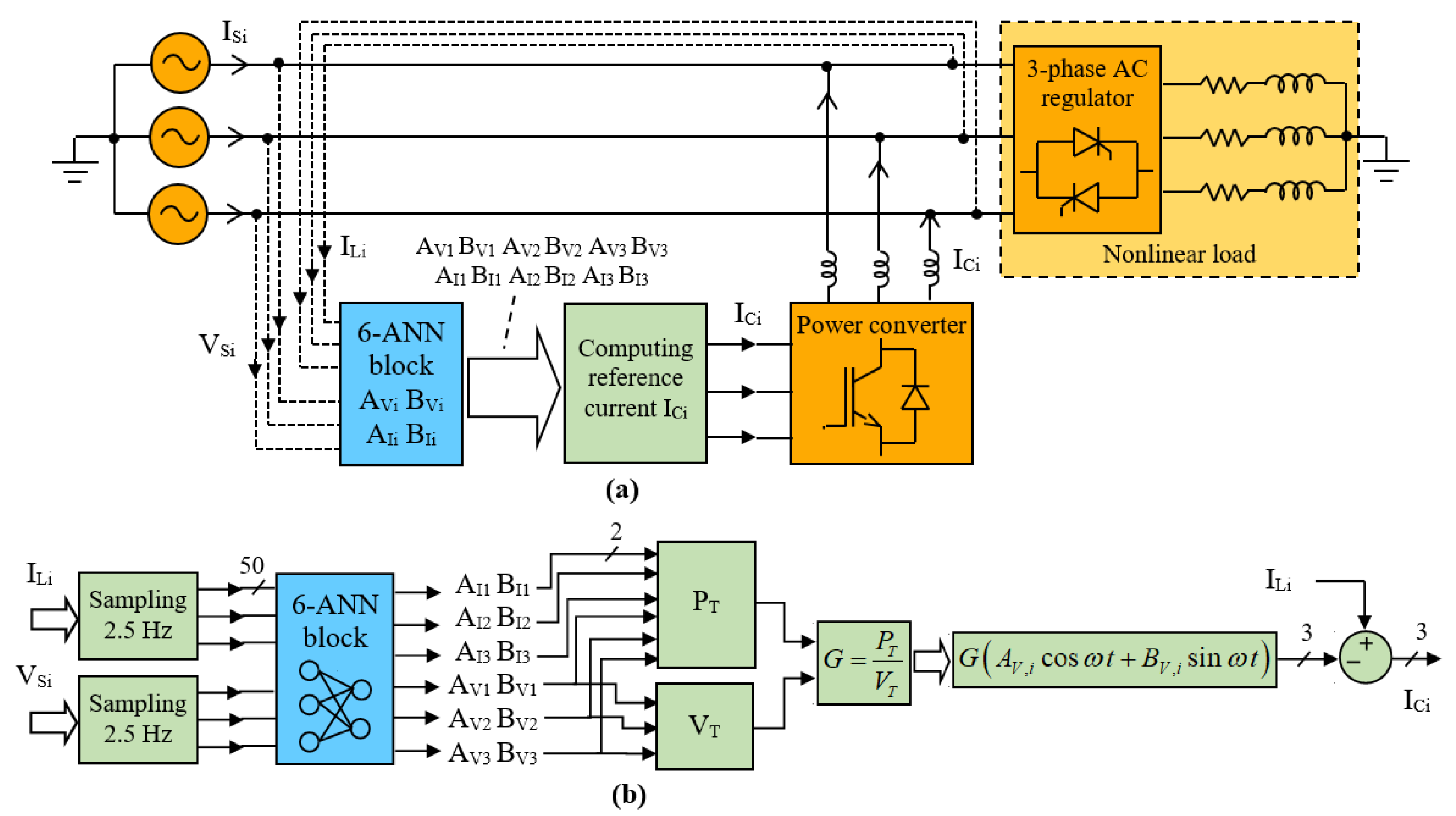
Sampling frequency	2500 Hz

shows the most relevant parameters of the electric system and APF used in the simulation models. The nonlinear load consists of a set of impedance branches connected to AC regulators based on thyristors, as shown in Figure 3a.

4.1.1. HC Control Method Simulation Results

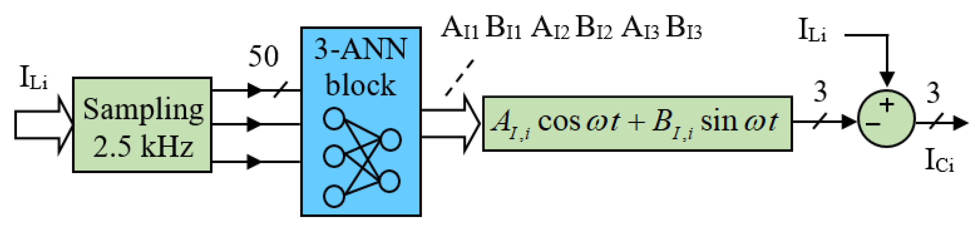
The first practical case is based on the HC method according to operation in (6), shown in Figure 2. The use of three ANNs, working in parallel, allows us to obtain the fundamental components of the phase currents. The subtraction of these components from the load currents gives the reference signals for the power converter. This test was carried out with a 50 Hz frequency and a load consisting of a three-phase thyristor regulator with firing angle of 90°, followed by RL series branches with values shown in Table 2.

Figure 6 shows the load and source currents resulting in this case. Whereas the load ITHD is 43%, the value at the source is reduced to 2.4%.

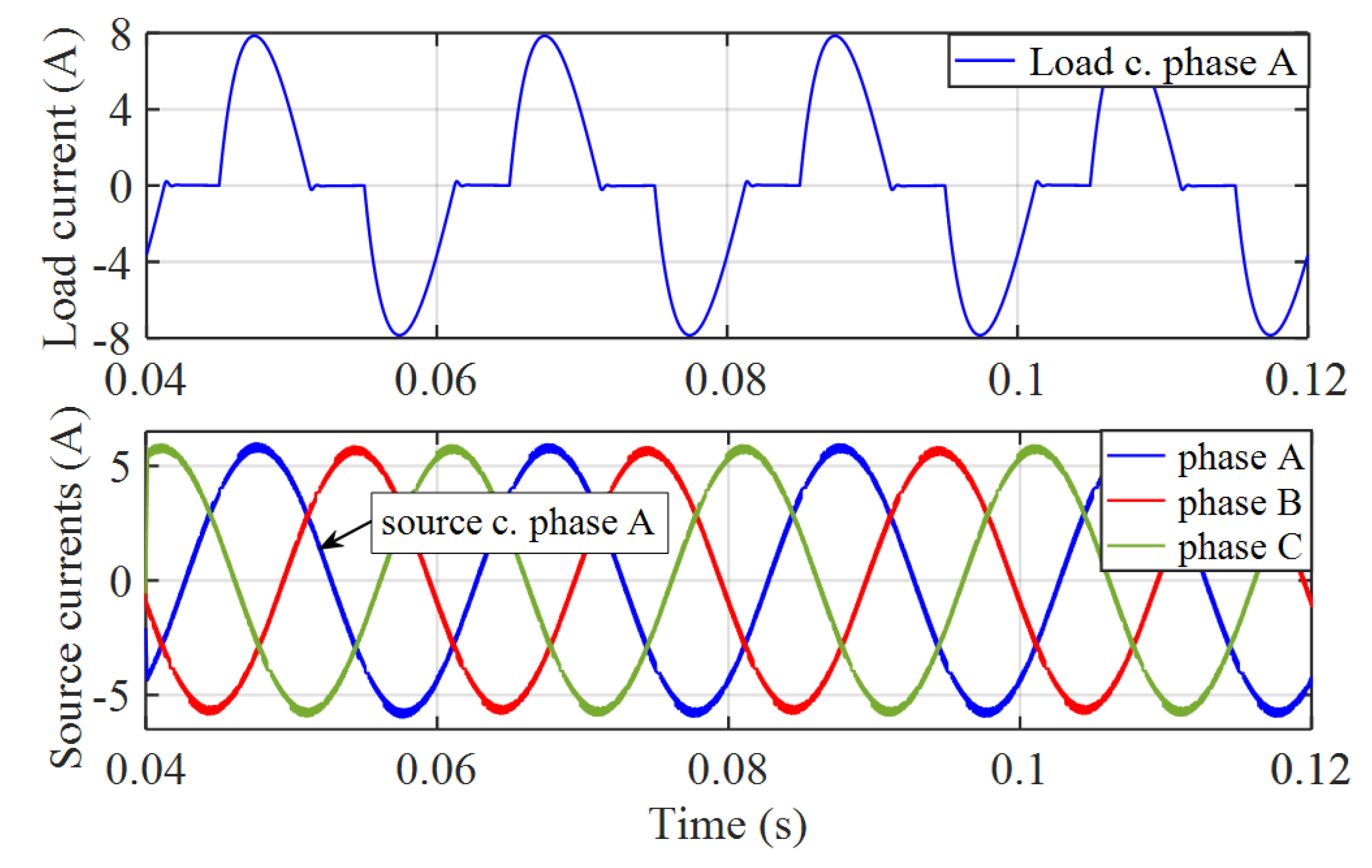
Another test was carried out to analyze the dynamic response in case of load change. The connection of an additional load in parallel with the former nonlinear one shown in Figure 3a was established at time t = 0.08 s. It is a linear load consisting of RL series branches of values 60 Ω and 80 mH. Figure 7 shows the resulting waveforms, where it can be seen that two electric cycles after the change, the source currents reach the new steady state. The load ITHD after the change is 24%, and 1.7% for the source currents. The system behavior for some other tested changes showed similar performance.

4.1.2. UpfC Control Method Simulation Results

The next step is the simulation of practical cases based on UpfC control where a more complete compensation is searched. According to (13) and Figure 3, this objective requires in general the use of six ANNs for the estimation of the rectangular coefficients A_I,i, B_I,i, A_V,i and B_V,i. In addition, a different computation block is used after the work of the ANNs, as described in Section 2 and Appendix A, and shown schematically in Figure 3b.

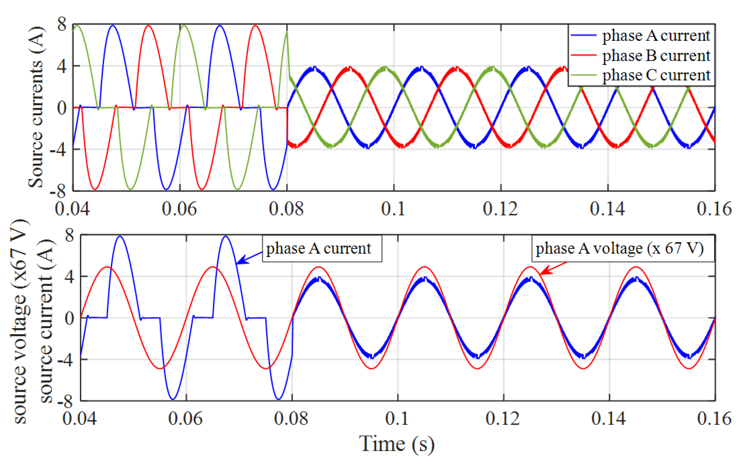
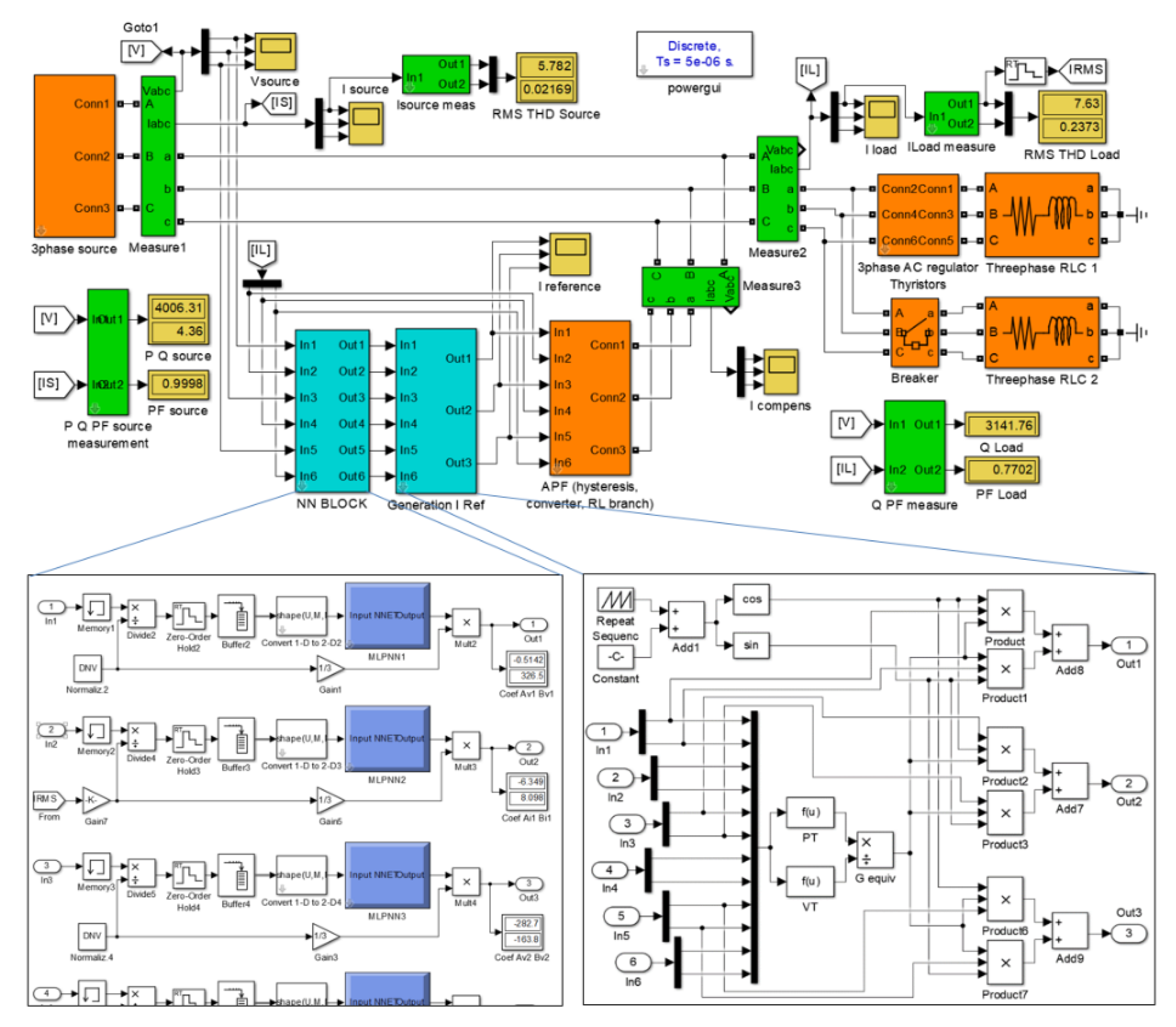
The same system parameters of Table 2 were used. The waveforms in Figure 8 show the results, before and after the connection of the shunt APF at time t = 0.08 s. The source currents become sinusoidal and in phase with the voltages. The ITHD is reduced from 43% to 3.7%, improving the PF from 0.583 to 0.9993. Figure 9 shows the Simulink model for this compensation strategy.

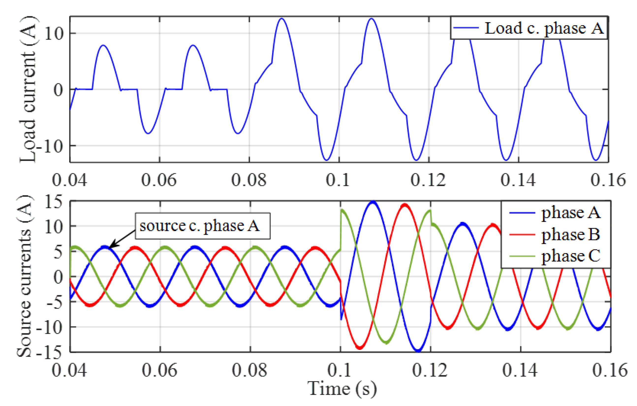
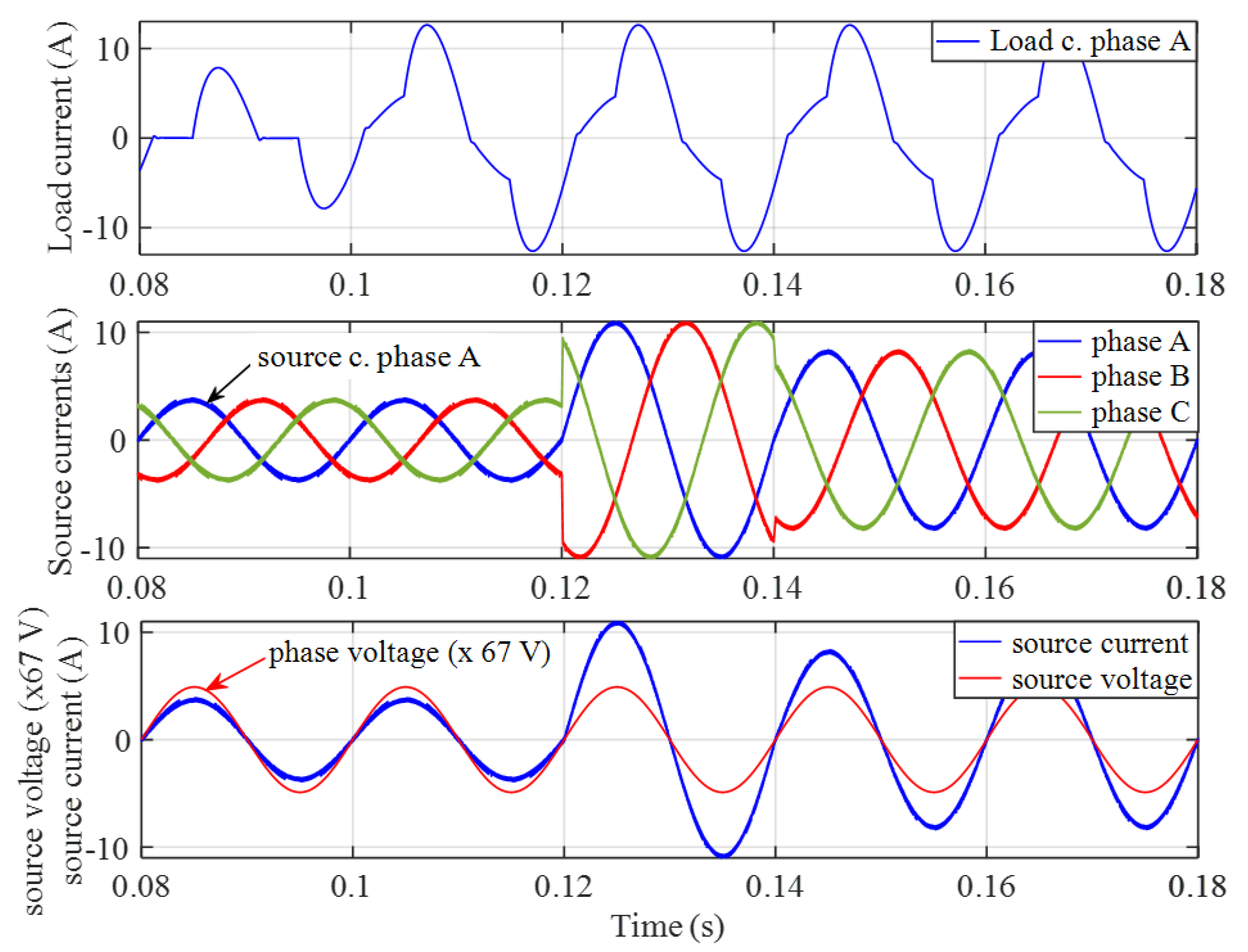
Next, some tests were carried out to observe the dynamic response in case of load changes. Two different changes were applied. In the first test, whose Simulink model is shown in Figure 9, a linear load was connected in parallel with the nonlinear one of Figure 3a or Figure 9, at t = 0.1 s, with the same values of R and L as in the former subsection. Figure 10 shows the results. It can be seen that after two cycles, the source currents recover the steady state sinusoidal waveforms, in phase with the voltages. The ITHD after the change is 24% for the load currents and 2.2% for the source currents. The current values after the change are 7.63 A at the load and 5.78 A at the source. The PF is 0.7702 at the load and 0.9998 at the source.

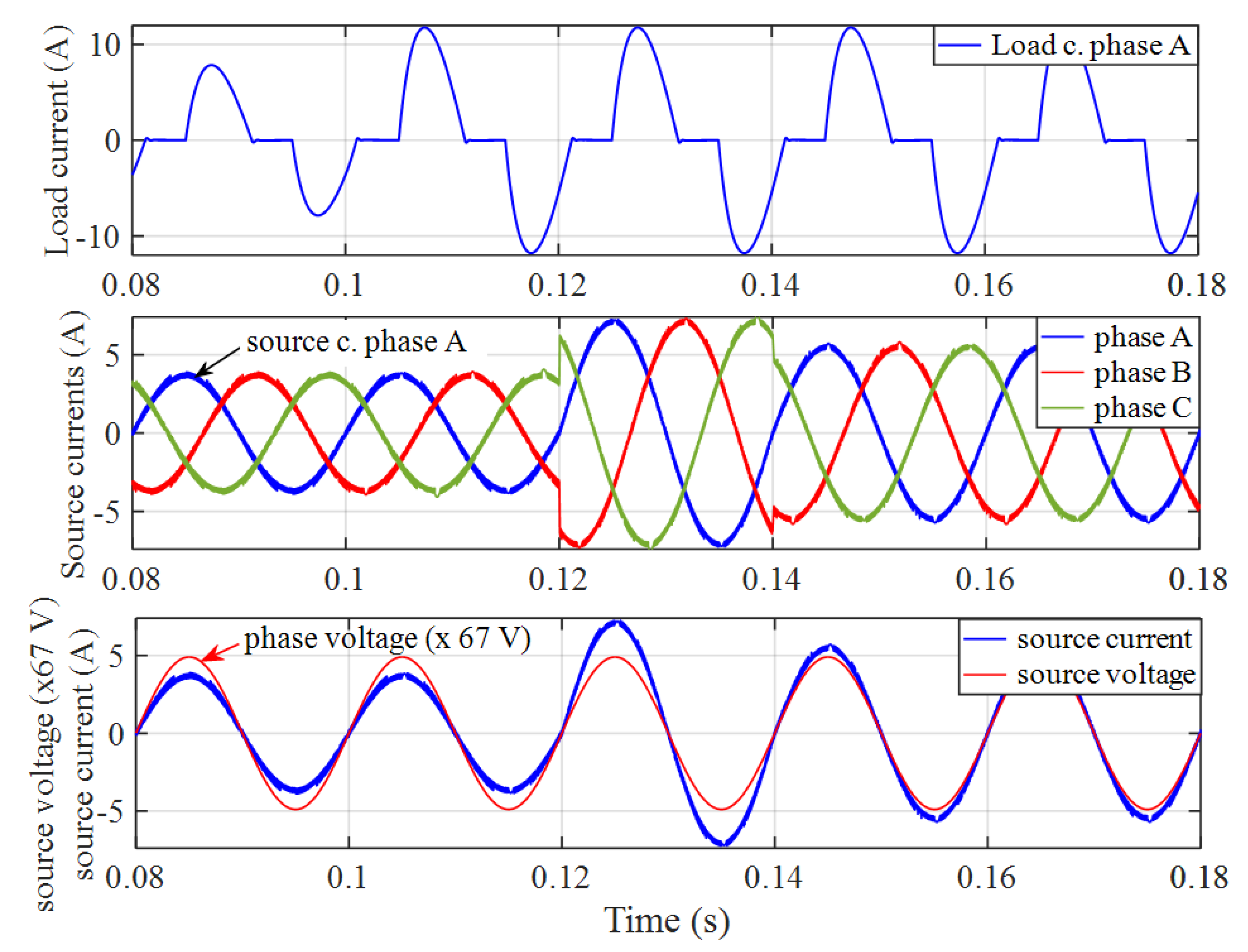
In the second load change tested, an increase in the nonlinear load was applied, connecting a new RL load in parallel with the RL branches of Figure 3a, behind the thyristors’ regulator. Figure 11 shows the waveforms. Again, after a short transient, the source currents recover the desired stationary state with sinusoidal waveforms, in phase with the voltages. The ITHD after the change is 43% for the load currents and 3.3% at the source. The current values are 6.69 A at the load and 3.90 A at the source. The PF is 0.5828 at the load and 0.9994 at the source.

Some of the Adaline-based control methods show that the time interval to recover stationary state after a change is around one quarter of a cycle [11,12]. In [12], they have proven that among the different tested methods, this is the fastest response observed, while some other control methods require several cycles. For example, one of the recent control methods with good general results, as is the case of [23], using the NARX neural network, requires more than five cycles after the load change. Hence, we can affirm that the two-cycle interval observed in this work is not a high amount of time.

4.1.3. UpfC Tests by Frequency Deviations

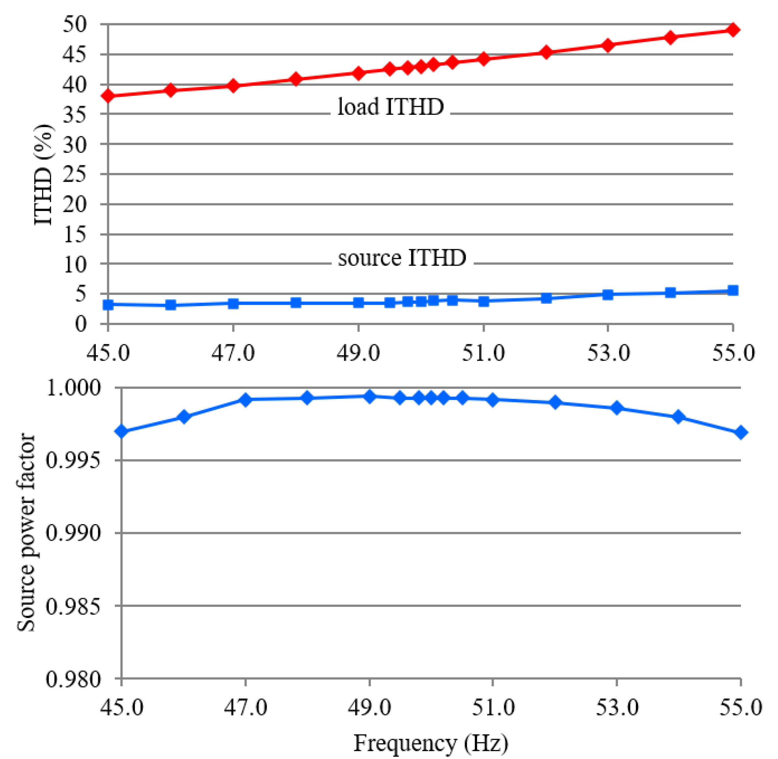
One of the relevant objectives of this work was the robust behavior of the control system under the contingency of frequency deviation. For the ANN training, the distorted waveform patterns included different fundamental frequency values. The UpfC control performance was tested in two different ways. In the first test, the performance of the compensation system was analyzed in a range of frequencies between 45 and 55 Hz, in terms of ITHD and PF. In the second test, the dynamic response was evaluated in case of frequency changes during system operation.

With the same system parameters of Table 2, the measurements for different frequencies were established. In previous subsections, with a 50 Hz frequency, it has been reported that the load ITHD was 43% and the PF was 0.583. Now, it can be observed in Figure 12 the graphical results of ITHD and PF versus frequency. The load ITHD is high for every frequency, but the source ITHD remains under 5%, with values under 4% inside the important interval proposed by the IEC Standard [31], from 47 to 52 Hz. Regarding the PF achieved, the values are very close to unity, over 0.997 in the whole frequency interval, and over 0.999 in the interval from 47 to 52 Hz.

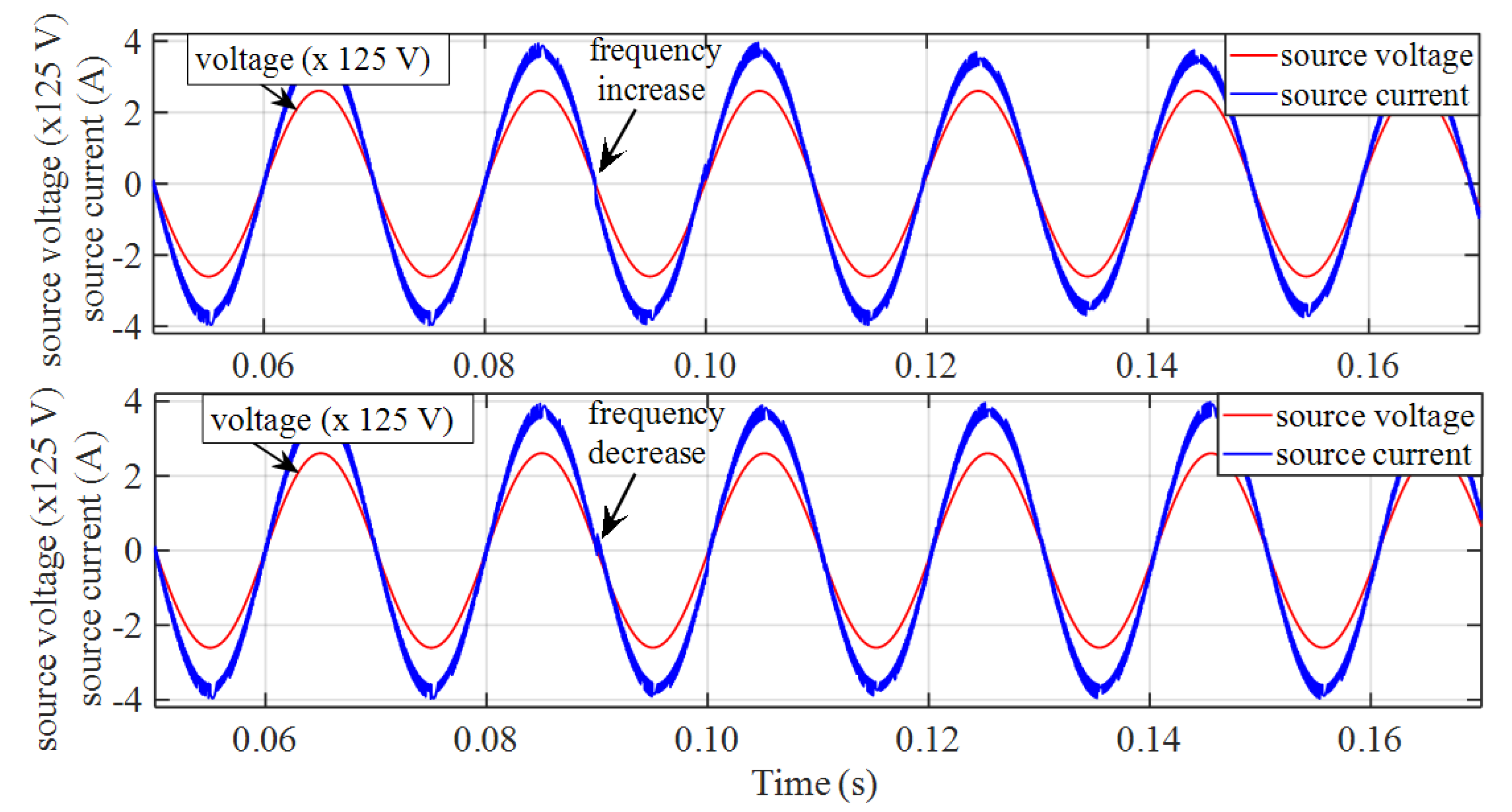
In the second test, step changes of 0.5 Hz were applied during system operation. In particular, Figure 13 shows the behavior for an increase from 50 to 50.5 Hz at t = 0.09 s, and a decrease from 50 to 49.5 Hz at t = 0.09 s. The source current reaches steady state after one cycle.

In conclusion, the UpfC control performance is robust enough under frequency deviations. It achieves the required compensation inside a wide frequency range and can respond quickly to the frequency changes.

4.2. Experimental Results

Harnessing the potential of ANNs requires their implementation in a specific integrated circuit. However, a laboratory setup based on data acquisition cards has allowed for a first experimental validation in obtaining compensation currents with ANNs. Thus, a modular system based on dSpace cards was developed. Specifically, the set includes a DS1005 PPC control card developed from a PowerPC 750GX 1 GHz processor that runs the control program in real time. This card manages the inputs and outputs from/to the power system through a DS2004 card with 16 input channels, and a DS5101 DWO card with 16 TTL pulse outputs. The input signals to the DS2004 card are from a set of Hall effect LEM sensors: LV-25-P sensors for voltage signals and LA35-NP sensors for current signals. The APF power circuit consists of a three-phase inverter with IGBTs, the Semikron SKM50GB123D. It is a three-leg inverter with two capacitors on the DC side at whose midpoint the neutral connection can be made. More details on the experimental prototype can be found in [2].

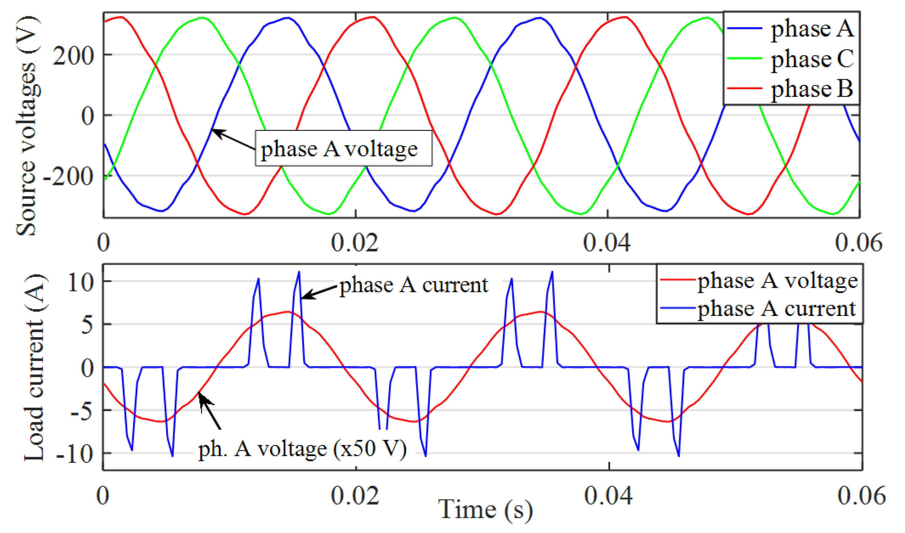
A three-phase diode rectifier with capacitive filtering on the DC side was connected to the 400 V, 50 Hz distribution network (230 V phase voltage). This frequently constitutes the input circuit of a variable speed drive of an asynchronous motor. Figure 14 shows the phase voltage waveforms of the grid, which present the distortion and unbalance typical of a low voltage supply. It also shows the voltage and current of the load for the same phase (phase a), where it can be observed the high current distortion corresponding to an ITHD of 144%.

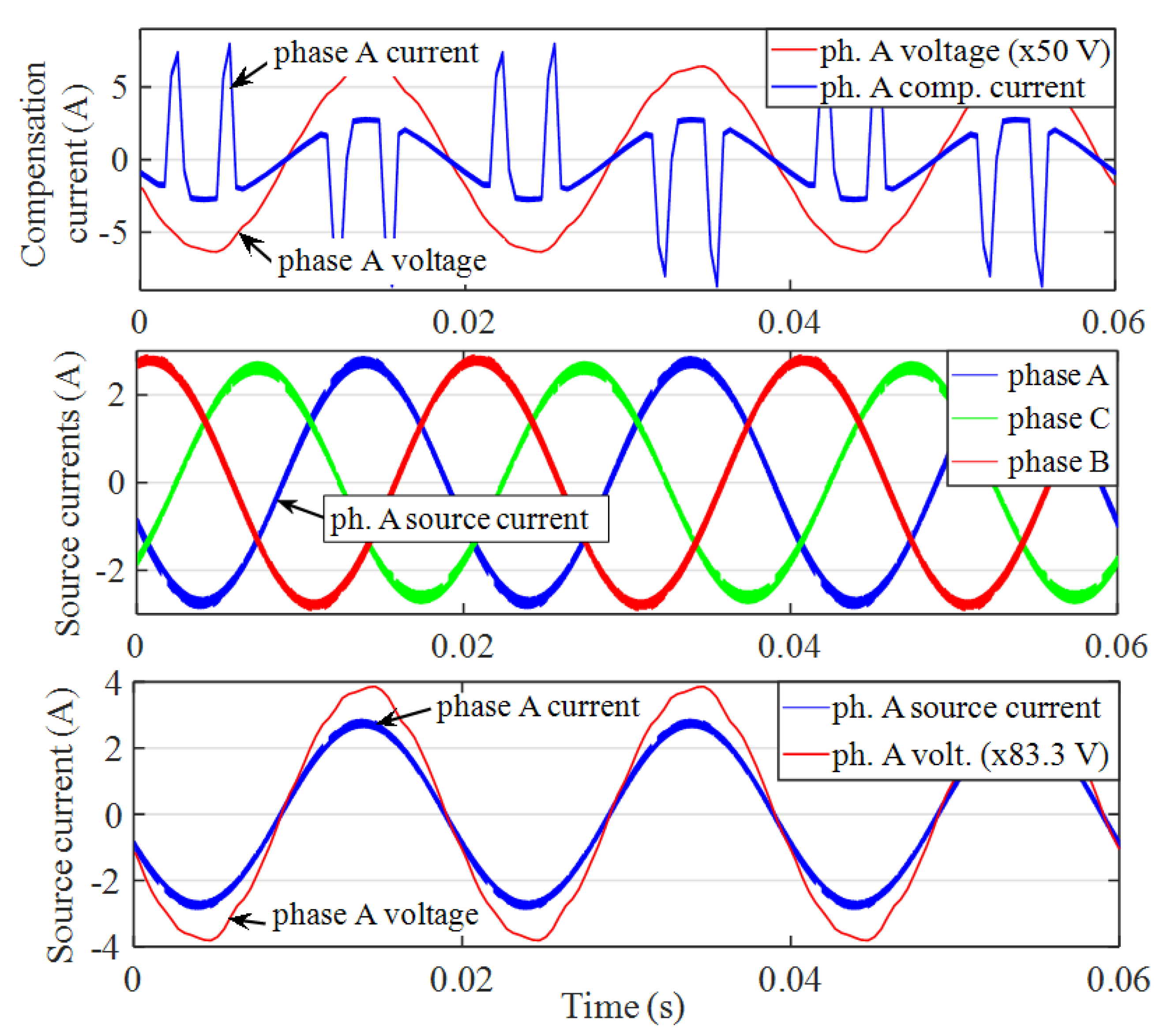
The UpfC strategy was executed on the control card, which has allowed determining the compensation currents. Figure 15, upper graph, shows the compensation current generated by the ANN control circuit. The middle graph shows the resulting sinusoidal source currents, where the ITHD value is 3.9%. Finally, Figure 15, bottom graph, contains the supply voltage and current waveforms in the same phase after compensation. As a result, theses voltages and currents are collinear, reaching a power factor close to unity.

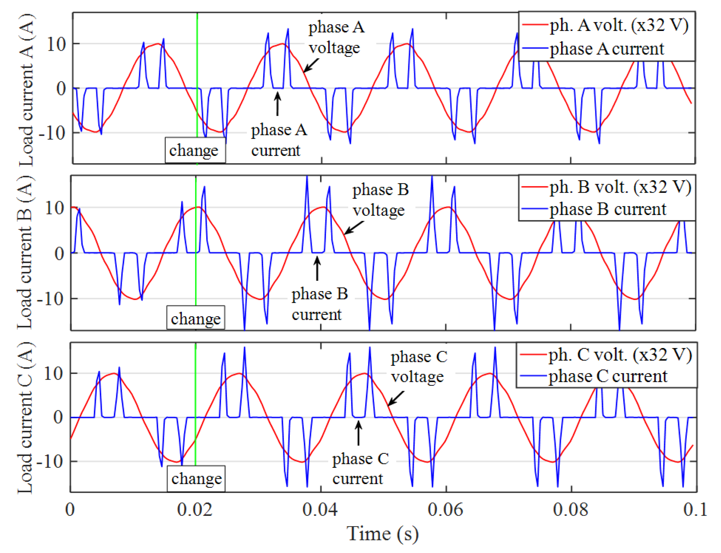
The unbalanced load performance was also tested. According to (8), the UpfC strategy will produce source currents proportional to the source voltages. Therefore, in most real cases, where not much voltage unbalance is present, the compensation will give rise to balanced three-phase source currents. Figure 16 shows a load change from the previous load features to lower impedance values, and different for each phase. Thus, the current amplitudes become higher and show some unbalance. The load ITHD is over 140% in every phase.

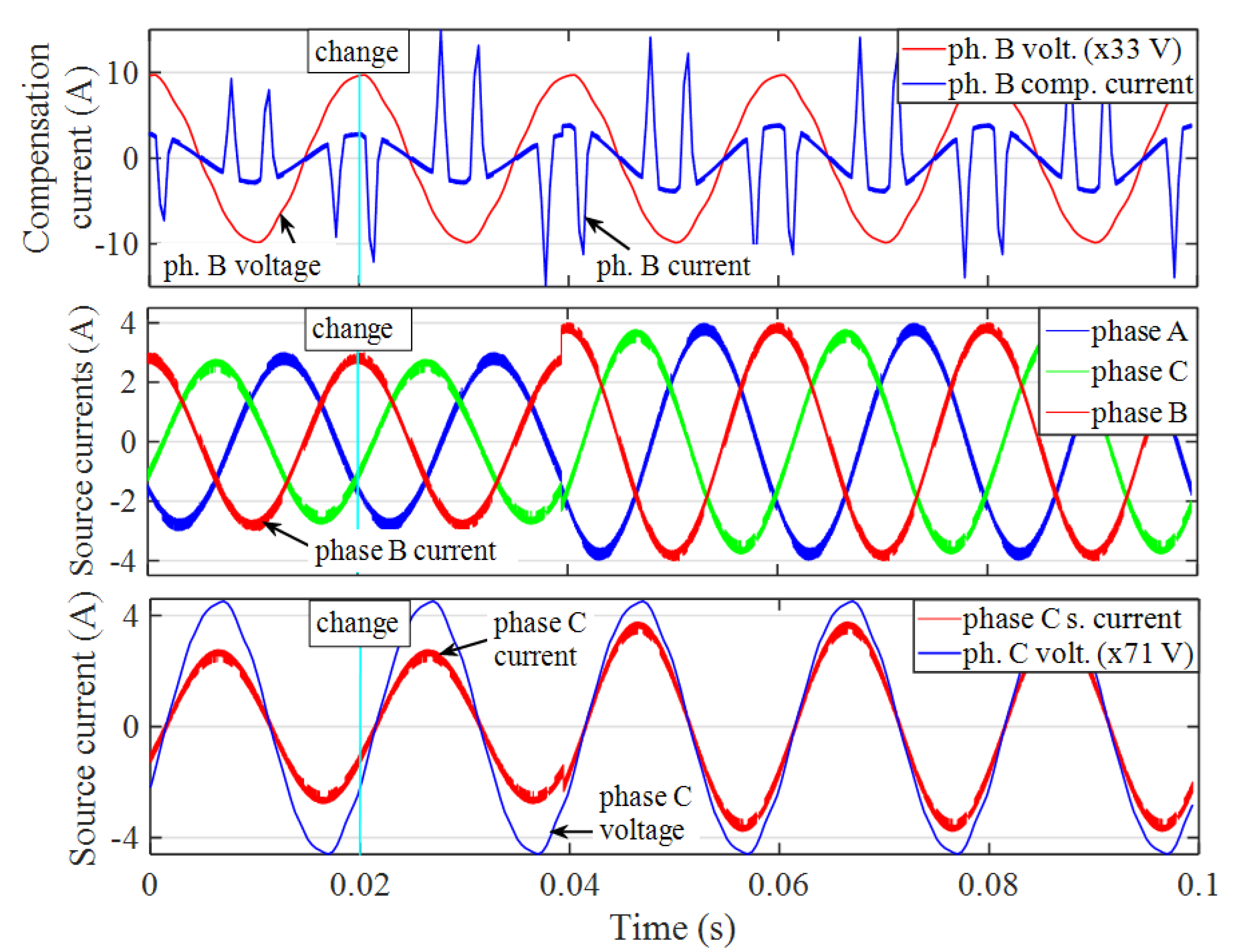
In Figure 17, the UpfC compensation results are presented. The top graph shows the compensation current in one of the phases. The middle graph shows the sinusoidal source currents, with the correction one cycle after the change, becoming quickly stationary and almost balanced. The slight unbalance that can be appreciated is due to the small voltage unbalance. The source ITHD values fall into 4.0%, 4.1%, and 3.8% for the phases a, b, and c, respectively. Finally, Figure 17, bottom graph, contains the supply voltage and current waveforms, which highlights the power factor correction.

After all these tests were carried out, it is important to highlight some relations with the reference works. The source ITHD values achieved in this work, as in the best of the Adaline or RNN works reviewed, are between 2% and 5%. The PF reached in these cases is unity. The dynamical performance is as good as in many of the accepted control methods. Lastly, the UpfC control strategy corrects the problem of unbalanced currents, in the case of balanced source voltages.

Table 3. Some features of the reference works, with control methods based on different ANN types.

ANN Type, Reference	Applied to APF	Source ITHD <5%	Power Factor Compensation	Balanced Source Currents	Experiment Results	Dynamical Tests	Frequency Deviations Test
ADA [11]	✓	✓	✗	✗	✓	✓	✗
ADA [14]	✓	✓	✗	-	-	✓	✓
ADA [16]	✓	✓	✓	✗	✓	-	-
RBF [19]	✓	✓	✗	✗	✗	✓	✗
RBF [20]	✓	✓	-	✓	✗	✓	✗
RNN [21]	✓	✓	✗	✗	✗	✓	-
RNN [22]	✓	✓	✗	✗	✓	✓	-
NARX [23]	✓	✓	✓	✓	✗	✓	✓
ESN [25]	✓	✓	✓	✓	✓	✓	✗
MLP [32]	✗	(1)	-	-	✗	✗	✗
MLP [33]	✓	✗	✗	✗	✓	-	-
This work	✓	✓	✓	✓ (2)	✓	✓	✓

⁽¹⁾ This method estimates a 4.4–6% ITHD value for the waveform resulting of subtracting the harmonic waveform from the distorted load current, but without real compensation. ⁽²⁾ It works in the case of balanced supply voltages.

shows a summary of some important features of different ANN-based control methods in the literature included as references in this paper.

In the comparison of some reference works showed in Table 3, it can be seen that most of the methods achieve an ITHD value below 5%, recommended by the EN Standard [42]. Regarding the other features showed in the table, we can affirm that the method proposed in this paper reaches a complete set of requirements.

In future works, this MLP-based control method must be further tested in the experimental platform with different loads and adverse conditions for an in-depth analysis of the performance. Besides, it is important to try to apply new deep learning techniques and other new ANN topologies, maintaining the control strategies and testing platforms for comparison.

5. Conclusions

A new control method for the three-phase shunt active power filters has been proposed for harmonic and reactive power compensation. Over the years, many control strategies based on artificial neural networks have been tested. However, the simple and extended feedforward or multilayer perceptron ANN could not be successfully applied as the core element of an APF control. In this work, the search for an appropriate MLP application strategy and an in-depth training with distorted waveforms allowed us to prove that this ANN topology is a feasible alternative. An MLP containing two hidden neuron layers (10-10-2 neurons) was used for inputs consisting of the samples of every waveform cycle and outputs consisting of the fundamental harmonic Fourier coefficients, A₁ and B₁. Six identical ANNs estimate the coefficients of fundamental currents and voltages. The computation method described in the work allows us to obtain the compensation currents from these coefficients. The 100 thousand waveform patterns for the training were generated through random harmonic combinations, including high order harmonics and variable fundamental frequency. The MLP learning, with mse around 2·10⁻⁷, was enough to reach accurate fundamental harmonic waveforms of currents and voltages in any practical three-phase system, even in the case of frequency deviations in the interval from 47 to 52 Hz, in compliance with the IEC standards. The compensation strategies were applied in practical cases implemented in a first stage with MATLAB-Simulink. After that, the method was also tested in an experimental prototype. Features such as source ITHD below 5%, unit power factor, good dynamic performance, and balanced source currents validate the proposal.

References

1. Akagi, H.; Watanabe, E.; Aredes, M. Shunt active filters. In Instantaneous Power Theory and Applications to Power Conditioning, 2nd ed.; Wiley-IEEE Press: New York, NY, USA, 2017; Chapter IV; pp. 111–236. [Google Scholar]
2. Salmerón, P.; Pérez, S.; Prieto, J. Shunt active power filter. In Active Power Line Conditioners: Design, Simulation and Implementation for Improving Power Quality; Elsevier: Amsterdam, The Netherlands, 2016; Chapter IV; pp. 107–146. [Google Scholar]
3. Baszynski, M.; Sowa, K.; Pirog, S. An active power filter with energy storage and double DC conversion for power surge compensation. Electronics 2020, 9, 1489. [Google Scholar] [CrossRef]
4. Hoon, Y.; Radzi, M.; Amran, M.; Zainuri, M.; Atiqi, M.A.; Zawawi, M.A.M. Shunt active power filter: A review on phase synchronization control techniques. Electronics 2019, 8, 791. [Google Scholar] [CrossRef] [Green Version]
5. Fei, J.; Wang, H.; Cao, D. Adaptive backstepping fractional fuzzy sliding mode control of active power filter. Appl. Sci. 2019, 9, 3383. [Google Scholar] [CrossRef] [Green Version]
6. Torabi, S.; Ghambari, M.; Mahmoudian, M.; Najafi, A.; Rodrigues, E.; Pouresmaeil, S. A novel control strategy to active power filter with load voltage support considering current harmonic compensation. Appl. Sci. 2020, 10, 1664. [Google Scholar] [CrossRef] [Green Version]
7. Eid, A.; Abdel-Salam, M.; El-Kishky, H.; El-Mohandes, T. Active power filters for harmonic cancellation in conventional and advanced aircraft electric power systems. Electr. Power Syst. Res. 2009, 79, 80–88. [Google Scholar] [CrossRef]
8. Salmerón, P.; Vázquez, J. Practical design of a three-phase active power-line conditioner controlled by artificial neural networks. IEEE Trans. Power Deliv. 2005, 29, 1037–1044. [Google Scholar] [CrossRef]
9. Tey, L.H.; So, P.L.; Chu, Y.C. Adaptive neural network control of active filters. Electr. Power Syst. Res. 2005, 74, 37–56. [Google Scholar] [CrossRef]
10. Dai, W.; Day, Y.; Wu, M. A new study for harmonic suppression and reactive power compensation. In Proceedings of the 2008 IEEE International Conference on Industrial Technology, Chengdu, China, 21–24 April 2008; pp. 1–6. [Google Scholar] [CrossRef]
11. Bhattacharya, A.; Chakraborty, C. A shunt active power filter with enhanced performance using ANN-based predictive and adaptive controllers. IEEE Trans. Ind. Electron. 2011, 58, 421–428. [Google Scholar] [CrossRef]
12. Merabet, L.; Saad, S.; Abdeslam, D.O.; Merckle, J. Direct neural method for harmonic currents estimation using adaptive linear element. Electr. Power Syst. Res. 2017, 152, 61–70. [Google Scholar] [CrossRef] [Green Version]
13. Hoon, Y.; Amran, M.; Radzi, M.; Al-Ogaili, A.S. Adaptive linear neural network approach for three-phase four-wire active power filtering under non-ideal grid and unbalanced load scenarios. Appl. Sci. 2019, 9, 5304. [Google Scholar] [CrossRef] [Green Version]
14. Vardar, K.; Akpinar, E.; Sürgevil, T. Evaluation of reference current extraction methods for DSP implementation in active power filters. Electr. Power Syst. Res. 2009, 79, 1342–1352. [Google Scholar] [CrossRef]
15. Das, S.R.; Ray, P.K.; Mohanty, A. Improvement of power quality using advanced artificial neural network algorithm. In Proceedings of the 2018 IEEE International Conference on Power Electronics, Drives and Energy Systems (PEDES), Chennai, India, 18–21 December 2018; pp. 1–6. [Google Scholar] [CrossRef]
16. Sujith, M.; Padma, S. Optimization of harmonics with active power filter based on Adaline neural network. Microprocess. Microsyst. 2020, 73, 102976. [Google Scholar] [CrossRef]
17. Sharma, S.; Verma, V.; Behera, R.K. Real-time implementation of shunt active power filter with reduced sensors. IEEE Trans. Ind. Appl. 2020, 56, 1850–1861. [Google Scholar] [CrossRef]
18. Chang, G.W.; Chen, C.I.; Teng, Y.F. Radial-basis-function-based neural network for harmonic detection. IEEE Trans. Ind. Electron. 2010, 57, 2171–2179. [Google Scholar] [CrossRef]
19. Liu, N.; Fei, J. Adaptive fractional sliding mode control of active power filter based on dual RBF neural networks. IEEE Access 2017, 5, 27590–27598. [Google Scholar] [CrossRef]
20. Tah, P.C.; Panda, A.K.; Panigrahi, B.P. Shunt active filter based on radial basis function neural network and P-Q power theory. Int. J. Power Electron. Drive Syst. 2017, 8, 667–676. [Google Scholar] [CrossRef]
21. Wang, H.; Fei, J. Nonsingular terminal sliding mode control for active power filter using recurrent neural network. IEEE Access 2018, 6, 67819–67829. [Google Scholar] [CrossRef]
22. Fei, J.; Chu, Y. Double hidden layer output feedback neural adaptive global sliding mode control of active power filter. IEEE Trans. Power Electron. 2020, 35, 3069–3084. [Google Scholar] [CrossRef]
23. Patel, K.C.; Sant, A.V.; Gohil, M.H. Shunt active filtering with NARX feedback neural networks based reference current generation. In Proceedings of the 2017 International Conference on Power and Embedded Drive Control (ICPEDC), Chennai, India, 16–18 March 2017; pp. 280–285. [Google Scholar] [CrossRef]
24. Xu, J.; Yang, J.; Liu, F.; Zhang, Z.; Shen, A. Echo State Networks based method for harmonic extraction in shunt active power filters. In Proceedings of the 2011 Sixth International Conference on Bio-Inspired Computing: Theories and Applications, Penang, Malaysia, 27–29 September 2011. [Google Scholar] [CrossRef]
25. Badoni, M.; Singh, B.; Singh, A. Implementation of Echo-State Network-based control for power quality improvement. IEEE Trans. Ind. Electron. 2017, 64, 5576–5584. [Google Scholar] [CrossRef]
26. Wey, P.; Chen, H.; Cheng, D. Harmonic suppression and reactive power compensation of shunt active power filter. In Proceedings of the 2009 Third International Symposium on Intelligent Information Technology Application, Nanchang, China, 21–22 November 2009; pp. 386–390. [Google Scholar] [CrossRef]
27. Somlal, J.; Gopala Rao, M.V. Power conditioning in distribution systems using ANN controlled shunt hybrid active power filte. In Proceedings of the 2014 International Conference on Smart Electric Grid (ISEG), Guntur, India, 19–20 September 2014; pp. 1–5. [Google Scholar] [CrossRef]
28. Bangia, S.; Sharma, P.R.; Garg, M. Design of distributed active filters using neural network for the enhancement of power quality. In Proceedings of the 2013 3rd IEEE International Advance Computing Conference (IACC), Ghaziabad, India, 22–23 February 2013; pp. 626–630. [Google Scholar] [CrossRef]
29. Suresh, D.; Singh, S.P. Inter leaved buck converter based active power filter control using artificial neural network. In Proceedings of the 2014 IEEE International Conference on Power Electronics, Drives and Energy Systems (PEDES), Mumbai, India, 16–19 December 2014; pp. 1–4. [Google Scholar] [CrossRef]
30. Kinhal, V.G.; Agarwal, P.; Gupta, H.O. Performance investigation of neural network based unified power quality conditioner. IEEE Trans. Power Deliv. 2011, 26, 431–437. [Google Scholar] [CrossRef]
31. Imam, A.A.; Kumar, R.S.; Al-Turki, Y.A. Modeling and simulation of a PI controlled shunt active power filter for power quality enhancement based on P-Q theory. Electronics 2020, 9, 637. [Google Scholar] [CrossRef]
32. Temurtas, H.; Temurtas, F. An application of neural networks for harmonic coefficients and relative phase shifts detection. Expert Syst. Appl. 2011, 38, 3446–3450. [Google Scholar] [CrossRef]
33. Qasim, M.; Khadkikar, V. Application of artificial neural networks for shunt active power filter control. IEEE Trans. Ind. Inform. 2014, 10, 1765–1774. [Google Scholar] [CrossRef]
34. Mori, H.; Itou, K.; Uematsu, H.; Tsuzuki, S. An artificial neural-net based method for predicting power system voltage harmonics. IEEE Trans. Power Deliv. 1992, 7, 402–409. [Google Scholar] [CrossRef]
35. Rafiei, S.M.R.; Ghazi, R.; Toliyat, H.A. IEEE-519-based real-time and optimal control of active filters under nonsinusoidal line voltages using neural networks. IEEE Trans. Power Deliv. 2002, 17, 815–821. [Google Scholar] [CrossRef]
36. Lin, H.C. Dynamic power system harmonic detection using neural network. IEEE Conf. Cybern. Int. Syst. 2004, 2, 757–762. [Google Scholar]
37. Benyamina, A.; Moulahoum, S.; Colak, I.; Bayindir, R. Design and real time implementation of adaptive neural-fuzzy inference system controller based unity single phase power factor converter. Electr. Power Syst. Res. 2017, 152, 357–366. [Google Scholar] [CrossRef]
38. Fang, Y.; Fei, J.; Wang, T. Adaptive backstepping fuzzy neural controller based on fuzzy sliding mode of active power filter. IEEE Access 2020, 8, 96027–96035. [Google Scholar] [CrossRef]
39. Lai, L.L. Design and development of artificial neural networks; Real-time frequency and harmonic evaluation using artificial neural networks. In Intelligent System Applications in Power Engineering: Evolutionary Programming And neural Networks; John Wiley & Sons: New York, NY, USA, 1998. [Google Scholar]
40. Hagan, M.T.; Demuth, H.B.; Beale, M.H.; De Jesus, O. Backpropagation. In Neural Network Design, 2nd ed.; Hagan, M.T., Ed.; Oklahoma State University Press: Stillwater, OK, USA, 2014; Chapter 11; pp. 363–369. Available online: http://hagan.okstate.edu/nnd.html (accessed on 10 May 2020).
41. IEC Standard 61000-4-30 (UNE-EN 61000-4-30): Electromagnetic Compatibility (CEM). Part 4-30, Testing and Measurement Tech-niques: Power Quality Measurement Methods; International Electrotechnical Commission: Geneva, Switzerland, 2003–2021.
42. Voltage Characteristics of Electricity Supplied by Public Distribution Systems; EN Standard 50160; CENELEC: Brussels, Belgium, 2010.
Figure 1. Typical nonlinear three-phase load compensated by a shunt APF, illustrating the power converter control based on neural networks.
Applsci 11 07737 g001
Figure 2. Harmonic compensation: generation of the APF reference currents based on the Fourier coefficients provided by the ANNs.
Applsci 11 07737 g002
Figure 3. Unit power factor compensation method. (a) Full system diagram showing the ANN block estimating the rectangular coefficients. (b) Details of the control method, where the computation of the equivalent conductance G allows to generate the active phase currents and the reference waveforms for the compensation currents.
Applsci 11 07737 g003
Figure 4. MLP topology: (a) network containing n input units, two 6-neuron hidden layers and 2 neurons in the output layer, where the subindex “i” stays for the different training patterns; (b) detail of the neuron function, where pj are the neuron input values, wj are the connection weights, and the subindex “j” stays for the different neuron inputs.
Applsci 11 07737 g004
Figure 5. Scaling of the ANN input signals, converting them into values that do not significantly exceed the ±1 range, allowing ANN performance optimization.
Applsci 11 07737 g005
Figure 6. Load and source currents in HC practical simulation. The load ITHD is 43%. The source ITHD becomes 2.4%.
Applsci 11 07737 g006
Figure 7. Dynamic performance of HC case, linear load addition at t = 0.08 s. Up: load current. Down: source currents. ITHD become 1.7%.
Applsci 11 07737 g007
Figure 8. Source currents in UpfC practical simulation, connecting the APF at t = 0.08 s. Up: source currents with ITHD changing from 43% to 3.7%. Down: one phase source current and voltage, showing the PF compensation.
Applsci 11 07737 g008
Figure 9. MATLAB-Simulink model in the practical case of UpfC control with a change in connection of a linear load in parallel with the nonlinear one. It shows details inside the NN Block (for clarity, only a part of the 6-ANN content), and details inside the “Generation I ref” subsystem with the computations for generating the waveforms by using the 12 coefficients.
Applsci 11 07737 g009
Figure 10. Dynamic response with UpfC control, applying at t = 0.1 s a load change: linear load addition. Up: one phase load current. Middle: source currents, with ITHD = 2.2% after the change. Down: one phase source current and voltage, showing the PF compensation.
Applsci 11 07737 g010
Figure 11. Dynamic response with UpfC control, applying at t = 0.1 s a load change: nonlinear load increase. Up: one phase load current. Middle: source currents, with ITHD = 3.3% after the change. Down: one phase source current and voltage, showing the PF compensation.
Applsci 11 07737 g011
Figure 12. Performance of the UpfC control at different frequencies in a wide interval around the nominal 50 Hz value. Up: load and source ITHD. Down: source PF.
Applsci 11 07737 g012
Figure 13. Dynamic response with frequency changes, showing the source current and voltage waveforms. Top graph: change from 50 to 50.5 Hz at t = 0.09 s. Bottom graph: change from 50 to 49.5 Hz at t = 0.09 s.
Applsci 11 07737 g013
Figure 14. Supply source voltages and phase load current of the experimental three-phase laboratory setup. Up: source voltages showing some distortion and unbalance. Down: voltage and load current by one of the phases, where the current waveform is highly distorted.
Applsci 11 07737 g014
Figure 15. UpfC results at experimental practical case. Top graph: compensation current and voltage waveform for the same phase. Middle graph: source currents. Bottom graph: source current and voltage for the same phase, showing the power factor correction.
Applsci 11 07737 g015
Figure 16. Experimental dynamic performance including load unbalance. At time labeled as t = 0.02 s, a change occurs from balanced to unbalanced load. Each graph shows one of the phases together with its respective source voltage.
Applsci 11 07737 g016
Figure 17. Experimental dynamic performance including load unbalance. Change at time t = 0.02 s. Top graph: compensation current and voltage waveform. Middle graph: source currents, showing balanced waveforms both before and after the load change. Bottom graph: source current and voltage, showing the power factor correction.
Applsci 11 07737 g017