
Evaluation of Machine Learning Models for Estimating PM2.5 Concentrations across Malaysia


 ,
,  and
and 
Abstract
:1. Introduction
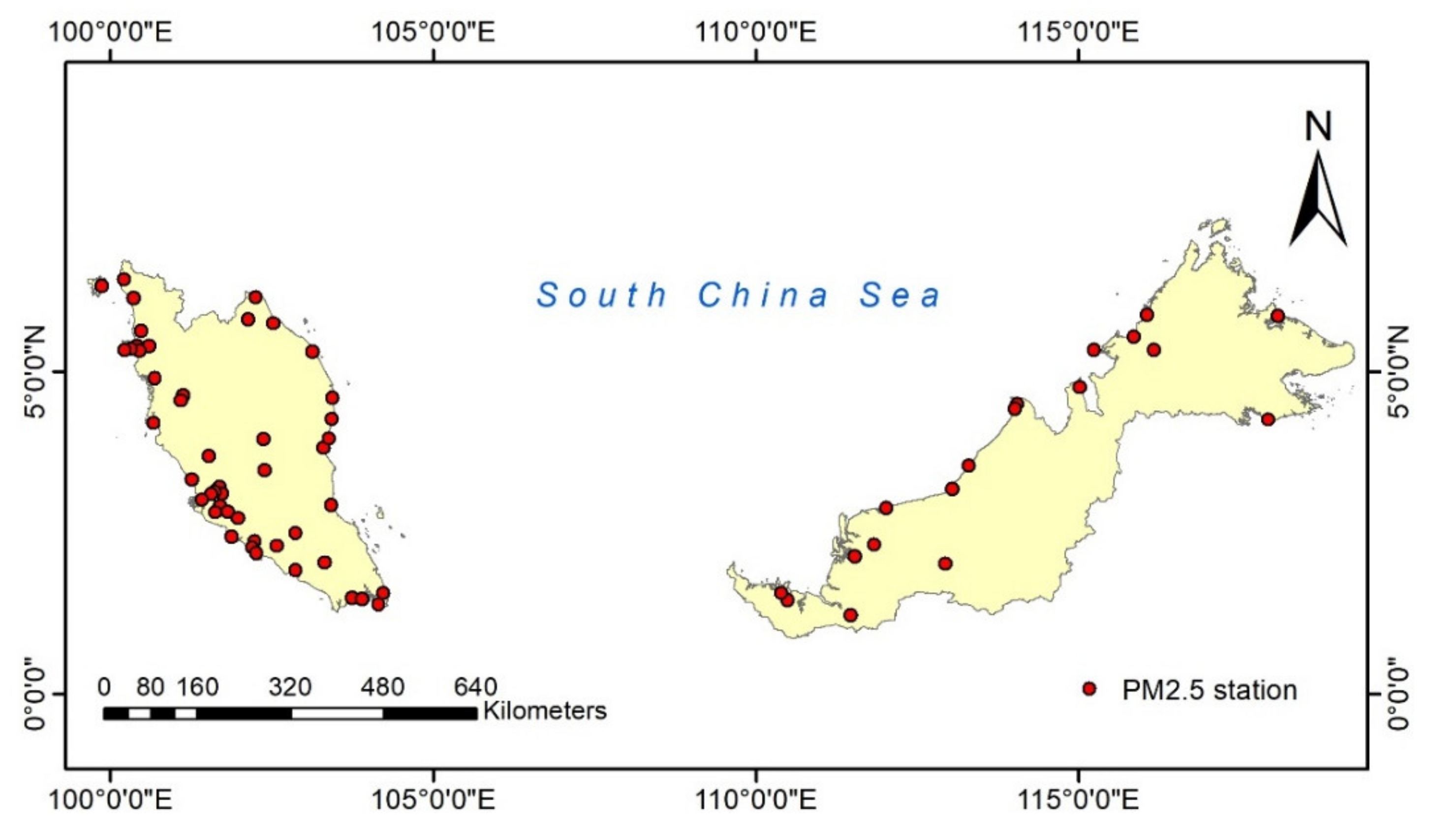
2. Study Area
3. Dataset
3.1. Ground Measurements
3.2. Satellite Data
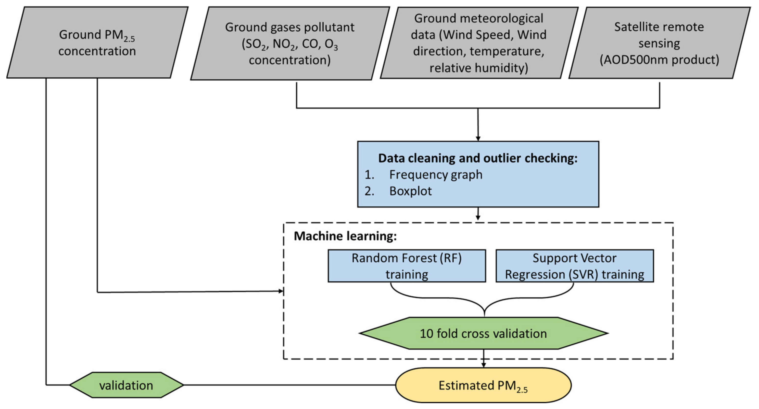
4. PM2.5 Estimation
4.1. Machine Learning (ML) for PM2.5 Estimation
4.2. Model Validation
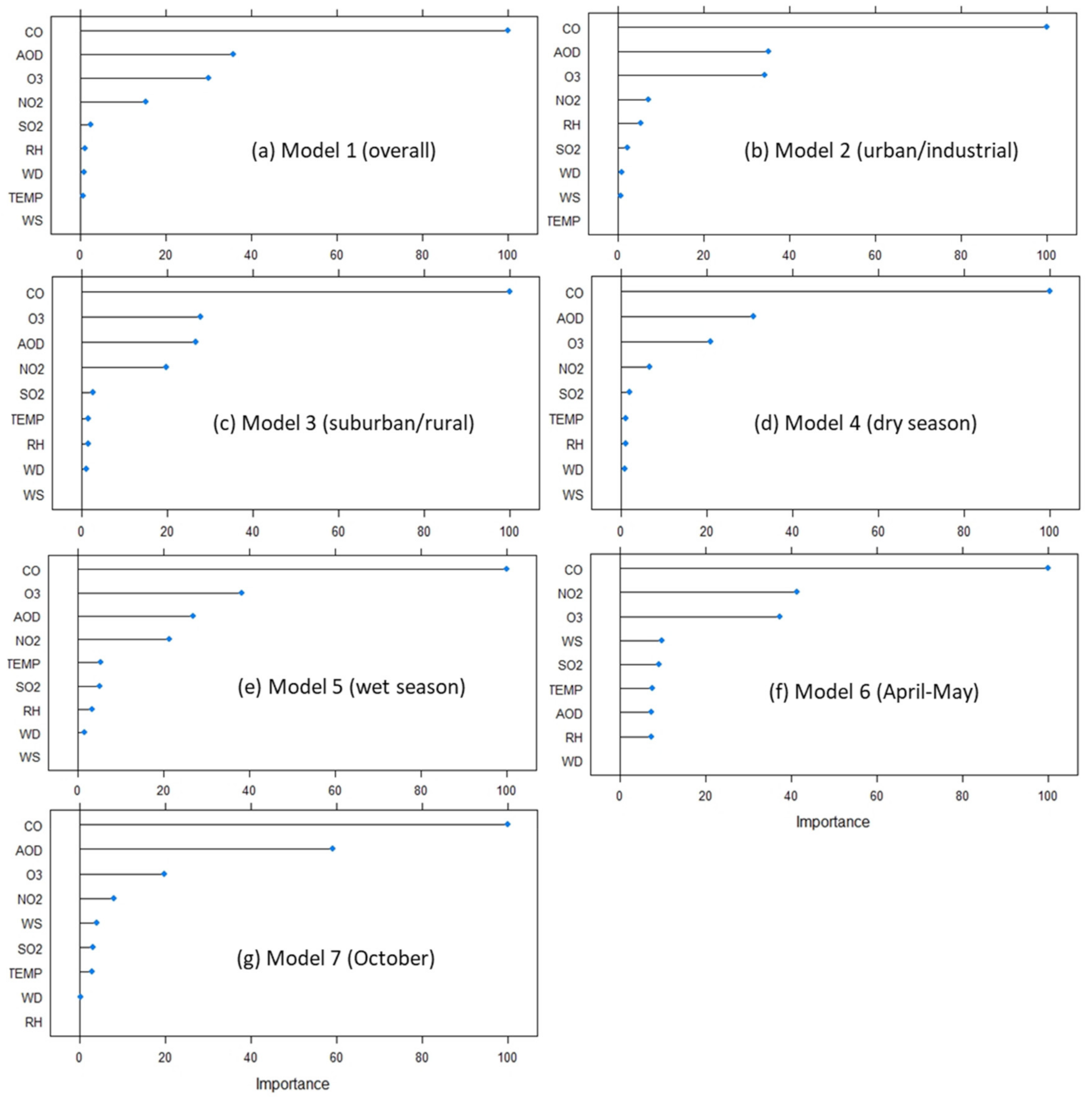
4.3. Variable Importance
5. Results and Discussion
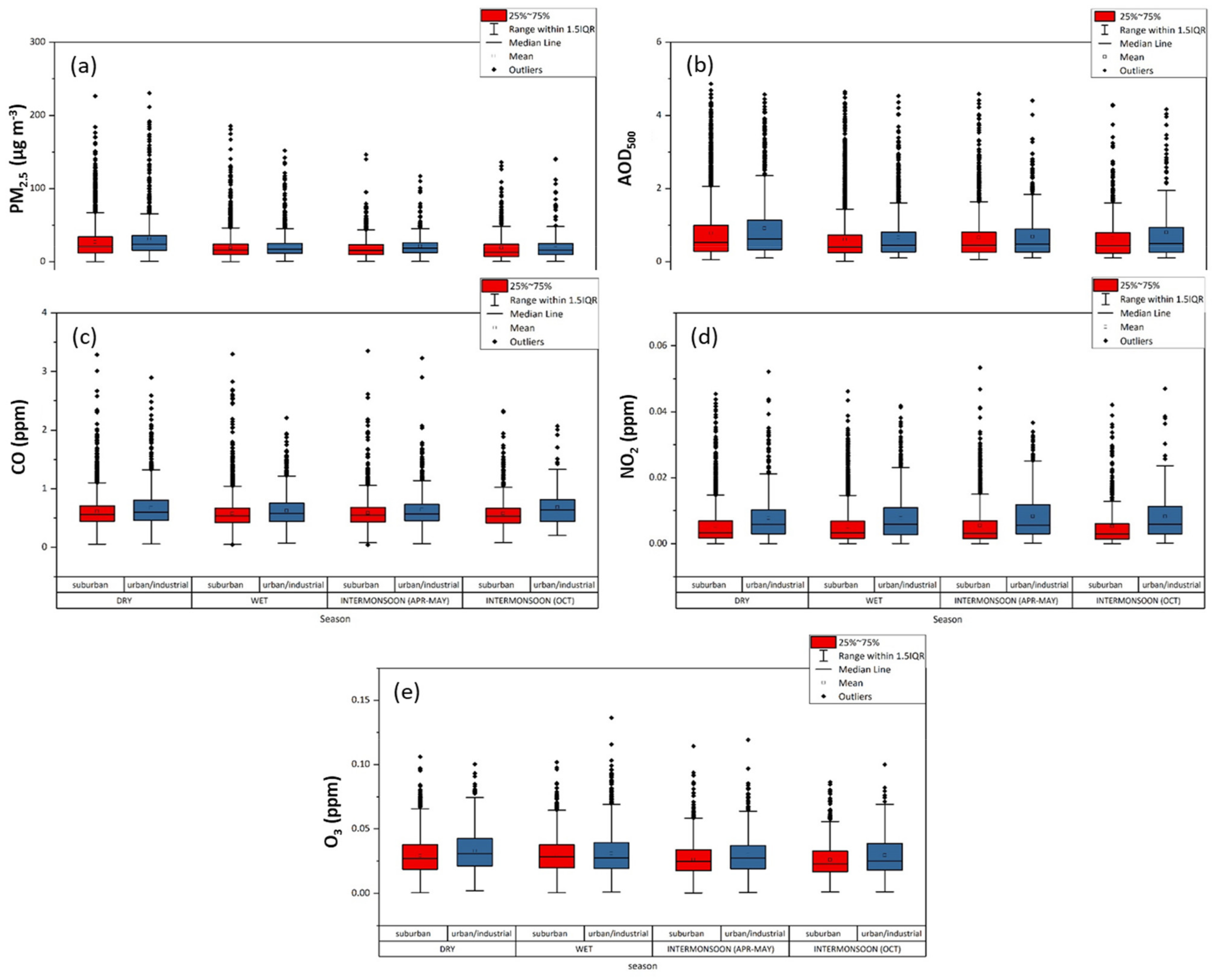
5.1. Descriptive Statistics
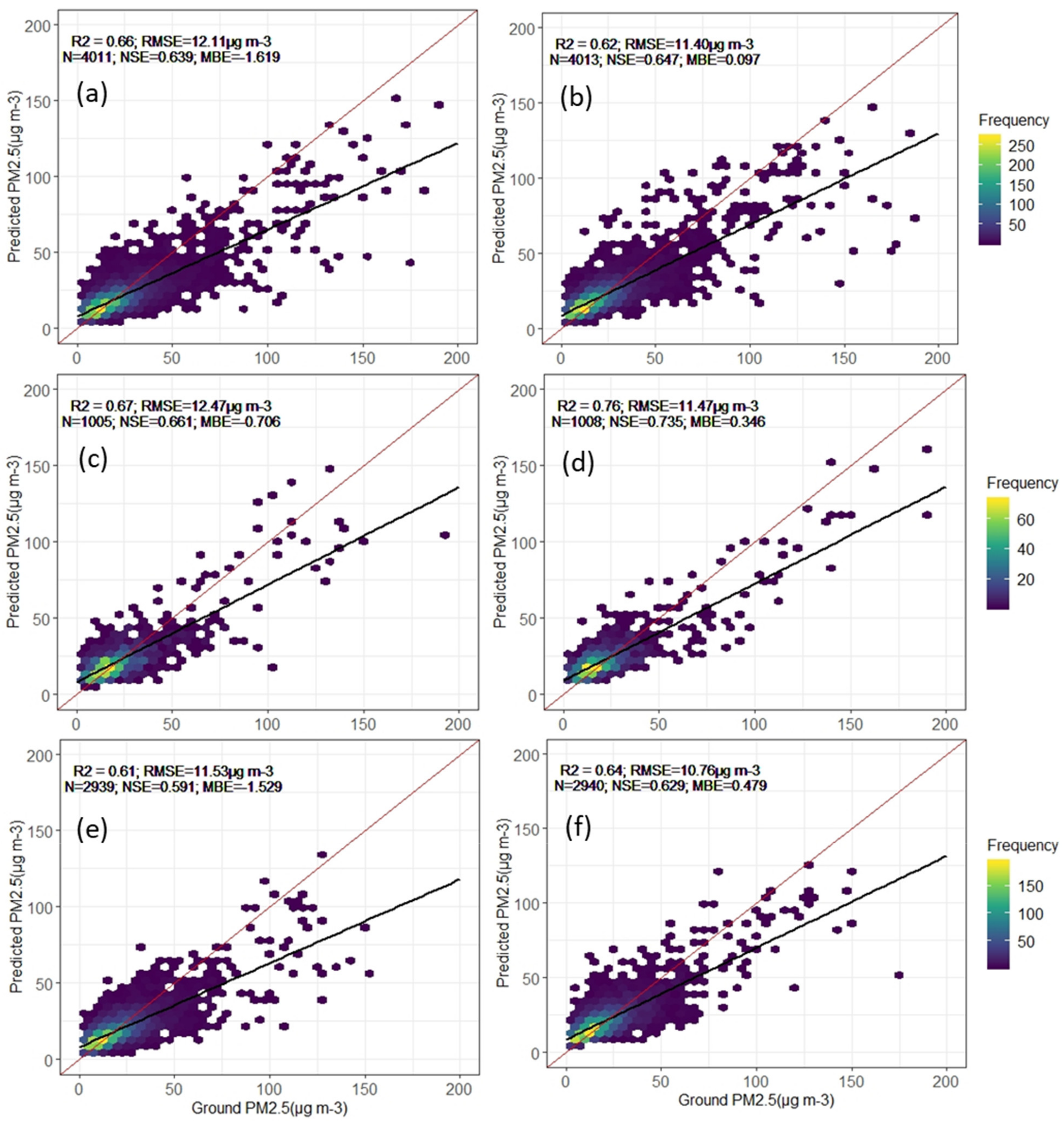
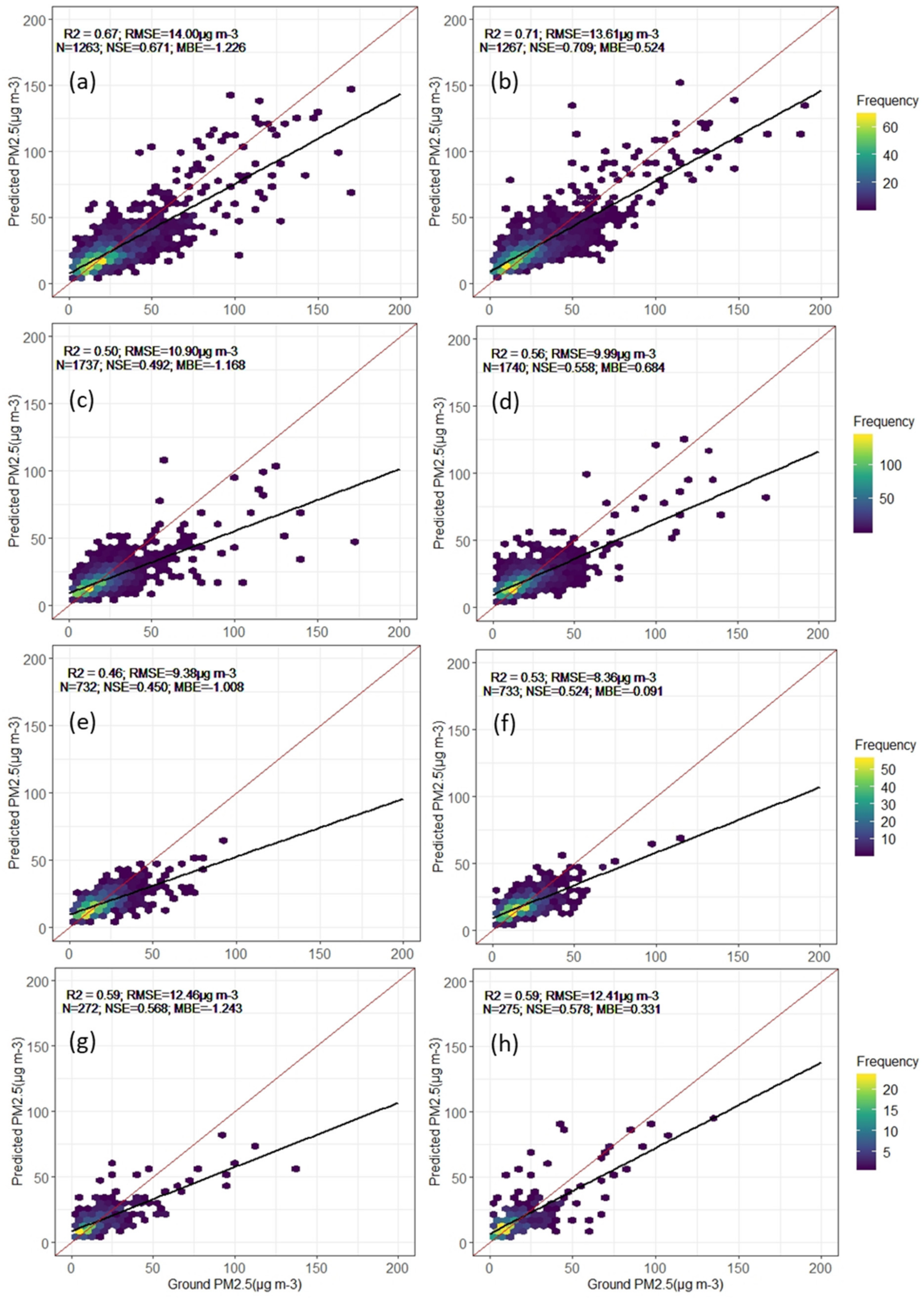
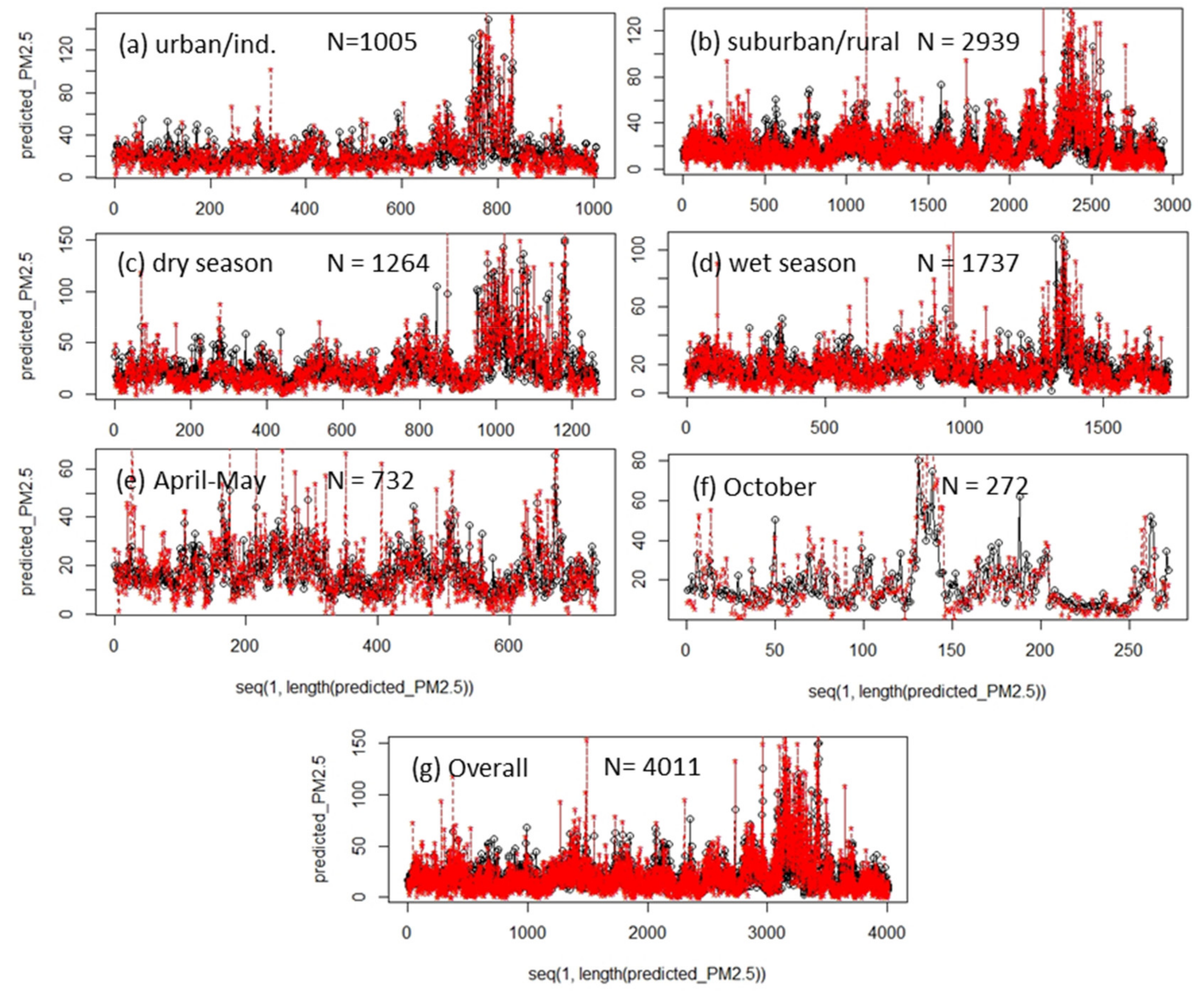
5.2. Models for PM2.5 Estimation
- Model 1: Overall model;
- Model 2: Spatial model (urban/industrial);
- Model 3: Spatial model (suburban/rural);
- Model 4: Temporal model (dry season);
- Model 5: Temporal model (wet season);
- Model 6: Temporal model (inter-monsoon, April–May);
- Model 7: Temporal model (inter-monsoon, October).
6. Conclusions
Supplementary Materials
Author Contributions
Funding
Institutional Review Board Statement
Informed Consent Statement
Data Availability Statement
Acknowledgments
Conflicts of Interest
References
- Ranjan, A.K.; Patra, A.K.; Gorai, A. A Review on Estimation of Particulate Matter from Satellite-Based Aerosol Optical Depth: Data, Methods, and Challenges. Asia Pac. J. Atmos. Sci. 2020, 57, 679–699. [Google Scholar] [CrossRef]
- Jain, S.; Sharma, S.K.; Vijayan, N.; Mandal, T.K. Seasonal characteristics of aerosols (PM2.5 and PM10) and their source apportionment using PMF: A four year study over Delhi. India. Environ. Pollut. 2020, 262, 114337. [Google Scholar] [CrossRef]
- Pani, S.K.; Wang, S.H.; Lin, N.H.; Chantara, S.; Lee, C.T.; Thepnuan, D. Black carbon over an urban atmosphere in northern peninsular Southeast Asia: Characteristics, source apportionment, and associated health risks. Environ. Pollut. 2020, 259, 113871. [Google Scholar] [CrossRef]
- WHO. WHO Global Ambient Air Quality Database. 2020. Available online: https://www.who.int/data/gho/data (accessed on 21 October 2020).
- Latif, M.T.; Othman, M.; Idris, N.; Juneng, L.; Abdullah, A.M.; Hamzah, W.P.; Khan, M.F.; Nik Sulaiman, N.M.; Jewaratnam, J.; Aghamohammadi, N.; et al. Impact of regional haze towards air quality in Malaysia: A review. Atmos. Environ. 2018, 177, 28–44. [Google Scholar] [CrossRef]
- Jamalani, M.; Abdullah, A.; Azid, A.; Ramli, M.; Baharudin, M.; Chng, L.; Elhadi, R.; Yusof, K.K.; Gnadimzadeh, A. PM 10 emission inventory of industrial and road transport vehicles in Klang Valley, Peninsular Malaysia. J. Fundam. Appl. Sci. 2018, 10, 313–324. [Google Scholar]
- Chang, S.-C. Atmospheric impacts of Indonesian fire emissions: Assessing remote sensing data and air quality during 2013 Malaysian haze. Procedia Environ. Sci. 2016, 36, 176–179. [Google Scholar]
- Gautam, R.; Hsu, N.C.; Eck, T.F.; Holben, B.N.; Janjai, S.; Jantarach, T.; Tsay, S.-C.; Lau, W.K. Characterization of aerosols over the Indochina peninsula from satellite-surface observations during biomass burning pre-monsoon season. Atmos. Environ. 2013, 78, 51–59. [Google Scholar] [CrossRef]
- Wang, S.-H.; Welton, E.J.; Holben, B.N.; Tsay, S.-C.; Lin, N.-H.; Giles, D.; Stewart, S.A.; Janjai, S.; Nguyen, X.A.; Hsiao, T.-C. Vertical distribution and columnar optical properties of springtime biomass-burning aerosols over Northern Indochina during 2014 7-SEAS campaign. Aerosol Air Qual. Res. 2015, 15, 2037–2050. [Google Scholar] [CrossRef] [Green Version]
- Reid, J.S.; Hyer, E.J.; Johnson, R.S.; Holben, B.N.; Yokelson, R.J.; Zhang, J.; Campbell, J.R.; Christopher, S.A.; Di Girolamo, L.; Giglio, L. Observing and understanding the Southeast Asian aerosol system by remote sensing: An initial review and analysis for the Seven Southeast Asian Studies (7SEAS) program. Atmos. Res. 2013, 122, 403–468. [Google Scholar] [CrossRef] [Green Version]
- Official Portal of Department of Environment. Environmental Quality Report 2019; DOE: Putrajaya, Malaysia, 2019.
- Hyer, E.J.; Reid, J.S.; Prins, E.M.; Hoffman, J.P.; Schmidt, C.C.; Miettinen, J.I.; Giglio, L. Patterns of fire activity over Indonesia and Malaysia from polar and geostationary satellite observations. Atmos. Res. 2013, 122, 504–519. [Google Scholar] [CrossRef]
- Khan, F.; Latif, M.T.; Juneng, L.; Amil, N.; Mohd Nadzir, M.S.; Syedul Hoque, H.M. Physicochemical factors and sources of particulate matter at residential urban environment in Kuala Lumpur. J. Air Waste Manag. Assoc. 2015, 65, 958–969. [Google Scholar] [CrossRef] [Green Version]
- Kanniah, K.D.; Zaman, N.A.F.K. Remotely sensed particulate matter estimation in malaysia during the biomass burning season in southeast Asia. In Biomass Burning in South and Southeast Asia Impacts on the Biosphere; Vadrevu, K.P., Ohara, T., Justice, C., Eds.; CRC Press Taylor and Francis: London, UK, 2021; Volume 2. [Google Scholar]
- Department of Statistics Malaysia, Official Portal. Statistics on Causes of Death, Malaysia, 2019. Available online: https://www.dosm.gov.my (accessed on 16 December 2020).
- Dominici, F.; Peng, R.D.; Bell, M.L.; Pham, L.; McDermott, A.; Zeger, S.L.; Samet, J.M. Fine particulate air pollution and hospital admission for cardiovascular and respiratory diseases. JAMA 2006, 295, 1127–1134. [Google Scholar] [CrossRef] [PubMed] [Green Version]
- Lary, D.; Lary, T.; Sattler, B. Using machine learning to estimate global PM2.5 for environmental health studies. Environ. Health Insights 2015, 9, EHI-S15664. [Google Scholar] [CrossRef] [PubMed]
- Zaman, N.A.; Kanniah, K.D.; Kaskaoutis, D.G. Estimating Particulate Matter using satellite based aerosol optical depth and meteorological variables in Malaysia. Atmos. Res. 2017, 193, 142–162. [Google Scholar] [CrossRef] [Green Version]
- Othman, M.; Latif, M.T.; Jamhari, A.A.; Abd Hamid, H.H.; Uning, R.; Khan, M.F.; Nadzir, M.S.M.; Sahani, M.; Wahab, M.I.A.; Chan, K.M. Spatial distribution of fine and coarse particulate matter during a southwest monsoon in Peninsular Malaysia. Chemosphere 2021, 262, 127767. [Google Scholar] [CrossRef]
- Stowe, L.L.; Ignatov, A.M.; Singh, R.R. Development, validation, and potential enhancements to the second-generation operational aerosol product at the National Environmental Satellite, Data, and Information Service of the National Oceanic and Atmospheric Administration. J. Geophys. Res. Atmos. 1997, 102, 16923–16934. [Google Scholar] [CrossRef] [Green Version]
- Ignatov, A.; Sapper, J.; Cox, S.; Laszlo, I.; Nalli, N.R.; Kidwell, K.B. Operational Aerosol Observations (AEROBS) from AVHRR/3 On Board NOAA-KLM Satellites. J. Atmos. Ocean. Technol. 2004, 21, 3–26. [Google Scholar] [CrossRef]
- Kahn, R.; Gaitley, B.; Martonchik, J.; Diner, D.; Crean, K.; Holben, B. MISR global aerosol optical depth validation based on two years of coincident data AERONET observations. J. Geophys. Res. 2004, 109. [Google Scholar] [CrossRef] [Green Version]
- Vidot, J.; Santer, R.; Aznay, O. Evaluation of the MERIS aerosol product over land with AERONET. Atmos. Chem. Phys. 2008, 8, 7603–7617. [Google Scholar] [CrossRef] [Green Version]
- Schmid, J. The SEVIRI Instrument. In Proceedings of the 2000 EUMETSAT Meteorological Satellite Data User’s Conference, Bologna, Italy, 29 May–2 June 2000. [Google Scholar]
- Remer, L.A.; Kaufman, Y.; Tanré, D.; Mattoo, S.; Chu, D.; Martins, J.V.; Li, R.-R.; Ichoku, C.; Levy, R.; Kleidman, R. The MODIS aerosol algorithm, products, and validation. J. Atmos. Sci. 2005, 62, 947–973. [Google Scholar] [CrossRef] [Green Version]
- Levy, R.; Remer, L.; Kleidman, R.; Mattoo, S.; Ichoku, C.; Kahn, R.; Eck, T. Global evaluation of the Collection 5 MODIS dark-target aerosol products over land. Atmos. Chem. Phys. 2010, 10, 10399–10420. [Google Scholar] [CrossRef] [Green Version]
- Munchak, L.; Levy, R.; Mattoo, S.; Remer, L.; Holben, B.; Schafer, J.; Hostetler, C.; Ferrare, R. MODIS 3 km aerosol product: Applications over land in an urban/suburban region. Atmos. Meas. Tech. 2013, 6, 1747–1759. [Google Scholar] [CrossRef] [Green Version]
- Sever, L.; Alpert, P.; Lyapustin, A.; Wang, Y.; Chudnovsky, A. An example of aerosol pattern variability over bright surface using high resolution MODIS MAIAC: The eastern and western areas of the Dead Sea and environs. Atmos. Environ. 2017, 165, 359–369. [Google Scholar] [CrossRef]
- Remer, L.; Mattoo, S.; Levy, R.; Munchak, L. MODIS 3km aerosol product: Algorithm and global perspective. Atmos. Meas. Tech. 2013, 6, 1829–1844. [Google Scholar] [CrossRef] [Green Version]
- Kanniah, K.D.; Kaskaoutis, D.G.; San Lim, H.; Latif, M.T.; Kamarul Zaman, N.A.F.; Liew, J. Overview of atmospheric aerosol studies in Malaysia: Known and unknown. Atmos. Res. 2016, 182, 302–318. [Google Scholar] [CrossRef]
- Zaman, N.A.; Kanniah, K.D.; Kaskaoutis, D.G. Satellite Data for Upscalling Urban Air Pollution in Malaysia. In Proceedings of the IOP Conference Series: Earth and Environmental Science, Kuala Lumpur, Malaysia, 24–25 April 2018; p. 012036. [Google Scholar]
- Kanniah, K.D.; Lim, H.Q.; Kaskaoutis, D.G.; Cracknell, A.P. Investigating aerosol properties in Peninsular Malaysia via the synergy of satellite remote sensing and ground-based measurements. Atmos. Res. 2014, 138, 223–239. [Google Scholar] [CrossRef]
- Chudnovsky, A.A.; Lee, H.J.; Kostinski, A.; Kotlov, T.; Koutrakis, P. Prediction of daily fine particulate matter concentrations using aerosol optical depth retrievals from the Geostationary Operational Environmental Satellite (GOES). J. Air Waste Manag. Assoc. 2012, 62, 1022–1031. [Google Scholar] [CrossRef]
- Xiao, Q.; Zhang, H.; Choi, M.; Li, S.; Kondragunta, S.; Kim, J.; Holben, B.; Levy, R.; Liu, Y. Evaluation of VIIRS, GOCI, and MODIS Collection 6 AOD retrievals against ground sunphotometer observations over East Asia. Atmos. Chem. Phys. 2016, 16. [Google Scholar] [CrossRef] [Green Version]
- Yang, J.; Zhang, Z.; Wei, C.; Lu, F.; Guo, Q. Introducing the new generation of Chinese geostationary weather satellites, Fengyun-4. Bull. Am. Meteorol. Soc. 2017, 98, 1637–1658. [Google Scholar] [CrossRef]
- Bessho, K.; Date, K.; Hayashi, M.; Ikeda, A.; Imai, T.; Inoue, H.; Kumagai, Y.; Miyakawa, T.; Murata, H.; Ohno, T. An introduction to Himawari-8/9—Japan’s new-generation geostationary meteorological satellites. J. Meteorol. Soc. Jpn. Ser. II 2016, 94, 151–183. [Google Scholar] [CrossRef] [Green Version]
- Zhang, W.; Xu, H.; Zhang, L. Assessment of Himawari-8 AHI Aerosol Optical Depth Over Land. Remote Sens. 2019, 11, 1108. [Google Scholar] [CrossRef] [Green Version]
- Yang, X.; Zhao, C.; Luo, N.; Zhao, W.; Shi, W.; Yan, X. Evaluation and Comparison of Himawari-8 L2 V1.0, V2.1 and MODIS C6.1 aerosol products over Asia and the oceania regions. Atmos. Environ. 2020, 220, 117068. [Google Scholar] [CrossRef]
- Imani, M. Particulate matter (PM2.5 and PM10) generation map using MODIS Level-1 satellite images and deep neural network. J. Environ. Manag. 2021, 281, 111888. [Google Scholar] [CrossRef]
- Xu, X.; Zhang, C.; Liang, Y. Review of Satellite-driven Statistical Models PM2.5 Concentration Estimation with Comprehensive Information. Atmos. Environ. 2021, 256, 118302. [Google Scholar] [CrossRef]
- Wang, J.; Christopher, S.A. Intercomparison between satellite-derived aerosol optical thickness and PM2.5 mass: Implications for air quality studies. Geophys. Res. Lett. 2003, 30, 2003. [Google Scholar] [CrossRef]
- Engel-Cox, J.A.; Holloman, C.H.; Coutant, B.W.; Hoff, R.M. Qualitative and quantitative evaluation of MODIS satellite sensor data for regional and urban scale air quality. Atmos. Environ. 2004, 38, 2495–2509. [Google Scholar] [CrossRef]
- Benas, N.; Beloconi, A.; Chrysoulakis, N. Estimation of urban PM10 concentration, based on MODIS and MERIS/AATSR synergistic observations. Atmos. Environ. 2013, 79, 448–454. [Google Scholar] [CrossRef]
- Chitranshi, S.; Sharma, S.P.; Dey, S. Satellite-based estimates of outdoor particulate pollution (PM10) for Agra City in northern India. Air Qual. Atmos. Health 2015, 8, 55–65. [Google Scholar] [CrossRef]
- Gupta, P.; Christopher, S.A. Particulate matter air quality assessment using integrated surface, satellite, and meteorological products: Multiple regression approach. J. Geophys. Res. Atmos. 2009, 114. [Google Scholar] [CrossRef] [Green Version]
- Schaap, M.; Apituley, A.; Timmermans, R.; Koelemeijer, R.; Leeuw, G.D. Exploring the relation between aerosol optical depth and PM 2.5 at Cabauw, the Netherlands. Atmos. Chem. Phys. 2009, 9, 909–925. [Google Scholar] [CrossRef] [Green Version]
- Liu, Y.; Park, R.J.; Jacob, D.J.; Li, Q.; Kilaru, V.; Sarnat, J.A. Mapping annual mean ground-level PM2.5 concentrations using Multiangle Imaging Spectroradiometer aerosol optical thickness over the contiguous United States. J. Geophys. Res. Atmos. 2004, 109. [Google Scholar] [CrossRef]
- Van Donkelaar, A.; Martin, R.V.; Park, R.J. Estimating ground-level PM2.5 using aerosol optical depth determined from satellite remote sensing. J. Geophys. Res. Atmos. 2006, 111. [Google Scholar] [CrossRef]
- Engel-Cox, J.; Oanh, N.T.; van Donkelaar, A.; Martin, R.V.; Zell, E. Toward the next generation of air quality monitoring: Particulate Matter. Atmos. Environ. 2013, 80, 584–590. [Google Scholar] [CrossRef]
- Crouse, D.L.; Philip, S.; Van Donkelaar, A.; Martin, R.V.; Jessiman, B.; Peters, P.A.; Weichenthal, S.; Brook, J.R.; Hubbell, B.; Burnett, R.T. A new method to jointly estimate the mortality risk of long-term exposure to fine particulate matter and its components. Sci. Rep. 2016, 6, 18916. [Google Scholar] [CrossRef] [PubMed] [Green Version]
- Lee, H.; Liu, Y.; Coull, B.; Schwartz, J.; Koutrakis, P. A novel calibration approach of MODIS AOD data to predict PM 2.5 concentrations. Atmos. Chem. Phys. Discuss. 2011, 11, 7991–8002. [Google Scholar] [CrossRef] [Green Version]
- Kloog, I.; Koutrakis, P.; Coull, B.A.; Lee, H.J.; Schwartz, J. Assessing temporally and spatially resolved PM2.5 exposures for epidemiological studies using satellite aerosol optical depth measurements. Atmos. Environ. 2011, 45, 6267–6275. [Google Scholar] [CrossRef]
- Xie, Y.; Wang, Y.; Zhang, K.; Dong, W.; Lv, B.; Bai, Y. Daily estimation of ground-level PM2.5 concentrations over Beijing using 3 km resolution MODIS AOD. Environ. Sci. Technol. 2015, 49, 12280–12288. [Google Scholar] [CrossRef] [Green Version]
- Beloconi, A.; Kamarianakis, Y.; Chrysoulakis, N. Estimating urban PM10 and PM2.5 concentrations, based on synergistic MERIS/AATSR aerosol observations, land cover and morphology data. Remote Sens. Environ. 2016, 172, 148–164. [Google Scholar] [CrossRef] [Green Version]
- Gupta, P.; Christopher, S.A. Particulate matter air quality assessment using integrated surface, satellite, and meteorological products: 2. A neural network approach. J. Geophys. Res. Atmos. 2009, 114. [Google Scholar] [CrossRef]
- Di, Q.; Kloog, I.; Koutrakis, P.; Lyapustin, A.; Wang, Y.; Schwartz, J. Assessing PM2.5 exposures with high spatiotemporal resolution across the continental United States. Environ. Sci. Technol. 2016, 50, 4712–4721. [Google Scholar] [CrossRef] [Green Version]
- Wu, Y.; Guo, J.; Zhang, X.; Li, X. Correlation between PM Concentrations and Aerosol Optical Depth in Eastern China Based on BP Neural Networks. In Proceedings of the Geoscience and Remote Sensing Symposium (IGARSS), 2011 IEEE International, Vancouver, BC, Canada, 24–29 July 2011; pp. 3308–3311. [Google Scholar]
- Grivas, G.; Chaloulakou, A. Artificial neural network models for prediction of PM10 hourly concentrations, in the Greater Area of Athens, Greece. Atmos. Environ. 2006, 40, 1216–1229. [Google Scholar] [CrossRef]
- Hu, Z. Spatial analysis of MODIS aerosol optical depth, PM 2.5, and chronic coronary heart disease. Int. J. Health Geogr. 2009, 8, 27. [Google Scholar] [CrossRef] [PubMed] [Green Version]
- Ma, Z.; Hu, X.; Huang, L.; Bi, J.; Liu, Y. Estimating ground-level PM2.5 in China using satellite remote sensing. Environ. Sci. Technol. 2014, 48, 7436–7444. [Google Scholar] [CrossRef]
- You, W.; Zang, Z.; Zhang, L.; Li, Y.; Pan, X.; Wang, W. National-scale estimates of ground-level PM2.5 concentration in China using geographically weighted regression based on 3 km resolution MODIS AOD. Remote Sens. 2016, 8, 184. [Google Scholar] [CrossRef] [Green Version]
- Bai, Y.; Wu, L.; Qin, K.; Zhang, Y.; Shen, Y.; Zhou, Y. A geographically and temporally weighted regression model for ground-level PM2.5 estimation from satellite-derived 500 m resolution AOD. Remote Sens. 2016, 8, 262. [Google Scholar] [CrossRef] [Green Version]
- Paciorek, C.J.; Liu, Y.; Moreno-Macias, H.; Kondragunta, S. Spatiotemporal associations between GOES aerosol optical depth retrievals and ground-level PM2.5. Environ. Sci. Technol. 2008, 42, 5800–5806. [Google Scholar] [CrossRef] [Green Version]
- Liu, Y.; Paciorek, C.J.; Koutrakis, P. Estimating regional spatial and temporal variability of PM2.5 concentrations using satellite data, meteorology, and land use information. Environ. Health Perspect. 2009, 117, 886. [Google Scholar] [CrossRef] [Green Version]
- Song, Y.-Z.; Yang, H.-L.; Peng, J.-H.; Song, Y.-R.; Sun, Q.; Li, Y. Estimating PM2.5 concentrations in Xi’an City using a generalized additive model with multi-source monitoring data. PLoS ONE 2015, 10, e0142149. [Google Scholar] [CrossRef] [PubMed] [Green Version]
- Zou, B.; Chen, J.; Zhai, L.; Fang, X.; Zheng, Z. Satellite based mapping of ground PM2.5 concentration using generalized additive modeling. Remote Sens. 2016, 9, 1. [Google Scholar] [CrossRef] [Green Version]
- Hu, X.; Waller, L.A.; Lyapustin, A.; Wang, Y.; Al-Hamdan, M.Z.; Crosson, W.L.; Estes Jr, M.G.; Estes, S.M.; Quattrochi, D.A.; Puttaswamy, S.J. Estimating ground-level PM2.5 concentrations in the Southeastern United States using MAIAC AOD retrievals and a two-stage model. Remote Sens. Environ. 2014, 140, 220–232. [Google Scholar] [CrossRef]
- Ma, Z.; Hu, X.; Sayer, A.M.; Levy, R.; Zhang, Q.; Xue, Y.; Tong, S.; Bi, J.; Huang, L.; Liu, Y. Satellite-based spatiotemporal trends in PM2.5 concentrations: China, 2004–2013. Environ. Health Perspect. 2016, 124, 184. [Google Scholar] [CrossRef] [Green Version]
- Li, L.; Chen, B.; Zhang, Y.; Zhao, Y.; Xian, Y.; Xu, G.; Zhang, H.; Guo, L. Retrieval of Daily PM2.5 Concentrations Using Nonlinear Methods: A Case Study of the Beijing–Tianjin–Hebei Region, China. Remote Sens. 2018, 10, 2006. [Google Scholar] [CrossRef] [Green Version]
- Danesh Yazdi, M.; Kuang, Z.; Dimakopoulou, K.; Barratt, B.; Suel, E.; Amini, H.; Lyapustin, A.; Katsouyanni, K.; Schwartz, J. Predicting Fine Particulate Matter (PM2.5) in the Greater London Area: An Ensemble Approach using Machine Learning Methods. Remote Sens. 2020, 12, 914. [Google Scholar] [CrossRef] [Green Version]
- Kleine Deters, J.; Zalakeviciute, R.; Gonzalez, M.; Rybarczyk, Y. Modeling PM2.5 urban pollution using machine learning and selected meteorological parameters. J. Electr. Comput. Eng. 2017, 2017. [Google Scholar] [CrossRef] [Green Version]
- Shin, M.; Kang, Y.; Park, S.; Im, J.; Yoo, C.; Quackenbush, L.J. Estimating ground-level particulate matter concentrations using satellite-based data: A review. GIScience Remote Sens. 2020, 57, 174–189. [Google Scholar] [CrossRef]
- Gholami, H.; Mohamadifar, A.; Sorooshian, A.; Jansen, J.D. Machine-learning algorithms for predicting land susceptibility to dust emissions: The case of the Jazmurian Basin, Iran. Atmos. Pollut. Res. 2020, 11, 1303–1315. [Google Scholar] [CrossRef]
- Gholami, H.; Mohammadifar, A.; Bui, D.T.; Collins, A.L. Mapping wind erosion hazard with regression-based machine learning algorithms. Sci. Rep. 2020, 10, 1–16. [Google Scholar] [CrossRef] [PubMed]
- Guo, Y.; Tang, Q.; Gong, D.-Y.; Zhang, Z. Estimating ground-level PM2.5 concentrations in Beijing using a satellite-based geographically and temporally weighted regression model. Remote Sens. Environ. 2017, 198, 140–149. [Google Scholar] [CrossRef]
- Hu, X.; Waller, L.A.; Al-Hamdan, M.Z.; Crosson, W.L.; Estes Jr, M.G.; Estes, S.M.; Quattrochi, D.A.; Sarnat, J.A.; Liu, Y. Estimating ground-level PM2.5 concentrations in the southeastern US using geographically weighted regression. Environ. Res. 2013, 121, 1–10. [Google Scholar] [CrossRef]
- Jiang, M.; Sun, W.; Yang, G.; Zhang, D. Modelling seasonal GWR of daily PM2.5 with proper auxiliary variables for the Yangtze River Delta. Remote Sens. 2017, 9, 346. [Google Scholar] [CrossRef] [Green Version]
- Luo, J.; Du, P.; Samat, A.; Xia, J.; Che, M.; Xue, Z. Spatiotemporal pattern of PM 2.5 concentrations in mainland China and analysis of its influencing factors using geographically weighted regression. Sci. Rep. 2017, 7, 1–14. [Google Scholar]
- Gholami, H.; Kordestani, M.D.; Li, J.; Telfer, M.W.; Fathabadi, A. Diverse sources of aeolian sediment revealed in an arid landscape in southeastern Iran using a modified Bayesian un-mixing model. Aeolian Res. 2019, 41, 100547. [Google Scholar] [CrossRef]
- Kusuma, W.L.; Chih-Da, W.; Yu-Ting, Z.; Hapsari, H.H.; Muhamad, J.L. PM2.5 pollutant in Asia—a comparison of metropolis cities in Indonesia and Taiwan. Int. J. Environ. Res. Public Health 2019, 16, 4924. [Google Scholar] [CrossRef] [PubMed] [Green Version]
- Amil, N.; Latif, M.T.; Khan, M.F.; Mohamad, M. Seasonal variability of PM 2.5 composition and sources in the Klang Valley urban-industrial environment. Atmos. Chem. Phys. 2016, 16, 5357–5381. [Google Scholar] [CrossRef] [Green Version]
- Grange, S.K.; Carslaw, D.C.; Lewis, A.C.; Boleti, E.; Hueglin, C. Random forest meteorological normalisation models for Swiss PM 10 trend analysis. Atmos. Chem. Phys. 2018, 18, 6223–6239. [Google Scholar] [CrossRef] [Green Version]
- Lovrić, M.; Pavlović, K.; Vuković, M.; Grange, S.K.; Haberl, M.; Kern, R. Understanding the true effects of the COVID-19 lockdown on air pollution by means of machine learning. Environ. Pollut. 2021, 274, 115900. [Google Scholar] [CrossRef]
- Šimić, I.; Lovrić, M.; Godec, R.; Kröll, M.; Bešlić, I. Applying machine learning methods to better understand, model and estimate mass concentrations of traffic-related pollutants at a typical street canyon. Environ. Pollut. 2020, 263, 114587. [Google Scholar] [CrossRef]
- Shaziayani, W.N.; Ul-Saufie, A.Z.; Libasin, Z.; Shukri, F.N.A.; Abdullah, S.S.S.; Noor, N.M. A Review of PM10 Concentrations Modelling in Malaysia. In Proceedings of the IOP Conference Series: Earth and Environmental Science, Seoul, Korea, 23–24 July 2020; p. 12008. [Google Scholar]
- Dahari, N.; Latif, M.T.; Muda, K.; Hussein, N. Influence of Meteorological Variables on Suburban Atmospheric PM2.5 in the Southern Region of Peninsular Malaysia. Aerosol Air Qual. Res. 2020, 20, 14–25. [Google Scholar] [CrossRef]
- Ee-Ling, O.; Mustaffa, N.I.H.; Amil, N.; Khan, M.F.; Latif, M.T. Source contribution of PM 2.5 at different locations on the Malaysian Peninsula. Bull. Environ. Contam. Toxicol. 2015, 94, 537–542. [Google Scholar] [CrossRef] [PubMed]
- Yaakob, U.; Masron, T.; Masami, F. Ninety years of urbanization in Malaysia: A geographical investigation of its trends and characteristics. J. Ritsumeikan Soc. Sci Hum. 2010, 4, 79–101. [Google Scholar]
- Jamil, A.; Makmom, A.A.; Saeid, P.; Firuz, R.M.; Prinaz, R. PM10 monitoring using MODIS AOT and GIS, Kuala Lumpur, Malaysia. Res. J. Chem. Environ. 2011, 15, 2. [Google Scholar]
- Abas, M.R.; Oros, D.R.; Simoneit, B.R. Biomass burning as the main source of organic aerosol particulate matter in Malaysia during haze episodes. Chemosphere 2004, 55, 1089–1095. [Google Scholar] [CrossRef] [PubMed]
- Awang, M.B.; Jaafar, A.B.; Abdullah, A.M.; Ismail, M.B.; Hassan, M.N.; Abdullah, R.; Johan, S.; Noor, H. Air quality in Malaysia: Impacts, management issues and future challenges. Respirology 2000, 5, 183–196. [Google Scholar] [CrossRef]
- Kanniah, K.D.; Zaman, N.A.F.K.; Kaskaoutis, D.G.; Latif, M.T. COVID-19’s impact on the atmospheric environment in the Southeast Asia region. Sci. Total Environ. 2020, 736, 139658. [Google Scholar] [CrossRef] [PubMed]
- Ash’aari, Z.H.; Aris, A.Z.; Ezani, E.; Kamal, N.I.A.; Jaafar, N.; Jahaya, J.N.; Manan, S.A.; Saifuddin, M.F.U. Spatiotemporal variations and contributing factors of air pollutant concentrations in Malaysia during movement control order due to pandemic COVID-19. Aerosol Air Qual. Res. 2020, 20, 2047–2061. [Google Scholar] [CrossRef]
- Alhasa, K.M.; Mohd Nadzir, M.S.; Olalekan, P.; Latif, M.T.; Yusup, Y.; Iqbal Faruque, M.R.; Ahamad, F.; Aiyub, K.; Md Ali, S.H.; Khan, M.F. Calibration model of a low-cost air quality sensor using an adaptive neuro-fuzzy inference system. Sensors 2018, 18, 4380. [Google Scholar] [CrossRef] [Green Version]
- Latif, M.T.; Dominick, D.; Hawari, N.S.S.L.; Mohtar, A.A.A.; Othman, M. The concentration of major air pollutants during the movement control order due to the COVID-19 pandemic in the Klang Valley, Malaysia. Sustain. Cities Soc. 2021, 66, 102660. [Google Scholar] [CrossRef]
- Li, T.; Zhang, C.; Shen, H.; Yuan, Q.; Zhang, L. Real-time and Seamless Monitoring of Ground-Level PM2.5 Using Satellite Remote Sensing. arXiv 2018, arXiv:1803.03409. [Google Scholar]
- Sowden, M.; Mueller, U.; Blake, D. Review of surface particulate monitoring of dust events using geostationary satellite remote sensing. Atmos. Environ. 2018, 183, 154–164. [Google Scholar] [CrossRef]
- Liu, J.; Weng, F.; Li, Z.; Cribb, M.C. Hourly PM2.5 Estimates from a Geostationary Satellite Based on an Ensemble Learning Algorithm and Their Spatiotemporal Patterns over Central East China. Remote Sens. 2019, 11, 2120. [Google Scholar] [CrossRef] [Green Version]
- Zang, L.; Mao, F.; Guo, J.; Gong, W.; Wang, W.; Pan, Z. Estimating hourly PM1 concentrations from Himawari-8 aerosol optical depth in China. Environ. Pollut. 2018, 241, 654–663. [Google Scholar] [CrossRef] [PubMed]
- She, L.; Xue, Y.; Yang, X.; Guang, J.; Li, Y.; Che, Y.; Fan, C.; Xie, Y. Dust detection and intensity estimation using Himawari-8/AHI observation. Remote Sens. 2018, 10, 490. [Google Scholar] [CrossRef] [Green Version]
- Yumimoto, K.; Nagao, T.; Kikuchi, M.; Sekiyama, T.; Murakami, H.; Tanaka, T.; Ogi, A.; Irie, H.; Khatri, P.; Okumura, H. Aerosol data assimilation using data from Himawari-8, a next-generation geostationary meteorological satellite. Geophys. Res. Lett. 2016, 43, 5886–5894. [Google Scholar] [CrossRef]
- Kikuchi, M.; Murakami, H.; Suzuki, K.; Nagao, T.M.; Higurashi, A. Improved hourly estimates of aerosol optical thickness using spatiotemporal variability derived from Himawari-8 geostationary satellite. IEEE Trans. Geosci. Remote Sens. 2018, 56, 3442–3455. [Google Scholar] [CrossRef]
- Chen, J.; Huang, X. Estimating Hourly PM 2.5 Concentrations from Himawari-8 AOD over Hubei Province. Int. Arch. Photogramm. Remote Sens. Spat. Inf. Sci. 2018, 42. [Google Scholar] [CrossRef]
- Zaman, N.A.F.K.; Kanniah, K.D. Spatio-temporal assessment of Aerosol Optical Depth from Himawari-8 Satellite Data over Malaysia. In Proceedings of the IOP Conference Series: Earth and Environmental Science, Kuala Lumpur, Malaysia, 20–21 October 2020; p. 12053. [Google Scholar]
- Wei, H.; Wang, W.; Xu, F.; Feng, J. Evaluation of the Himawari-8 Aerosol Products. In Proceedings of the IGARSS 2019—2019 IEEE International Geoscience and Remote Sensing Symposium, Yokohama, Japan, 28 July–2 August 2019; pp. 7825–7828. [Google Scholar]
- Choi, M.; Lim, H.; Kim, J.; Lee, S.; Eck, T.F.; Holben, B.N.; Garay, M.J.; Hyer, E.J.; Saide, P.E.; Liu, H. Validation, comparison, and integration of GOCI, AHI, MODIS, MISR, and VIIRS aerosol optical depth over East Asia during the 2016 KORUS-AQ campaign. Meas. Tech. 2019, 12, 4619–4641. [Google Scholar] [CrossRef] [Green Version]
- Wei, J.; Li, Z.; Sun, L.; Peng, Y.; Zhang, Z.; Li, Z.; Su, T.; Feng, L.; Cai, Z.; Wu, H. Evaluation and uncertainty estimate of next-generation geostationary meteorological Himawari-8/AHI aerosol products. Sci. Total Environ. 2019, 692, 879–891. [Google Scholar] [CrossRef] [PubMed]
- Liu, B.-C.; Binaykia, A.; Chang, P.-C.; Tiwari, M.K.; Tsao, C.-C. Urban air quality forecasting based on multi-dimensional collaborative Support Vector Regression (SVR): A case study of Beijing-Tianjin-Shijiazhuang. PLoS ONE 2017, 12, e0179763. [Google Scholar] [CrossRef] [PubMed]
- Wu, C.; Wu, D.; Yu, J.Z. Estimation and uncertainty analysis of secondary organic carbon using 1 year of hourly organic and elemental carbon data. J. Geophys. Res. Atmos. 2019, 124, 2774–2795. [Google Scholar] [CrossRef]
- Su, T.; Li, Z.; Li, C.; Li, J.; Han, W.; Shen, C.; Tan, W.; Wei, J.; Guo, J. The significant impact of aerosol vertical structure on lower atmosphere stability and its critical role in aerosol–planetary boundary layer (PBL) interactions. Atmos. Chem. Phys. 2020, 20, 3713–3724. [Google Scholar] [CrossRef] [Green Version]
- Zang, L.; Wang, Z.; Zhu, B.; Zhang, Y. Roles of relative humidity in aerosol pollution aggravation over Central China during wintertime. Int. J. Environ. Res. Public Health 2019, 16, 4422. [Google Scholar] [CrossRef] [Green Version]
- Wang, J.; Martin, S.T. Satellite characterization of urban aerosols: Importance of including hygroscopicity and mixing state in the retrieval algorithms. J. Geophys. Res. Atmos. 2007, 112. [Google Scholar] [CrossRef] [Green Version]
- Titos, G.; Cazorla, A.; Zieger, P.; Andrews, E.; Lyamani, H.; Granados-Muñoz, M.J.; Olmo, F.; Alados-Arboledas, L. Effect of hygroscopic growth on the aerosol light-scattering coefficient: A review of measurements, techniques and error sources. Atmos. Environ. 2016, 141, 494–507. [Google Scholar] [CrossRef] [Green Version]
- Ul-Saufie, A.Z.; Yahaya, A.S.; Ramli, N.; Hamid, H.A. Performance of multiple linear regression model for long-term PM10 concentration prediction based on gaseous and meteorological parameters. J. Appl. Sci. 2012, 12, 1488–1494. [Google Scholar] [CrossRef]
- Abdullah, S.; Ismail, M.; Ahmed, A.N.; Abdullah, A.M. Forecasting particulate matter concentration using linear and non-linear approaches for air quality decision support. Atmosphere 2019, 10, 667. [Google Scholar] [CrossRef] [Green Version]
- Ahmad, M.; Alam, K.; Tariq, S.; Anwar, S.; Nasir, J.; Mansha, M. Estimating fine particulate concentration using a combined approach of linear regression and artificial neural network. Atmos. Environ. 2019, 219, 117050. [Google Scholar] [CrossRef]
- Stafoggia, M.; Bellander, T.; Bucci, S.; Davoli, M.; De Hoogh, K.; De’Donato, F.; Gariazzo, C.; Lyapustin, A.; Michelozzi, P.; Renzi, M. Estimation of daily PM10 and PM2.5 concentrations in Italy, 2013–2015, using a spatiotemporal land-use random-forest model. Environ. Int. 2019, 124, 170–179. [Google Scholar] [CrossRef]
- Mhawish, A.; Banerjee, T.; Sorek-Hamer, M.; Bilal, M.; Lyapustin, A.I.; Chatfield, R.; Broday, D.M. Estimation of high-resolution PM2.5 over the indo-gangetic plain by fusion of satellite data, meteorology, and land use variables. Environ. Sci. Technol. 2020, 54, 7891–7900. [Google Scholar] [CrossRef]
- Jiang, T.; Chen, B.; Nie, Z.; Ren, Z.; Xu, B.; Tang, S. Estimation of hourly full-coverage PM2.5 concentrations at 1-km resolution in China using a two-stage random forest model. Atmos. Res. 2021, 248, 105146. [Google Scholar] [CrossRef]
- Awad, M.; Khanna, R. Support Vector Regression. In Efficient Learning Machines: Theories, Concepts, and Applications for Engineers and System Designers; Apress: Berkeley, CA, USA, 2015; pp. 67–80. [Google Scholar] [CrossRef] [Green Version]
- Weizhen, H.; Zhengqiang, L.; Yuhuan, Z.; Hua, X.; Ying, Z.; Kaitao, L.; Donghui, L.; Peng, W.; Yan, M. Using Support Vector Regression to Predict PM10 and PM2.5. In Proceedings of the IOP Conference Series: Earth and Environmental Science, Beijing, China, 22–26 April 2013; p. 12268. [Google Scholar]
- Breiman, L. Random forests. Mach. Learn. 2001, 45, 5–32. [Google Scholar] [CrossRef] [Green Version]
- Sage, A. Random Forest Robustness, Variable Importance, and Tree Aggregation. 2018. Available online: https://lib.dr.iastate.edu/etd/16453 (accessed on 20 May 2021).
- Hou, N.; Zhang, X.; Zhang, W.; Wei, Y.; Jia, K.; Yao, Y.; Jiang, B.; Cheng, J. Estimation of Surface Downward Shortwave Radiation over China from Himawari-8 AHI Data Based on Random Forest. Remote Sens. 2020, 12, 181. [Google Scholar] [CrossRef] [Green Version]
- Strobl, C.; Malley, J.; Tutz, G. An introduction to recursive partitioning: Rationale, application, and characteristics of classification and regression trees, bagging, and random forests. Psychol. Methods 2009, 14, 323. [Google Scholar] [CrossRef] [Green Version]
- Janitza, S.; Hornung, R. On the overestimation of random forest’s out-of-bag error. PLoS ONE 2018, 13, e0201904. [Google Scholar] [CrossRef]
- Hu, X.; Belle, J.H.; Meng, X.; Wildani, A.; Waller, L.A.; Strickland, M.J.; Liu, Y. Estimating PM2.5 concentrations in the conterminous United States using the random forest approach. Environ. Sci. Technol. 2017, 51, 6936–6944. [Google Scholar] [CrossRef] [PubMed]
- Brokamp, C.; Jandarov, R.; Hossain, M.; Ryan, P. Predicting daily urban fine particulate matter concentrations using a random forest model. Environ. Sci. Technol. 2018, 52, 4173–4179. [Google Scholar] [CrossRef]
- Genuer, R.; Poggi, J.-M.; Tuleau-Malot, C. Variable selection using random forests. Pattern Recognit. Lett. 2010, 31, 2225–2236. [Google Scholar] [CrossRef] [Green Version]
- Li, T.; Shen, H.; Zeng, C.; Yuan, Q. A Validation approach considering the uneven distribution of ground stations for satellite-based PM 2.5 estimation. IEEE J. Sel. Top. Appl. Earth Obs. Remote Sens. 2020, 13, 1312–1321. [Google Scholar] [CrossRef]
- Strobl, C.; Boulesteix, A.-L.; Zeileis, A.; Hothorn, T. Bias in random forest variable importance measures: Illustrations, sources and a solution. BMC Bioinform. 2007, 8, 1–21. [Google Scholar] [CrossRef] [Green Version]
- Kalita, G.; Kunchala, R.K.; Fadnavis, S.; Kaskaoutis, D.G. Long term variability of carbonaceous aerosols over Southeast Asia via reanalysis: Association with changes in vegetation cover and biomass burning. Atmos. Res. 2020, 245, 105064. [Google Scholar] [CrossRef]
- Pani, S.K.; Lin, N.-H.; Griffith, S.M.; Chantara, S.; Lee, C.-T.; Thepnuan, D.; Tsai, Y.I. Brown carbon light absorption over an urban environment in northern peninsular Southeast Asia. Environ. Pollut. 2021, 276, 116735. [Google Scholar] [CrossRef]
- Nguyen, T.P.M.; Bui, T.H.; Nguyen, M.K.; Nguyen, T.H.; Pham, H.L. Impact of COVID-19 partial lockdown on PM 2.5, SO2, NO2, O3, and trace elements in PM 2.5 in Hanoi, Vietnam. Environ. Sci. Pollut. Res. 2021, 1–11. [Google Scholar] [CrossRef]
- Grivas, G.; Dimakopoulou, K.; Samoli, E.; Papakosta, D.; Karakatsani, A.; Katsouyanni, K.; Chaloulakou, A. Ozone exposure assessment for children in Greece-Results from the RESPOZE study. Sci. Total Environ. 2017, 581, 518–529. [Google Scholar] [CrossRef]
- Hatzianastassiou, N.; Katsoulis, B.D.; Antakis, B. Extreme nitrogen oxide and ozone concentrations in Athens atmosphere in relation to meteorological conditions. Environ. Monit. Assess. 2007, 128, 447–464. [Google Scholar] [CrossRef] [PubMed]
- Jin, Q.; Crippa, P.; Pryor, S. Spatial characteristics and temporal evolution of the relationship between PM2.5 and aerosol optical depth over the eastern USA during 2003–2017. Atmos. Environ. 2020, 239, 117718. [Google Scholar] [CrossRef]
- Gratsea, M.; Liakakou, E.; Mihalopoulos, N.; Adamopoulos, A.; Tsilibari, E.; Gerasopoulos, E. The combined effect of reduced fossil fuel consumption and increasing biomass combustion on Athens’ air quality, as inferred from long term CO measurements. Sci. Total Environ. 2017, 592, 115–123. [Google Scholar] [CrossRef]
- Chelani, A.B. Estimating PM2.5 concentration from satellite derived aerosol optical depth and meteorological variables using a combination model. Atmos. Pollut. Res. 2019, 10, 847–857. [Google Scholar] [CrossRef]
- Saraswat, I.; Mishra, R.K.; Kumar, A. Estimation of PM10 concentration from Landsat 8 OLI satellite imagery over Delhi, India. Remote Sens. Appl. Soc. Environ. 2017, 8, 251–257. [Google Scholar] [CrossRef]
- Li, X.; Zhang, X. Predicting ground-level PM2.5 concentrations in the Beijing-Tianjin-Hebei region: A hybrid remote sensing and machine learning approach. Environ. Pollut. 2019, 249, 735–749. [Google Scholar] [CrossRef] [Green Version]
- Stavroulas, I.; Bougiatioti, A.; Grivas, G.; Paraskevopoulou, D.; Tsagkaraki, M.; Zarmpas, P.; Liakakou, E.; Gerasopoulos, E.; Mihalopoulos, N. Sources and processes that control the submicron organic aerosol composition in an urban Mediterranean environment (Athens): A high temporal-resolution chemical composition measurement study. Atmos. Chem. Phys. 2019, 19, 901–919. [Google Scholar] [CrossRef] [Green Version]
- Li, T.; Shen, H.; Yuan, Q.; Zhang, X.; Zhang, L. Estimating ground-level PM2.5 by fusing satellite and station observations: A geo-intelligent deep learning approach. Geophys. Res. Lett. 2017, 44, 11985–11993. [Google Scholar] [CrossRef] [Green Version]
- Wei, J.; Huang, W.; Li, Z.; Xue, W.; Peng, Y.; Sun, L.; Cribb, M. Estimating 1-km-resolution PM2.5 concentrations across China using the space-time random forest approach. Remote Sens. Environ. 2019, 231, 111221. [Google Scholar] [CrossRef]
- Park, S.; Lee, J.; Im, J.; Song, C.-K.; Choi, M.; Kim, J.; Lee, S.; Park, R.; Kim, S.-M.; Yoon, J. Estimation of spatially continuous daytime particulate matter concentrations under all sky conditions through the synergistic use of satellite-based AOD and numerical models. Sci. Total Environ. 2020, 713, 136516. [Google Scholar] [CrossRef]
- Li, T.; Shen, H.; Zeng, C.; Yuan, Q.; Zhang, L. Point-surface fusion of station measurements and satellite observations for mapping PM2.5 distribution in China: Methods and assessment. Atmos. Environ. 2017, 152, 477–489. [Google Scholar] [CrossRef] [Green Version]
- Zhan, Y.; Luo, Y.; Deng, X.; Chen, H.; Grieneisen, M.L.; Shen, X.; Zhu, L.; Zhang, M. Spatiotemporal prediction of continuous daily PM2.5 concentrations across China using a spatially explicit machine learning algorithm. Atmos. Environ. 2017, 155, 129–139. [Google Scholar] [CrossRef]
- Xu, Y.; Ho, H.C.; Wong, M.S.; Deng, C.; Shi, Y.; Chan, T.-C.; Knudby, A. Evaluation of machine learning techniques with multiple remote sensing datasets in estimating monthly concentrations of ground-level PM2.5. Environ. Pollut. 2018, 242, 1417–1426. [Google Scholar] [CrossRef]
- Shen, H.; Zhou, M.; Li, T.; Zeng, C. Integration of remote sensing and social sensing data in a deep learning framework for hourly urban PM2.5 mapping. Int. J. Environ. Res. Public Health 2019, 16, 4102. [Google Scholar] [CrossRef] [PubMed] [Green Version]
- Chen, W.; Ran, H.; Cao, X.; Wang, J.; Teng, D.; Chen, J.; Zheng, X. Estimating PM2.5 with high-resolution 1-km AOD data and an improved machine learning model over Shenzhen, China. Sci. Total Environ. 2020, 746, 141093. [Google Scholar] [CrossRef]
- Dutta, A.; Jinsart, W. Air Pollution in Indian Cities and Comparison of MLR, ANN and CART Models for Predicting PM10 Concentrations in Guwahati, India. Asian J. Atmos. Environ. 2021, 15, 2020131. [Google Scholar] [CrossRef]
- Deng, X.; Tie, X.; Zhou, X.; Wu, D.; Zhong, L.; Tan, H.; Li, F.; Huang, X.; Bi, X.; Deng, T. Effects of Southeast Asia biomass burning on aerosols and ozone concentrations over the Pearl River Delta (PRD) region. Atmos. Environ. 2008, 42, 8493–8501. [Google Scholar] [CrossRef]
- Sinha, P.; Gupta, P.; Kaskaoutis, D.; Sahu, L.; Nagendra, N.; Manchanda, R.; Kumar, Y.B.; Sreenivasan, S. Estimation of particulate matter from satellite-and ground-based observations over Hyderabad, India. Int. J. Remote Sens. 2015, 36, 6192–6213. [Google Scholar] [CrossRef]
- Wang, X.; Sun, W. Meteorological parameters and gaseous pollutant concentrations as predictors of daily continuous PM2.5 concentrations using deep neural network in Beijing–Tianjin–Hebei, China. Atmos. Environ. 2019, 211, 128–137. [Google Scholar] [CrossRef]
- Ibrahim, M.Z.; Ismail, M.; Yong, K.H. Mapping the Spatial Distribution of Criteria Air Pollutants in Peninsular Malaysia Using Geographical Information System (GIS). Tech. Air Pollut. Monit. Model. Health 2012, 153. [Google Scholar] [CrossRef] [Green Version]
- Van Donkelaar, A.; Martin, R.V.; Brauer, M.; Kahn, R.; Levy, R.; Verduzco, C.; Villeneuve, P.J. Global estimates of ambient fine particulate matter concentrations from satellite-based aerosol optical depth: Development and application. Environ. Health Perspect. 2010, 118, 847. [Google Scholar] [CrossRef] [Green Version]


| PM2.5 (µg m−3) | AOD | SO2 (ppb) | NO2 (ppb) | O3 (ppb) | CO (ppm) | WS (ms−1) | RH (%) | TEMP (°C) | |
|---|---|---|---|---|---|---|---|---|---|
| Mean | 21.86 | 0.69 | 1.2 | 5.23 | 25.2 | 0.60 | 1.73 | 66.58 | 30.70 |
| Median | 17.07 | 0.46 | 1.0 | 3.81 | 27.3 | 0.56 | 1.60 | 66.85 | 30.88 |
| Stdev | 19.15 | 0.68 | 0.9 | 6.1 | 15.1 | 0.28 | 1.02 | 10.35 | 2.31 |
| Author | Study Area | Input Data | Method | R/R2 | Accuracy | ||
|---|---|---|---|---|---|---|---|
| Source of AOD | Other Parameters | Output | |||||
| [143] | China | MODIS AOD 10 km (Terra and Aqua) | RH, AT, WS, SP, PBLH, NDVI, population and road data | PM2.5 | Geoi-DBN | Sample based CV R2 = 0.88 Site based CV R2 = 0.82 | Sample based CV RMSE = 13.03 μg m−3 Site based CV RMSE = 16.42 μg m−3 |
| [146] | China | MODIS AOD 3 km (Terra and Aqua) | Lat, long, month, RH, AT, WS, SP, PBLH | PM2.5 | GRNN | R2 = 0.89 | RMSE = 16.51 μg m−3 |
| [147] | China | MAIAC AOD 1 km | AT, AP, evaporation, precipitation, RH, sunshine duration and WS | PM2.5 | GW-GBM | Exclude missing AOD R2 = 0.74 Include missing AOD R2 = 0.76 | Exclude missing AOD RMSE = 24.3 μg m−3 Include missing AOD RMSE = 23.0 μg m−3 |
| [128] | Cincinnati, OH, USA | MODIS AOD 3 km (Terra and Aqua) | Visibility, PBLH, TEMP, RH, total and rate precipitation, P, WS, WD, land cover, roadways, green space, spatiotemporal convolution layer | PM2.5 | RF | Overall R2 = 0.90 Spatial R2 = 0.87 Temporal R2 = 0.84 | Overall RMSE = 2.45 μg m−3 Spatial RMSE = 2.83 μg m−3 Temporal RMSE = 3.13 μg m−3 |
| [148] | British Columbia, Canada | MODIS AOD 3 km (Terra) | LST, humidity, vapour, NDVI, albedo from MODIS product. PBLH, WS. Elevation from SRTM | PM2.5 | MLR BRNN SVM LASSO MARS RF XGBoost Cubist | R2 = 0.22 R2 = 0.31 R2 = 0.30 R2 = 0.24 R2 = 0.31 R2 = 0.49 R2 = 0.46 R2 = 0.48 | RMSE = 3.24 μg m−3 RMSE = 3.04 μg m−3 RMSE = 3.13 μg m−3 RMSE = 3.20 μg m−3 RMSE = 3.05 μg m−3 RMSE = 2.67 μg m−3 RMSE = 2.71 μg m−3 RMSE = 2.64 μg m−3 |
| [69] | BTH, China | MODIS AOD 10 km (Terra and Aqua) | PBLH, TEMP, SLP, humidity, WD and WS | PM2.5 | OR Rpart RF SVM | R = 0.73–0.76 R = 0.68–0.83 R = 0.69–0.84 R = 0.77–0.88 | RMSE = 36.92–42.48 μg m−3 RMSE = 35.42–46.20 μg m−3 RMSE = 36.34–44.59 μg m−3 RMSE = 29.50–38.32 μg m−3 |
| [115] | East coast peninsular Malaysia | - | AT, RH, WS, GR, MSLP, rainfall, CO, NO2, and SO2 | PM10 | MLR MLP RBF | R2 = 0.594–0.706 R2 = 0.691–0.794 R2 = 0.827–0.929 | VIF = 1.077–1.926 RMSE = 8.49–9.57 μg m−3 RMSE = 9.19–4.08 μg m−3 |
| [141] | BTH, China | MODIS AOD 10 km (Aqua) | AT, RH, WS, WD and P | PM2.5 | MLR MARS SVR RSRF | R2 = 0.733 R2 = 0.776 R2 = 0.850 R2 = 0.843 | RMSE = 33.016 μg m−3 RMSE = 30.180 μg m−3 RMSE = 24.745 μg m−3 RMSE = 25.320 μg m−3 |
| [149] | Wuhan, China | Himawari-8 AOD L3 | MODIS NDVI, RH, AT, WS, SP, PBLH, DEM | PM2.5 | DL | R2 = 0.850 | RMSE = 9.303 μg m−3 |
| [144] | China | MAIAC AOD 1 km | TEMP, total precipitation, evaporation, PBLH, RH, SP, WS, WD, MODIS Land use Cover, NDVI, DEM | PM2.5 | RF STRF | R2 = 0.98 R2 = 0.98 | RMSE = 6.40 μg m−3 RMSE = 5.57 μg m−3 |
| [150] | Shenzhen, China | MAIAC AOD 1 km | EWS and RH | PM2.5 | RF IRF | R2 = 0.88 R2 = 0.91 | RMSE = 4.3 μg m−3 RMSE = 3.66 μg m−3 |
| [145] | East Asia (Eastern China, Korean Peninsular and Japan) | GOCI, GEOS-Chem | NDVI, urban ratio, DEM, precipitation, AT, ST, dew point temperature, RH, max WS, visibility, PBLH, SP, solar radiation, road density, population density | PM10 PM2.5 | RF | R2 = 0.88 R2 = 0.90 | RMSE = 26.9 μg m−3 RMSE = 15.77 μg m−3 |
| [70] | Greater London | MAIAC AOD 1 km | Population density, cloudiness, barometric pressure, WD, WS, dew point temperature, land use variable (type, distance to water, airport, PBLH, NDVI, traffic count, elevation etc) | PM2.5 | GBM RF Deep NN KNN ensemble model | Overall model R2 = 0.826 R2 = 0.830 R2 = 0.793 R2 = 0.791 R2 = 0.828 | Overall model RMSE = 4.331 μg m−3 RMSE = 4.278 μg m−3 RMSE = 4.728 μg m−3 RMSE = 4.721 μg m−3 RMSE = 4.231 μg m−3 |
| [151] | Guwahati, India | − | CO, NO2, SO2, AT, RH, WS, rainfall | PM10 | MLR MLP CART | R2 = 0.61–0.68 R2 = 0.64–0.69 R2 = 0.52–0.63 | RMSE =29.31–31.99 μg m−3 RMSE =31.02–31.74 μg m−3 RMSE = 39.98–41.24 μg m−3 |
Publisher’s Note: MDPI stays neutral with regard to jurisdictional claims in published maps and institutional affiliations. |
© 2021 by the authors. Licensee MDPI, Basel, Switzerland. This article is an open access article distributed under the terms and conditions of the Creative Commons Attribution (CC BY) license (https://creativecommons.org/licenses/by/4.0/).
Share and Cite
Zaman, N.A.F.K.; Kanniah, K.D.; Kaskaoutis, D.G.; Latif, M.T. Evaluation of Machine Learning Models for Estimating PM2.5 Concentrations across Malaysia. Appl. Sci. 2021, 11, 7326. https://doi.org/10.3390/app11167326
Zaman NAFK, Kanniah KD, Kaskaoutis DG, Latif MT. Evaluation of Machine Learning Models for Estimating PM2.5 Concentrations across Malaysia. Applied Sciences. 2021; 11(16):7326. https://doi.org/10.3390/app11167326
Chicago/Turabian StyleZaman, Nurul Amalin Fatihah Kamarul, Kasturi Devi Kanniah, Dimitris G. Kaskaoutis, and Mohd Talib Latif. 2021. "Evaluation of Machine Learning Models for Estimating PM2.5 Concentrations across Malaysia" Applied Sciences 11, no. 16: 7326. https://doi.org/10.3390/app11167326