
Data Augmentation Methods Applying Grayscale Images for Convolutional Neural Networks in Machine Vision


Abstract
:1. Introduction
2. Materials and Methods
2.1. Dataset
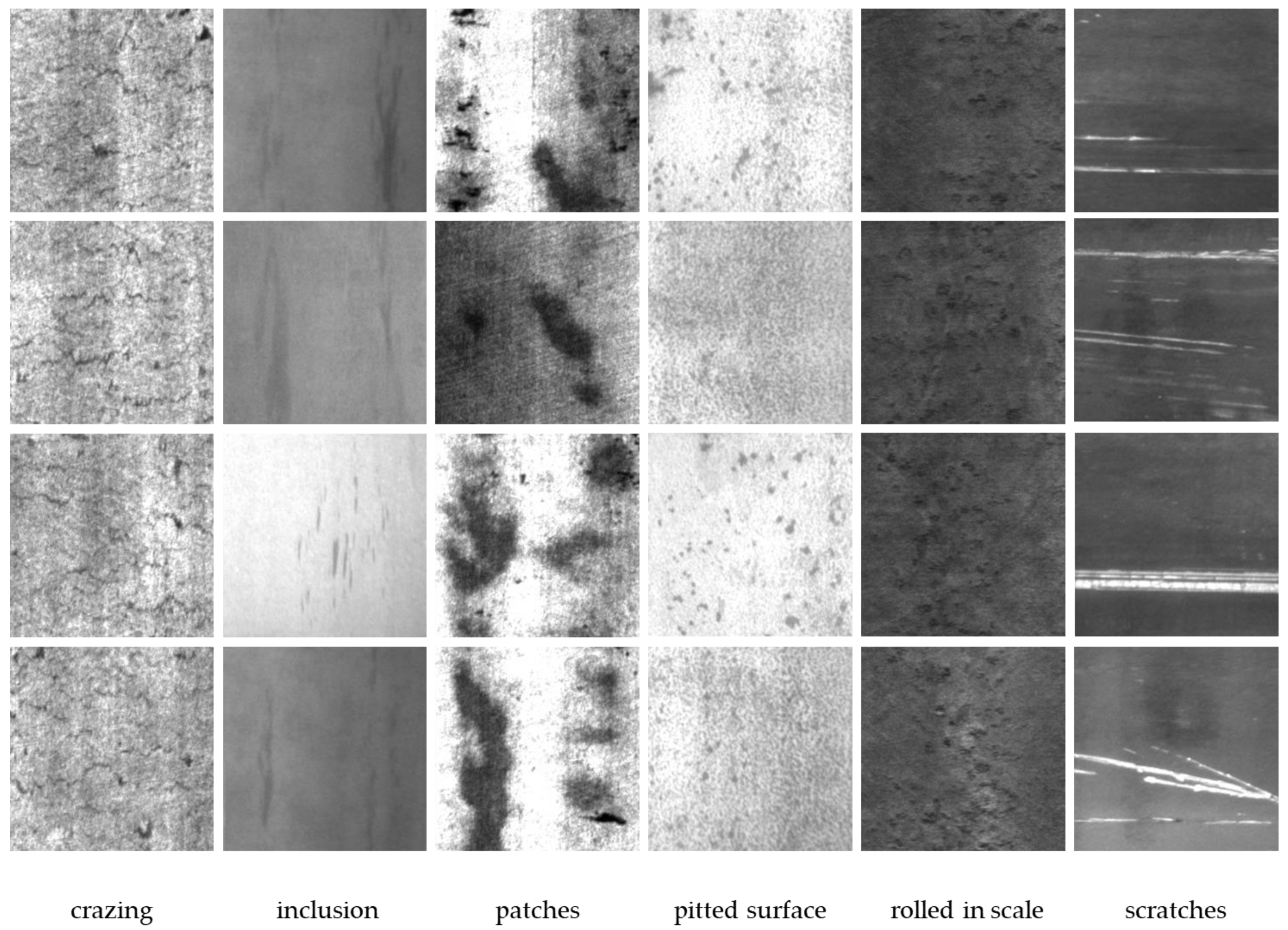
2.1.1. The NEU-DET Dataset
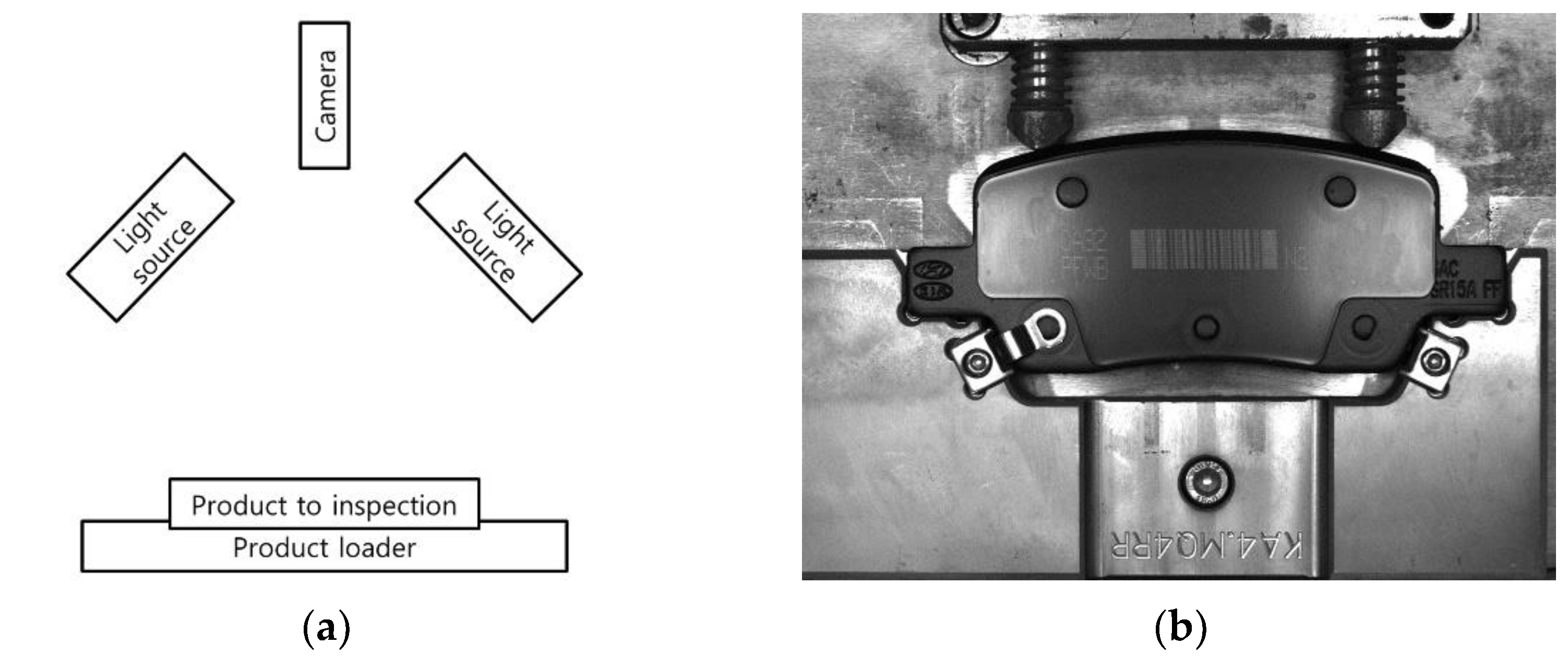
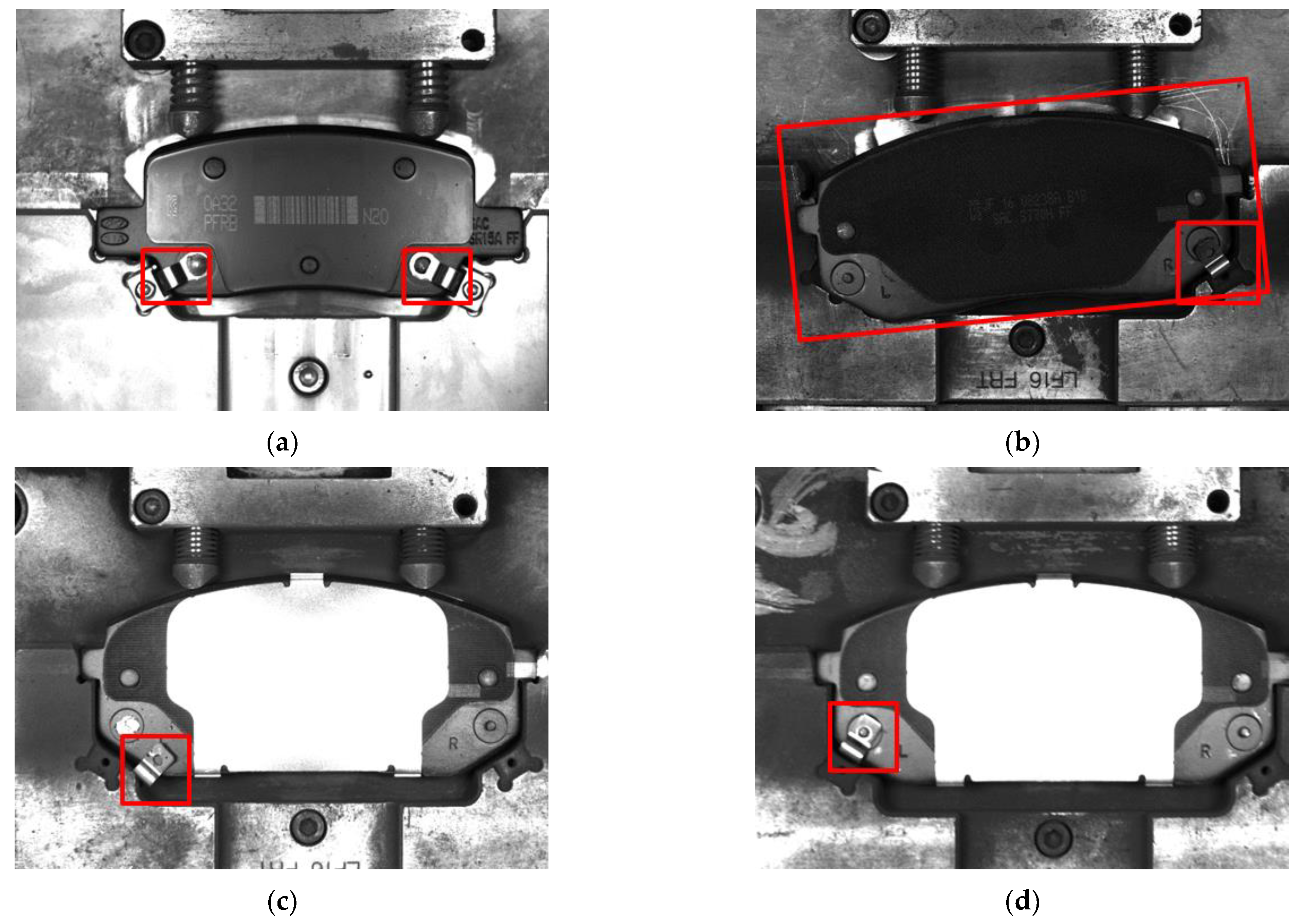
2.1.2. Brake Pad Dataset
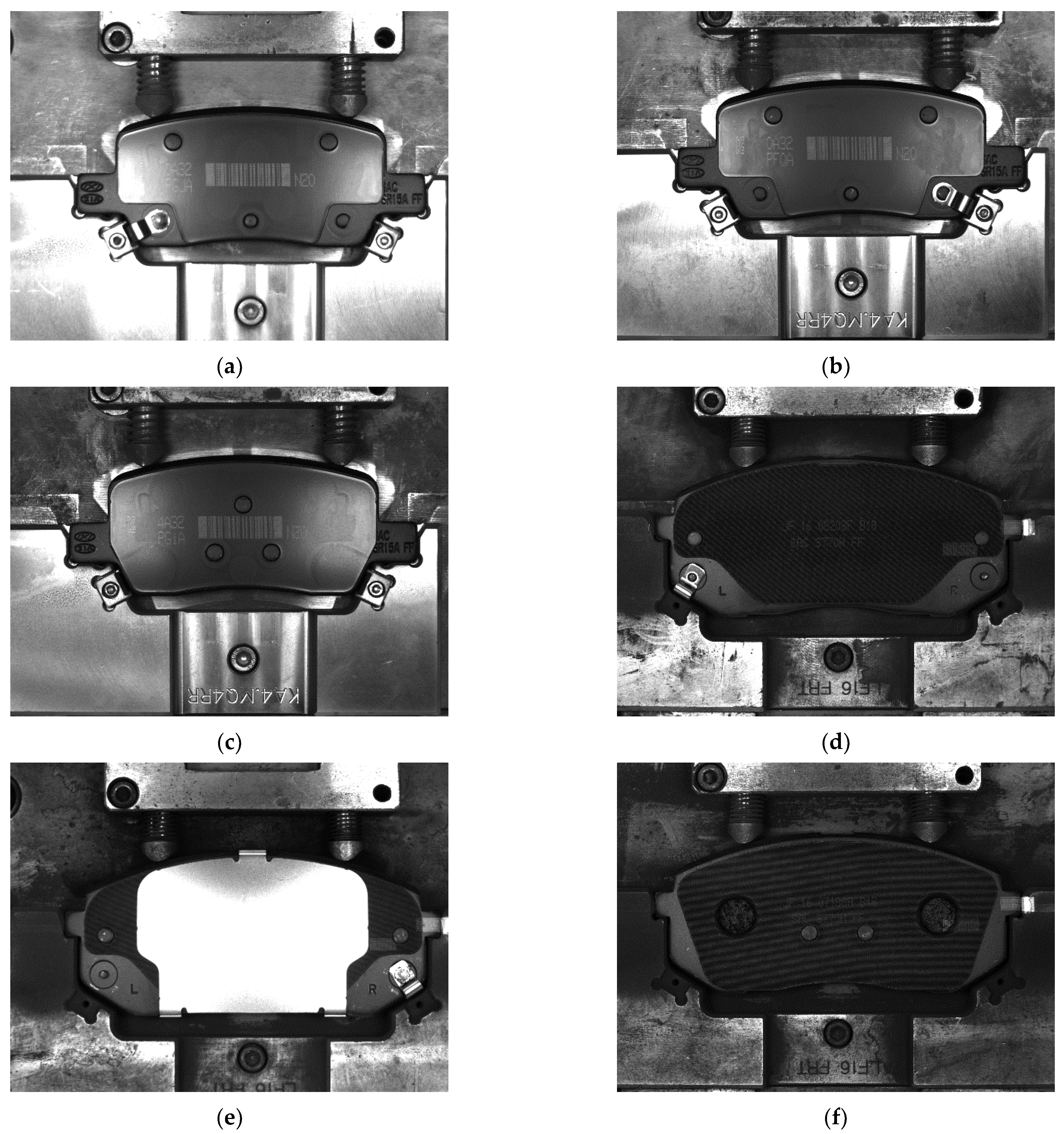
- Inspecting the location of the protruding part of the product to inspect whether the product is loaded in the wrong location, as shown in Figure 5b.
- Inspecting whether the metal sensor is located correctly in the specified location of the product, as shown in Figure 5a,c.
- Inspecting whether the riveting is performed correctly to secure the sensor. Figure 5d shows an incorrectly riveted product.
2.2. Proposed Data Augmentation Method
- Original images (original).
- Augmented one-channel grayscale images with original images (one-channel).
- Grayscale images were converted after augmentation, using the proposed method with original images (three-channel, gray).
- Color images augmented by using the proposed method with original images (three-channel, color).
2.2.1. One-Channel Augmentation
Pixel Noise
| Algorithm 1. Pseudo-code of applying pixel noise to the given image. |
| Input: Original grayscale image Output: Grayscale image with pixel noise. for x in range of 0 to width of image for y in range of 0 to height of image value = image[x, y] + random number in range of −10 to 10 if value > 255 value = 255 else if value < 0 value = 0 image[x, y] = value end for end for |
Contrast Limited Adaptive Histogram Equalization (CLAHE)
Gaussian Blur
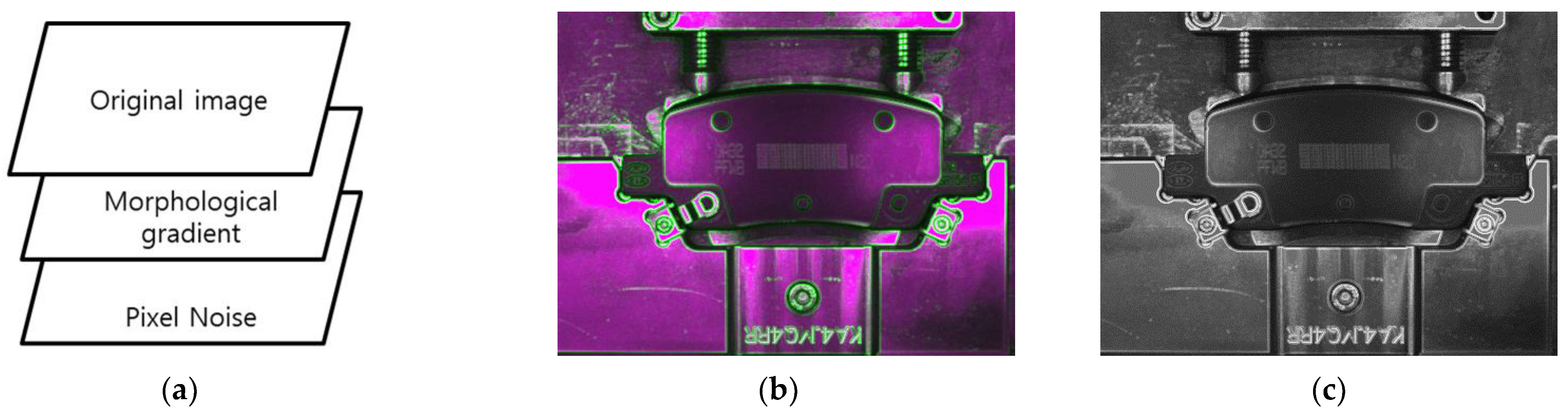
Morphological Gradient
2.2.2. Three-Channel Augmentation
2.3. Networks
2.3.1. Image Classification Networks
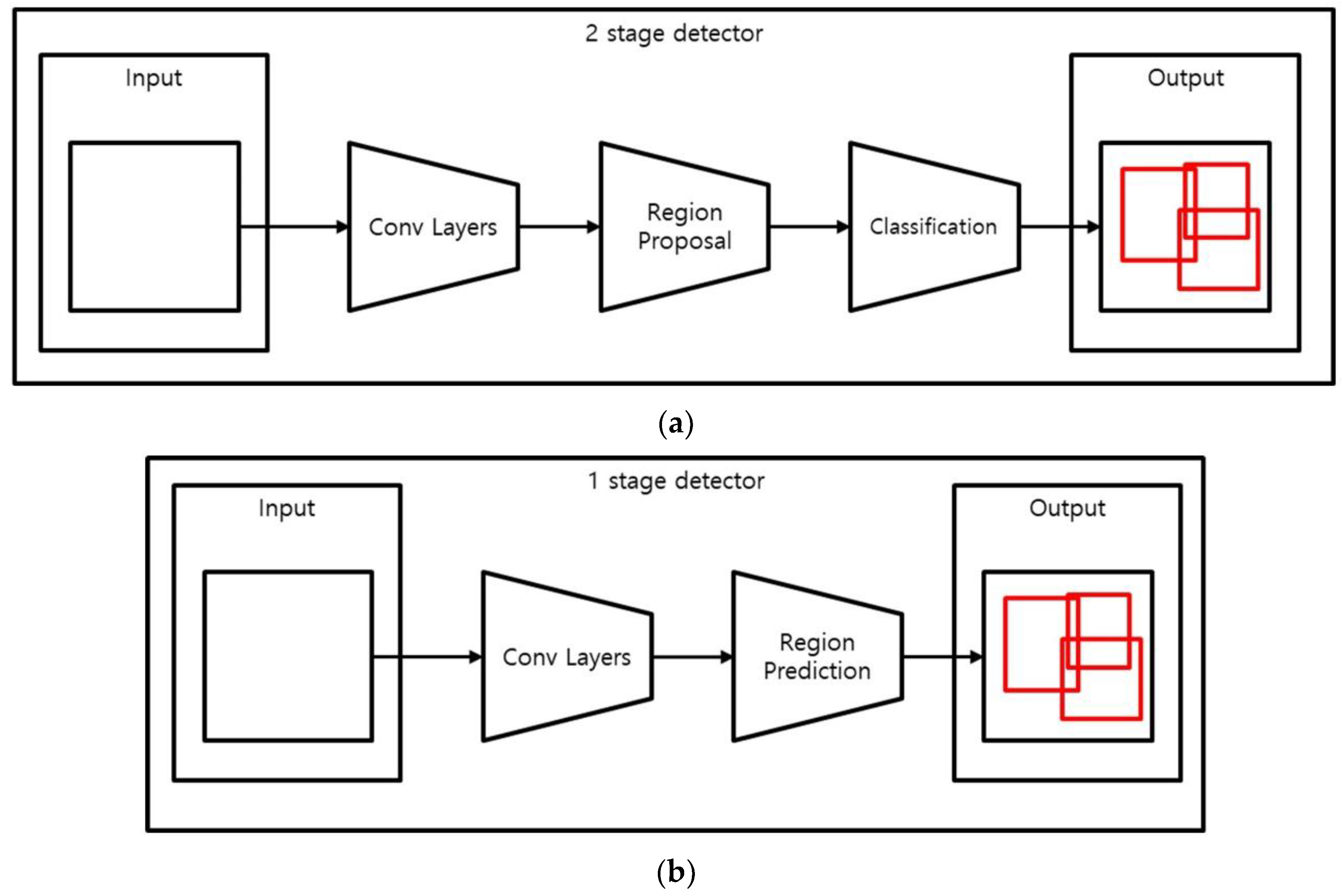
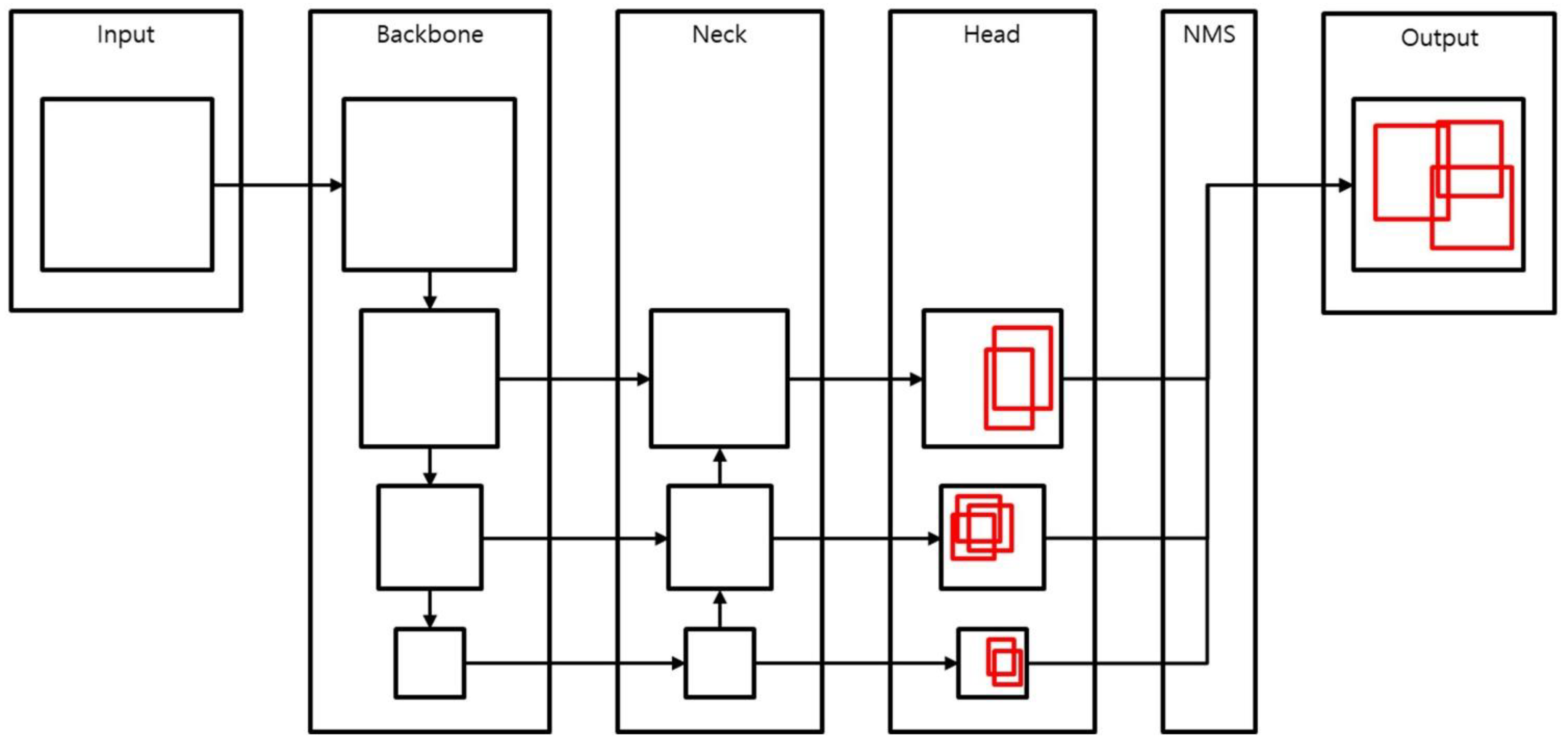
2.3.2. Object Detection Networks
3. Results
3.1. Evaluation Metrics
3.1.1. Image Classification Metrics
3.1.2. Object Detection Metrics
3.2. Quantitative Results
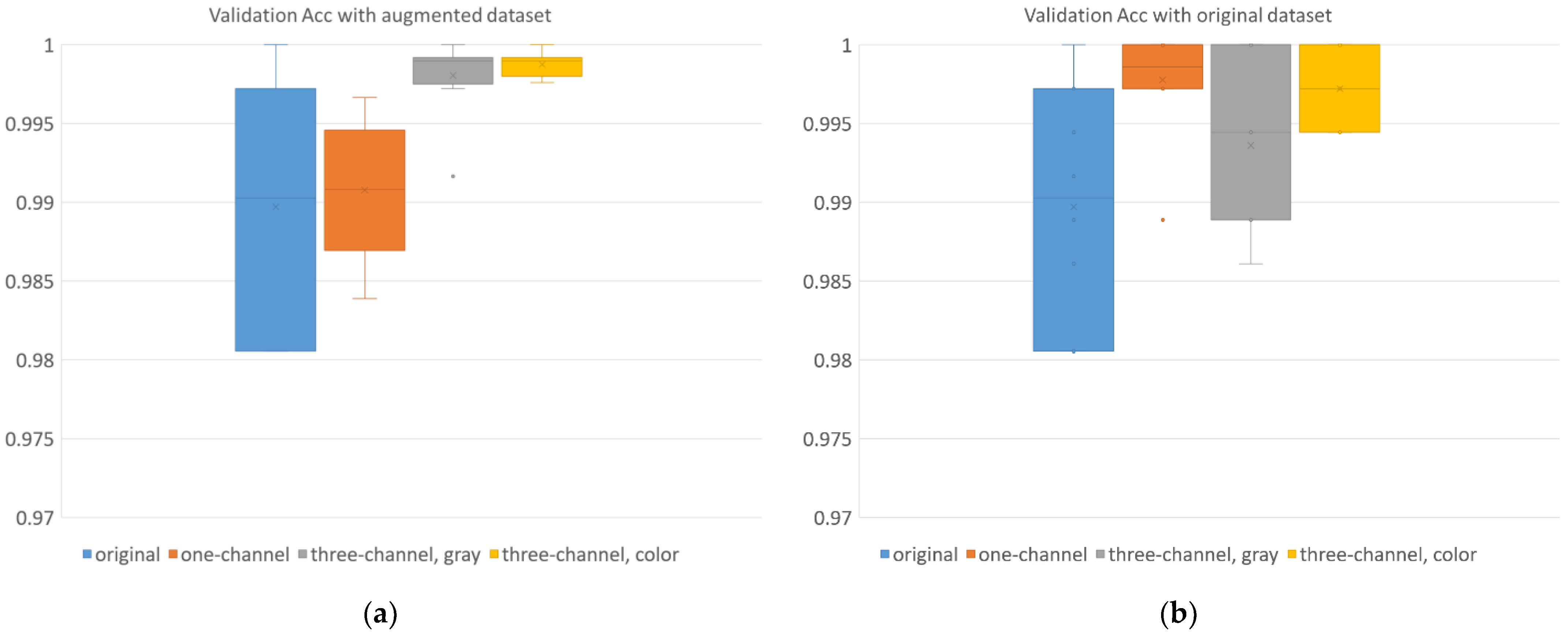
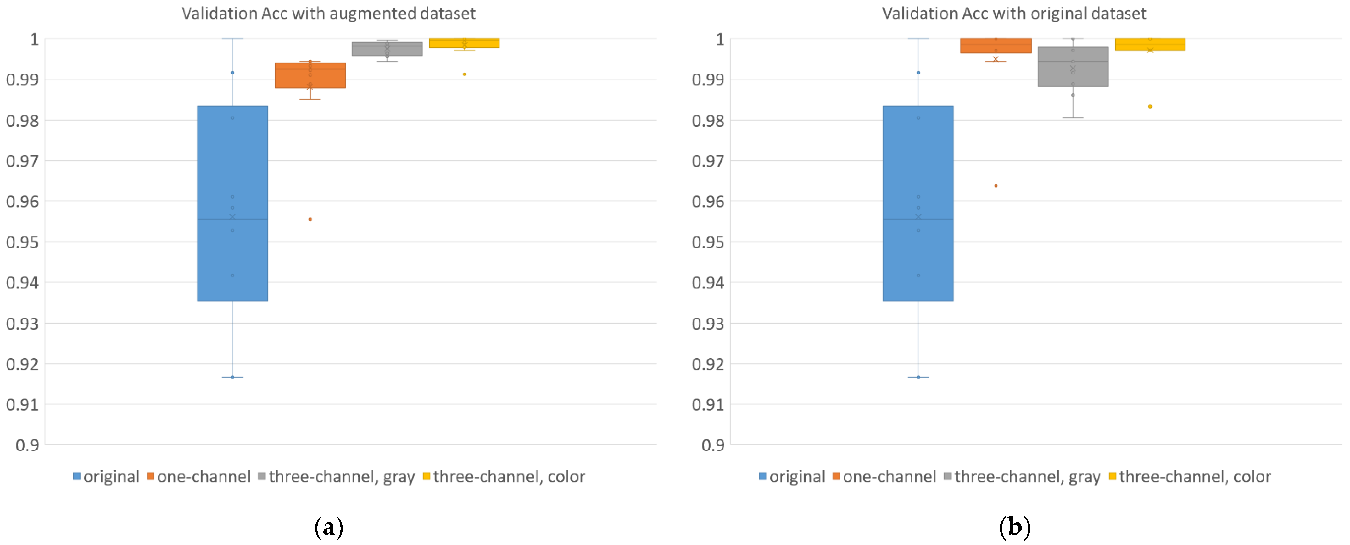
3.2.1. Image Classification
MobileNetV2 Results
Resnet18 Results
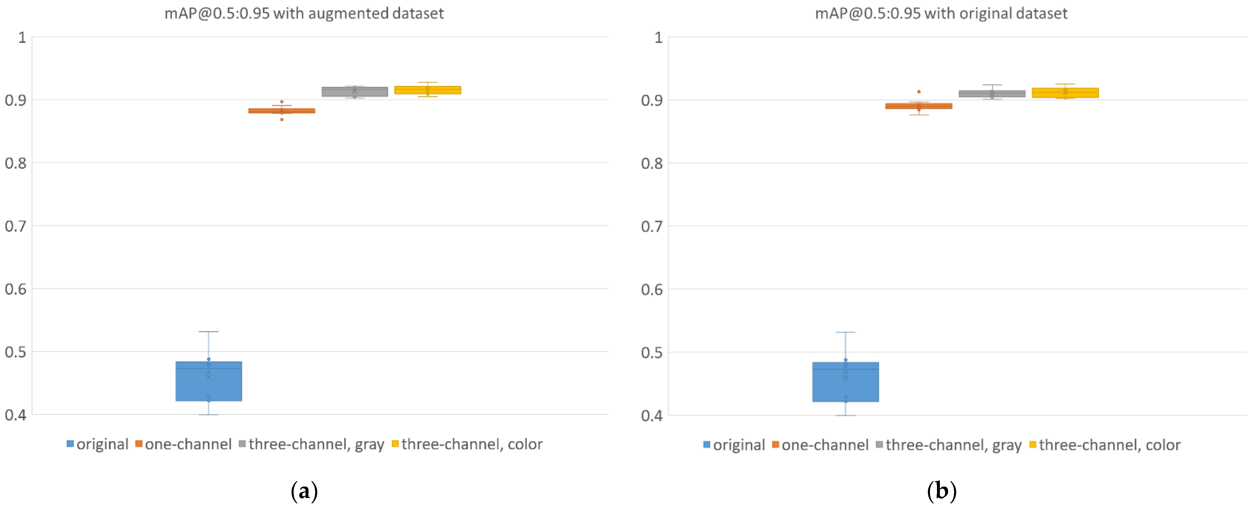
3.2.2. Object Detection
YOLOv4 Results
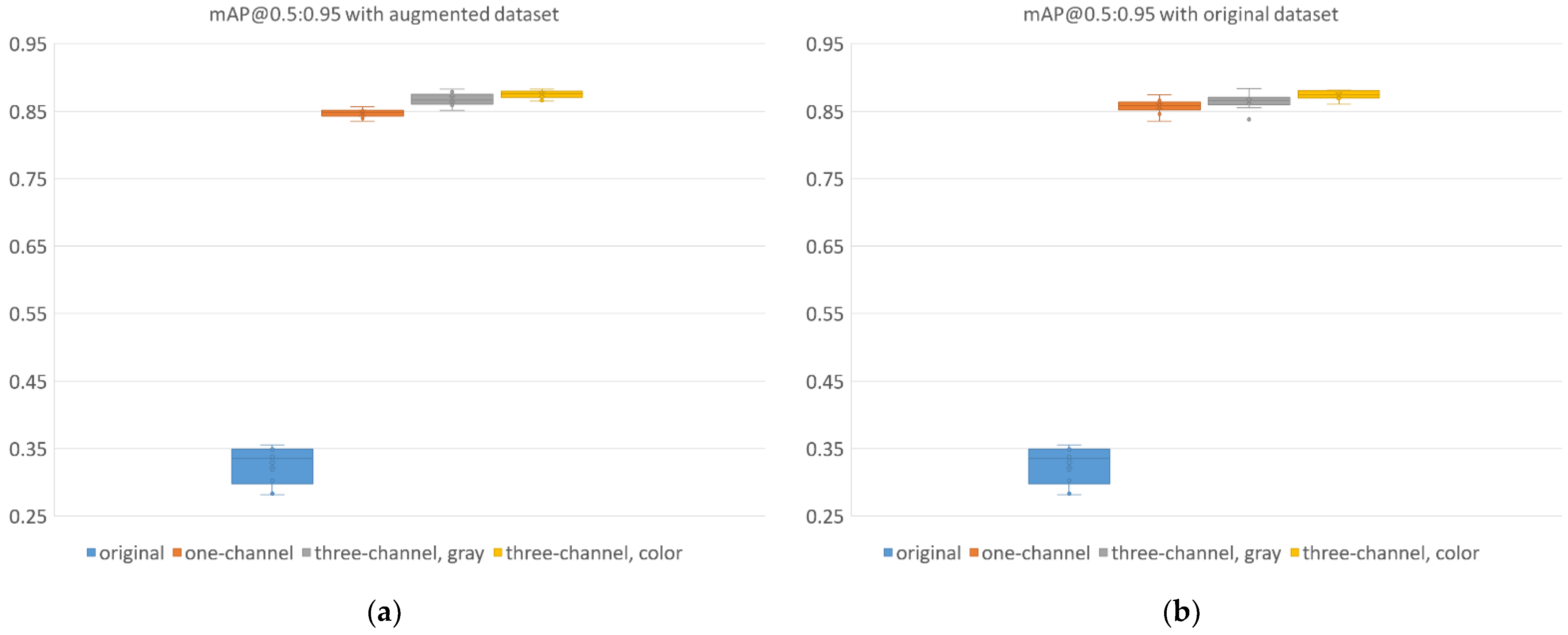
YOLOv4-Tiny Results
4. Discussion
5. Conclusions
Author Contributions
Funding
Institutional Review Board Statement
Informed Consent Statement
Data Availability Statement
Conflicts of Interest
References
- Jiang, B.; Wang, C.-C.; Tsai, D.-M.; Lu, C.-J. LCD surface defect inspection using machine vision. In Proceedings of the Fifth Asia Pacific Industrial Engineering and Management Systems Conference, Gold Coast, Australia, 12–15 December 2004; pp. 24.7.1–24.7.9. [Google Scholar]
- Böttger, T.; Ulrich, M. Real-time texture error detection on textured surfaces with compressed sensing. Pattern Recognit. Image Anal. 2016, 26, 88–94. [Google Scholar] [CrossRef]
- Song, K.; Yan, Y. A noise robust method based on completed local binary patterns for hot-rolled steel strip surface defects. Appl. Surf. Sci. 2013, 285, 858–864. [Google Scholar] [CrossRef]
- Krizhevsky, A.; Sutskever, I.; Hinton, G.E. ImageNet classification with deep convolutional neural networks. In Proceedings of the 25th International Conference on Neural Information Processing Systems-Volume 1, Lake Tahoe, NV, USA, 3–6 December 2012; pp. 1097–1105. [Google Scholar]
- Bergmann, P.; Fauser, M.; Sattlegger, D.; Steger, C. MVTec AD—A Comprehensive Real-World Dataset for Unsupervised Anomaly Detection. In Proceedings of the 2019 IEEE/CVF Conference on Computer Vision and Pattern Recognition (CVPR), Long Beach, CA, USA, 15–20 June 2019; pp. 9584–9592. [Google Scholar]
- Chang, F.; Liu, M.; Dong, M.; Duan, Y. A mobile vision inspection system for tiny defect detection on smooth car-body surfaces based on deep ensemble learning. Meas. Sci. Technol. 2019, 30. [Google Scholar] [CrossRef]
- Chien, J.-C.; Wu, M.-T.; Lee, J.-D. Inspection and Classification of Semiconductor Wafer Surface Defects Using CNN Deep Learning Networks. Appl. Sci. 2020, 10, 5340. [Google Scholar] [CrossRef]
- Ding, F.; Zhuang, Z.; Liu, Y.; Jiang, D.; Yan, X.; Wang, Z. Detecting Defects on Solid Wood Panels Based on an Improved SSD Algorithm. Sensors 2020, 20, 5315. [Google Scholar] [CrossRef]
- Lin, J.; Yao, Y.; Ma, L.; Wang, Y. Detection of a casting defect tracked by deep convolution neural network. Int. J. Adv. Manuf. Technol. 2018, 97, 573–581. [Google Scholar] [CrossRef]
- Lu, M.; Chen, C.-L. Detection and Classification of Bearing Surface Defects Based on Machine Vision. Appl. Sci. 2021, 11, 1825. [Google Scholar] [CrossRef]
- Ruiz, L.; Torres, M.; Gómez, A.; Díaz, S.; González, J.M.; Cavas, F. Detection and Classification of Aircraft Fixation Elements during Manufacturing Processes Using a Convolutional Neural Network. Appl. Sci. 2020, 10, 6856. [Google Scholar] [CrossRef]
- Sun, X.; Gu, J.; Huang, R.; Zou, R.; Giron Palomares, B. Surface Defects Recognition of Wheel Hub Based on Improved Faster R-CNN. Electronics 2019, 8, 481. [Google Scholar] [CrossRef] [Green Version]
- Urbonas, A.; Raudonis, V.; Maskeliūnas, R.; Damaševičius, R. Automated Identification of Wood Veneer Surface Defects Using Faster Region-Based Convolutional Neural Network with Data Augmentation and Transfer Learning. Appl. Sci. 2019, 9, 4898. [Google Scholar] [CrossRef] [Green Version]
- Wang, T.; Chen, Y.; Qiao, M.N.; Snoussi, H. A fast and robust convolutional neural network-based defect detection model in product quality control. Int. J. Adv. Manuf Tech. 2018, 94, 3465–3471. [Google Scholar] [CrossRef]
- Wen, S.; Chen, Z.; Li, C. Vision-Based Surface Inspection System for Bearing Rollers Using Convolutional Neural Networks. Appl. Sci. 2018, 8, 2565. [Google Scholar] [CrossRef] [Green Version]
- Yang, Y.; Pan, L.; Ma, J.; Yang, R.; Zhu, Y.; Yang, Y.; Zhang, L. A High-Performance Deep Learning Algorithm for the Automated Optical Inspection of Laser Welding. Appl. Sci. 2020, 10, 933. [Google Scholar] [CrossRef] [Green Version]
- Yun, J.P.; Shin, W.C.; Koo, G.; Kim, M.S.; Lee, C.; Lee, S.J. Automated defect inspection system for metal surfaces based on deep learning and data augmentation. J. Manuf. Syst. 2020, 55, 317–324. [Google Scholar] [CrossRef]
- Zhang, J.; Liu, H.; Cao, J.; Zhu, W.; Jin, B.; Li, W. A Deep Learning Based Dislocation Detection Method for Cylindrical Crystal Growth Process. Appl. Sci. 2020, 10, 7799. [Google Scholar] [CrossRef]
- He, Y.; Song, K.; Meng, Q.; Yan, Y. An End-to-End Steel Surface Defect Detection Approach via Fusing Multiple Hierarchical Features. IEEE Trans. Instrum. Meas. 2020, 69, 1493–1504. [Google Scholar] [CrossRef]
- Lv, X.; Duan, F.; Jiang, J.-J.; Fu, X.; Gan, L. Deep Active Learning for Surface Defect Detection. Sensors 2020, 20, 1650. [Google Scholar] [CrossRef] [Green Version]
- Yang, J.; Li, S.; Wang, Z.; Dong, H.; Wang, J.; Tang, S. Using Deep Learning to Detect Defects in Manufacturing: A Comprehensive Survey and Current Challenges. Materials 2020, 13, 5755. [Google Scholar] [CrossRef] [PubMed]
- Xie, Y.; Richmond, D. Pre-training on Grayscale ImageNet Improves Medical Image Classification. In Proceedings of the European Conference on Computer Vision (ECCV) Workshops, Munich, Germany, 8–14 September 2018; pp. 476–484. [Google Scholar]
- Burduja, M.; Ionescu, R.T.; Verga, N. Accurate and Efficient Intracranial Hemorrhage Detection and Subtype Classification in 3D CT Scans with Convolutional and Long Short-Term Memory Neural Networks. Sensors 2020, 20, 5611. [Google Scholar] [CrossRef]
- Lin, T.-Y.; Maire, M.; Belongie, S.; Hays, J.; Perona, P.; Ramanan, D.; Dollár, P.; Zitnick, C.L. Microsoft COCO: Common Objects in Context. In Lecture Notes in Computer Science, Proceedings of the European Conference on Computer Vision, Zurich, Switzerland, 6–12 September 2014; Springer: Cham, Switzerland, 2014; pp. 740–755. [Google Scholar]
- Pizer, S.M.; Johnston, R.E.; Ericksen, J.P.; Yankaskas, B.C.; Muller, K.E. Contrast-limited adaptive histogram equalization: Speed and effectiveness. In Proceedings of the First Conference on Visualization in Biomedical Computing, Atlanta, GA, USA, 22–25 May 1990; pp. 337–345. [Google Scholar]
- Canny, J. A Computational Approach to Edge Detection. IEEE Trans. Pattern Anal. Mach. Intell. 1986, PAMI-8, 679–698. [Google Scholar] [CrossRef]
- Sandler, M.; Howard, A.; Zhu, M.; Zhmoginov, A.; Chen, L.-C. MobileNetV2: Inverted Residuals and Linear Bottlenecks. arXiv 2018, arXiv:1801.04381. [Google Scholar]
- He, K.; Zhang, X.; Ren, S.; Sun, J. Deep Residual Learning for Image Recognition. arXiv 2015, arXiv:1512.03385. [Google Scholar]
- Bochkovskiy, A.; Wang, C.-Y.; Liao, H.-Y.M. YOLOv4: Optimal Speed and Accuracy of Object Detection. arXiv 2020, arXiv:2004.10934. [Google Scholar]
- Everingham, M.; Van Gool, L.; Williams, C.K.I.; Winn, J.; Zisserman, A. The Pascal Visual Object Classes (VOC) Challenge. Int. J. Comput. Vis. 2010, 88, 303–338. [Google Scholar] [CrossRef] [Green Version]


| Protruding Part | Unriveted Sensor | Riveted Sensor | |
|---|---|---|---|
| Training dataset | 1236 | 320 | 112 |
| Validation dataset | 138 | 37 | 12 |
| Augmentation Methods | Data Augmentation Methods of Each Image |
|---|---|
| One-channel Augmentation | Pixel Noise |
| CLAHE | |
| Gaussian Blur | |
| Morphological gradient | |
| Three-channel Augmentation | Original + Morphological gradient + Pixel noise |
| Original + Morphological gradient + Gaussian blur | |
| Original + Morphological gradient + CLAHE | |
| Pixel noise + Morphological gradient + Gaussian blur | |
| Pixel noise + Morphological gradient + CLAHE | |
| Gaussian blur + Morphological gradient + CLAHE |
| Dataset Configuration | # of Training Datasets | # of Validation Datasets |
|---|---|---|
| Original dataset | 240 | 60 |
| Original dataset + one-channel mixed dataset | 1200 | 300 |
| Original dataset + three-channel mixed dataset | 1680 | 420 |
| Dataset Configuration | # of Training Datasets | # of Validation Datasets |
|---|---|---|
| Original dataset | 490 | 55 |
| Original dataset + one-channel mixed dataset | 2450 | 275 |
| Original dataset + three-channel mixed dataset | 3430 | 385 |
| Learning Rate | Batch Size | Optimizer | Epochs |
|---|---|---|---|
| 0.001 | 16 | SGD | 2 |
| Networks | Learning Rate | Batch Size | Subdivisions | Epochs |
|---|---|---|---|---|
| YOLOv4 | 0.0013 | 64 | 32 | 10 |
| YOLOv4-tiny | 0.00261 | 64 | 16 | 10 |
| Prediction | |||
|---|---|---|---|
| Positive | Negative | ||
| Ground truth | Positive | TP (true positive) | FN (false negative) |
| Negative | FP (false positive) | TN (true negative) | |
| Original | One-Channel | Three-Channel Grayscale | Three-Channel Color | ||||||
|---|---|---|---|---|---|---|---|---|---|
| Mean | SD | Mean | SD | Mean | SD | Mean | SD | ||
| Augmented dataset | accuracy | 0.990 | 0.008 | 0.991 | 0.004 | 0.998 | 0.002 | 0.999 | 0.001 |
| F1 score | 0.990 | 0.007 | 0.991 | 0.004 | 0.998 | 0.002 | 0.999 | 0.001 | |
| Original dataset | accuracy | 0.990 | 0.008 | 0.998 | 0.003 | 0.994 | 0.002 | 0.997 | 0.002 |
| F1 score | 0.990 | 0.007 | 0.998 | 0.003 | 0.994 | 0.005 | 0.997 | 0.002 | |
| Original | One-Channel | Three-Channel Grayscale | Three-Channel Color | ||||||
|---|---|---|---|---|---|---|---|---|---|
| Mean | SD | Mean | SD | Mean | SD | Mean | SD | ||
| Augmented dataset | accuracy | 0.956 | 0.029 | 0.988 | 0.012 | 0.998 | 0.002 | 0.998 | 0.003 |
| F1 score | 0.960 | 0.025 | 0.988 | 0.011 | 0.998 | 0.002 | 0.998 | 0.003 | |
| Original dataset | accuracy | 0.956 | 0.029 | 0.995 | 0.011 | 0.993 | 0.002 | 0.997 | 0.005 |
| F1 score | 0.960 | 0.025 | 0.995 | 0.010 | 0.993 | 0.006 | 0.997 | 0.005 | |
| Original | One-Channel | Three-Channel Grayscale | Three-Channel Color | |||||
|---|---|---|---|---|---|---|---|---|
| Mean | SD | Mean | SD | Mean | SD | Mean | SD | |
| mAP@0.5 | 0.894 | 0.044 | 1.000 | 0.000 | 1.000 | 0.000 | 1.000 | 0.000 |
| mAP@0.55 | 0.857 | 0.072 | 1.000 | 0.000 | 1.000 | 0.000 | 1.000 | 0.000 |
| mAP@0.6 | 0.817 | 0.079 | 1.000 | 0.000 | 1.000 | 0.000 | 1.000 | 0.000 |
| mAP@0.65 | 0.727 | 0.092 | 1.000 | 0.000 | 1.000 | 0.000 | 1.000 | 0.000 |
| mAP@0.7 | 0.588 | 0.101 | 1.000 | 0.000 | 1.000 | 0.000 | 1.000 | 0.000 |
| mAP@0.75 | 0.397 | 0.049 | 0.998 | 0.001 | 1.000 | 0.001 | 1.000 | 0.000 |
| mAP@0.8 | 0.224 | 0.061 | 0.986 | 0.010 | 0.996 | 0.001 | 0.997 | 0.001 |
| mAP@0.85 | 0.077 | 0.033 | 0.963 | 0.016 | 0.989 | 0.001 | 0.988 | 0.001 |
| mAP@0.9 | 0.016 | 0.015 | 0.726 | 0.030 | 0.884 | 0.026 | 0.884 | 0.018 |
| mAP@0.95 | 0.001 | 0.001 | 0.150 | 0.062 | 0.272 | 0.069 | 0.293 | 0.063 |
| mAP@0.5:0.95 | 0.460 | 0.040 | 0.882 | 0.008 | 0.914 | 0.007 | 0.916 | 0.007 |
| Original | One-Channel | Three-Channel Grayscale | Three-Channel Color | |||||
|---|---|---|---|---|---|---|---|---|
| Mean | SD | Mean | SD | Mean | SD | Mean | SD | |
| mAP@0.5 | 0.894 | 0.044 | 1.000 | 0.000 | 1.000 | 0.000 | 1.000 | 0.000 |
| mAP@0.55 | 0.857 | 0.072 | 1.000 | 0.000 | 1.000 | 0.000 | 1.000 | 0.000 |
| mAP@0.6 | 0.817 | 0.079 | 1.000 | 0.000 | 1.000 | 0.000 | 1.000 | 0.000 |
| mAP@0.65 | 0.727 | 0.092 | 1.000 | 0.000 | 1.000 | 0.000 | 1.000 | 0.000 |
| mAP@0.7 | 0.588 | 0.101 | 1.000 | 0.000 | 1.000 | 0.000 | 1.000 | 0.000 |
| mAP@0.75 | 0.397 | 0.049 | 0.999 | 0.002 | 0.999 | 0.001 | 1.000 | 0.000 |
| mAP@0.8 | 0.224 | 0.061 | 0.986 | 0.016 | 0.996 | 0.001 | 0.997 | 0.000 |
| mAP@0.85 | 0.077 | 0.033 | 0.972 | 0.017 | 0.989 | 0.001 | 0.988 | 0.002 |
| mAP@0.9 | 0.016 | 0.015 | 0.767 | 0.022 | 0.885 | 0.034 | 0.860 | 0.045 |
| mAP@0.95 | 0.001 | 0.001 | 0.192 | 0.086 | 0.234 | 0.052 | 0.275 | 0.064 |
| mAP@0.5:0.95 | 0.460 | 0.040 | 0.892 | 0.009 | 0.910 | 0.007 | 0.912 | 0.008 |
| Original | One-Channel | Three-Channel Grayscale | Three-Channel Color | |||||
|---|---|---|---|---|---|---|---|---|
| Mean | SD | Mean | SD | Mean | SD | Mean | SD | |
| mAP@0.5 | 0.857 | 0.044 | 1.000 | 0.000 | 1.000 | 0.000 | 1.000 | 0.000 |
| mAP@0.55 | 0.761 | 0.067 | 1.000 | 0.000 | 1.000 | 0.000 | 1.000 | 0.000 |
| mAP@0.6 | 0.620 | 0.080 | 1.000 | 0.000 | 1.000 | 0.000 | 1.000 | 0.000 |
| mAP@0.65 | 0.464 | 0.075 | 1.000 | 0.000 | 1.000 | 0.000 | 1.000 | 0.000 |
| mAP@0.7 | 0.306 | 0.061 | 1.000 | 0.000 | 1.000 | 0.000 | 1.000 | 0.000 |
| mAP@0.75 | 0.160 | 0.045 | 0.997 | 0.002 | 0.997 | 0.003 | 0.999 | 0.001 |
| mAP@0.8 | 0.070 | 0.019 | 0.979 | 0.005 | 0.988 | 0.004 | 0.985 | 0.004 |
| mAP@0.85 | 0.013 | 0.009 | 0.897 | 0.019 | 0.954 | 0.005 | 0.958 | 0.009 |
| mAP@0.9 | 0.001 | 0.001 | 0.548 | 0.039 | 0.657 | 0.054 | 0.717 | 0.043 |
| mAP@0.95 | 0.000 | 0.000 | 0.050 | 0.027 | 0.081 | 0.040 | 0.092 | 0.031 |
| mAP@0.5:0.95 | 0.325 | 0.028 | 0.847 | 0.006 | 0.868 | 0.009 | 0.875 | 0.006 |
| Original | One-Channel | Three-Channel Grayscale | Three-Channel Color | |||||
|---|---|---|---|---|---|---|---|---|
| Mean | SD | Mean | SD | Mean | SD | Mean | SD | |
| mAP@0.5 | 0.857 | 0.044 | 1.000 | 0.000 | 1.000 | 0.000 | 1.000 | 0.000 |
| mAP@0.55 | 0.761 | 0.067 | 1.000 | 0.000 | 1.000 | 0.000 | 1.000 | 0.000 |
| mAP@0.6 | 0.620 | 0.080 | 1.000 | 0.000 | 1.000 | 0.000 | 1.000 | 0.000 |
| mAP@0.65 | 0.464 | 0.075 | 1.000 | 0.000 | 1.000 | 0.000 | 1.000 | 0.000 |
| mAP@0.7 | 0.306 | 0.061 | 1.000 | 0.000 | 1.000 | 0.001 | 1.000 | 0.000 |
| mAP@0.75 | 0.160 | 0.045 | 0.996 | 0.003 | 0.999 | 0.003 | 0.998 | 0.002 |
| mAP@0.8 | 0.070 | 0.019 | 0.983 | 0.005 | 0.989 | 0.006 | 0.986 | 0.005 |
| mAP@0.85 | 0.013 | 0.009 | 0.923 | 0.029 | 0.939 | 0.017 | 0.951 | 0.015 |
| mAP@0.9 | 0.001 | 0.001 | 0.593 | 0.049 | 0.645 | 0.079 | 0.704 | 0.050 |
| mAP@0.95 | 0.000 | 0.000 | 0.077 | 0.052 | 0.068 | 0.049 | 0.097 | 0.036 |
| mAP@0.5:0.95 | 0.325 | 0.028 | 0.857 | 0.011 | 0.864 | 0.012 | 0.874 | 0.007 |
Publisher’s Note: MDPI stays neutral with regard to jurisdictional claims in published maps and institutional affiliations. |
© 2021 by the authors. Licensee MDPI, Basel, Switzerland. This article is an open access article distributed under the terms and conditions of the Creative Commons Attribution (CC BY) license (https://creativecommons.org/licenses/by/4.0/).
Share and Cite
Wang, J.; Lee, S. Data Augmentation Methods Applying Grayscale Images for Convolutional Neural Networks in Machine Vision. Appl. Sci. 2021, 11, 6721. https://doi.org/10.3390/app11156721
Wang J, Lee S. Data Augmentation Methods Applying Grayscale Images for Convolutional Neural Networks in Machine Vision. Applied Sciences. 2021; 11(15):6721. https://doi.org/10.3390/app11156721
Chicago/Turabian StyleWang, Jinyeong, and Sanghwan Lee. 2021. "Data Augmentation Methods Applying Grayscale Images for Convolutional Neural Networks in Machine Vision" Applied Sciences 11, no. 15: 6721. https://doi.org/10.3390/app11156721