LAMDA Controller Applied to the Trajectory Tracking of an Aerial Manipulator

Abstract

In this work, a novel LAMDA (Learning Algorithm for Multivariable Data Analysis) control strategy for trajectory tracking for an aerial manipulator is presented. Four control strategies are developed: Kinematic, Inverse Dynamics, Sliding Mode (SMC), and LAMDA. These are compared with each other in order to verify their performance to fulfill the control objective. Experimental tests were also carried out to validate the developed controllers. In addition, a study of stability has been also performed for all the controllers. The results obtained by the LAMDA controller demonstrated the good performance of the controller in the aerial manipulator robot. To the best of our knowledge, this is the first time a LAMDA controller has been applied to an aerial robotic manipulator.

1. Introduction

At present, the characteristics of the aerial manipulator have been used in multiple applications, because the mobility of the hexacopter and the maneuverability of the robotic arm make it very useful [1,2,3]. The first works are oriented to the development of applications considering only the kinematics of the aerial manipulator, i.e., coriolis forces, mass inertia, etc., are not considered. In this context, several research studies on aerial manipulators have been presented, for example, an algorithm for the control of a contact inspection for an unmanned aerial vehicle (UAV) manipulator [4], or a trajectory-tracking control algorithm for the parallel aerial manipulator based on the Stewart platform [5]. Guayasamín et al. [6] designed a trajectory tracking control based on the Lyapunov and Sliding Mode Control (SMC) theory applied to a Kinematic model. In the same line, predictive control for trajectory tracking has been included for a two-armed aerial manipulator [7]. In the work of Yarai et al. [8], the dynamics of the robotic arm is taken as an external perturbation and a decoupling controller is proposed to guarantee that the dynamics produced by the robotic arm to the quadrotor (and vice versa) are not part of the quadrotor dynamics. Wang et al. [9] designed a Sliding Mode controller to track the trajectory of the spatial manipulator, and a linear quadratic regulator (LQR) controller of the subsystem was designed to suppress the vibration of the flexible components. A null-space-based controller has been defined for a group of aerial manipulators [10].

The previous studies only contemplate the kinematics of the aerial manipulator. However, in real applications, it is necessary to consider the mass, inertia, friction forces, perturbations, etc. These characteristics require other types of controllers to compensate the dynamics of the system. Thus, several works have been developed to solve this problem, like the work of Gkountas and Tzes [11] who presented the modeling and control of unmanned aerial manipulators (UAM) in a leader–follower configuration that performed a cooperative manipulation task taking into account the dynamics of the system. In the study of Morton et al. [12] the dynamics were compensated with an inverse dynamics controller for trajectory tracking.

Different control algorithms have been developed to improve the performance of aerial manipulators robots. For example, a controller based on neural networks was implemented for trajectory tracking with the dynamic model [13]. In the same context, a controller based on null space to coordinate a group of robots was presented in [14]. An adaptive position control was implemented by Liu and Huang [15] aimed at compensating for certain perturbations in the modeling of the aerial manipulator, whereas a feedback control strategy was presented by Naldi et al. [16] allowing both the position and orientation of the end-effector to follow a desired trajectory considering the manipulator dynamics. The abovementioned research considers the control of an aerial manipulator from the point of view of its dynamics. In order to carry this out, the search for new controllers that can include the dynamics of aerial manipulators robots, meet the control objectives, and improve the performance of the task is vital for researchers.

Artificial intelligence (AI) approaches help to improve the behavior of the controllers. Among others, the fuzzy logic allows obtaining good results when the plant model is inaccurate or is not known in detail, which usually arises in the field of robotics. One of these methods is LAMDA (Learning Algorithm for Multivariable Data Analysis), which has been designed originally for classification and clustering tasks [17,18,19,20]. For example, a LAMDA fuzzy classification technique has been implemented to interpret the behavior of a drinking water treatment plant [21]. Recently, the use of the LAMDA features (in the detection of functional states of systems) has been proposed to make it work as a controller. For example, a class-based LAMDA controller was proposed and validated in the regulation of humidity and temperature of a complex Heating, Ventilation, and Air-Conditioning (HVAC) system in [22], obtaining excellent performance when considering that the mathematical model of the plant was variable or inexact. In [23], an adaptive LAMDA has been proposed and formalized for the control and modeling of systems, modifying the LAMDA structure with the addition of layers operating similar to neural networks, but with the advantage of having a fixed number of layers whose calibration is not trivial. This controller has proven to be adequate where the system dynamics are uncertain and complex. Finally, previous work [24] focuses on the formalization of a LAMDA algorithm for control based on the fundamentals of the Lyapunov theory and the Sliding-Mode Control (SMC), to guarantee stability and robustness of the overall system. The method is called LAMDA-SMC (LSMC) and takes advantage of LAMDA features to design a chattering-free controller. LSMC has been tested in the field of control of chemical processes, demonstrating that it is stable in the control of systems with model uncertainties and under disturbances. The results obtained by this LAMDA controller have been good in non-robotic aerial applications.

• The originality of this article lies in the validation of the robust LAMDA controller in aerial robotic systems whose dynamics are partially known or inaccurate. The main features of the proposed method are the following:
• The controller is based on concepts derived from LAMDA theory: Classes or functional states have a number of fixed layers (intrinsic feature). Therefore, the design is more straightforward than methods where the number of internal layers must be calibrated.
• The proposed controller uses the class criteria, which allows a quick convergence on the desired output without requiring a learning method that increases computational time.
• The design of a controller where the continuous and discontinuous control actions of SMC schemes are computed using the LAMDA method.
• A comparative analysis between the LAMDA method that does not use the aerial manipulator robot model is carried out with other well-known controller, which depend on model. Thus, obtaining a good performance of the controller without considering of the dynamics system.

Based on the abovementioned features, the contribution of this article is the design of an intelligent controller based on the LAMDA fuzzy algorithm for the trajectory tracking of an aerial manipulator robot and validating the approach in this field of study. Four control algorithms will be designed: (i) Kinematic, (ii) Inverse Dynamics, (iii) SMC Sliding Mode, and (iv) LAMDA. Finally, experimental tests will be carried out for the four controllers on a real aerial manipulator robot with three degrees of freedom for trajectory-tracking purposes.

The paper is organized as follows: Section 2 presents the kinematic and dynamic robot model, whereas Section 3 describes the design of the four controllers as well as their stability. Experimental tests and analysis of the results are given in Section 4. Finally, discussion and main conclusions are presented in Section 5.

2. Aerial Manipulator Robot Model

The aerial manipulator robot consists of a robotic arm on a hexacopter. These robots can perform the most common missions of robotic systems that require both navigation and manipulation capabilities. In the current work, an aerial manipulator robot consisting of a hexacopter and a robotic arm is considered.

2.1. Kinematic Model

The aerial manipulator robot consists of a robotic arm located on hexacopter, as shown in Figure 1. In the configuration of the aerial manipulator robot the position and orientation of all its points with respect to an inertial reference system $ℛ\left(\mathcal{X},\mathcal{Y},\mathcal{Z}\right)$ is known. The configuration of the aerial manipulator robot is defined by a vector q(t) of n independent coordinates, which are called the generalized coordinates of the aerial manipulator robot, defined as $q\left(t\right)=\left[q_a q_Q\right]$ where $q_a$ are the velocities of hexacopter, and $q_Q$ are velocities of the robotic arm. The configuration of $q\left(t\right)$ is an element of the configuration space of the aerial manipulator robot represented by $\mathcal{N}$. The position of the aerial manipulator robot end-effector $\xi \left(t\right)=\left[{\xi }_1 {\xi }_2\dots {\xi }_m\right]$ is defined by an m-dimensional vector representing the orientation and position of the robot’s point of interest with respect to $\{ℛ\}$. The position of the end-effector with respect to $\{ℛ\}$ defines the operating space of the aerial manipulator robot, denoted by $ℳ$.

The direct kinematics of the aerial manipulator robot defines the position and orientation of the end-effector ξ(t) as a function of the configuration of the robotic arm and the hexacopter (or its operational coordinates as functions of the generalized coordinates of the robotic arm and the operational coordinates of the hexacopter).

$$f: {\mathcal{N}}_{a}x{\mathcal{N}}_{\mathcal{Q}}\to ℳ$$

(1)

$$\left(q_a\left(t\right), q_Q\left(t\right)\right)\to \xi \left(t\right)=f\left(q_a, q_Q\right)$$

(2)

The kinematic model of the aerial manipulator robot sets the derivative of the end-effector position as a function of the derivative of the configuration of the robotic arm and the hexacopter (or their operational velocities as functions of their generalized velocities).

$$\dot{\xi }\left(t\right)=\frac{\partial \left(q_a, q_Q\right)}{\partial q}\mu \left(t\right)$$

(3)

where $\dot{\xi }\left(t\right)$ = [${\dot{\xi }}_1 {\dot{\xi }}_2\dots {\dot{\xi }}_m]\in R^m$ represents the velocity vector of the end-effector with respect to the inertial reference system $\{ℛ\}$. Let $\mu \left(t\right)=\left[\dot{q_a} \dot{u}\right]$ be the maneuverability vector of the aerial manipulator robot. Considering $J\left(q\right)=\frac{\partial f}{\partial q}{\rm T}\left(q\right)$ in the previous equation, one has:

$$\dot{\xi }\left(t\right)=J\left(q\right)\mu \left(t\right)$$

(4)

where the Jacobian matrix $J\left(q_q, q_Q\right)$ defines the linear mapping between the aerial manipulator robot maneuverability vector $\mu \left(t\right)$ and the end-effector velocity vector $\dot{\xi }\left(t\right)$. ${\rm T}\left(q\right)$ is the transformation matrix relating the velocities of $\dot{q}\left(t\right)$ and the velocities of the aerial manipulator robot $\mu \left(t\right)$, in such a way that: $\dot{q}\left(t\right)={\rm T}\left(q\right)\mu \left(t\right)$.

It is essential to emphasize that the dimension of the operational space m is smaller than the aerial manipulator robot degree of freedom n ($m<n$. ), so the aerial manipulator robot is called a redundant system.

2.2. Dynamic Model

The dynamics of a system, as reviewed in the literature, is an important contribution in the implementation of control algorithms. Therefore, in this section, we present the dynamics of the aerial manipulator robot, by applying the Euler–Lagrange analysis, where

L = E_c − E_p

(5)

where $L$ is the Lagrangean, $E_c$ is the kinetic energy, and $E_p$ is the potential energy, and where $E_c$ y $E_p$ are functions of the masses of the links of robotic arm, mass of the hexacopter, lengths and dimensions, angular positions, and velocities of the aerial manipulator robot. It is known that the Lagrange equation is given by:

$$f=\frac{d}{dt}\left(\frac{dL}{d\dot{q}\left(t\right)}\right)-\frac{dL}{dq\left(t\right)}$$

(6)

By developing Equation (6), we obtain $f$, representing the equation of the dynamics of the aerial manipulator robot, shown in Equation (7).

$$f=M\left(q\left(t\right)\right)\ddot{q}\left(t\right)+C\left(q\left(t\right),\dot{q}\left(t\right)\right)\dot{q}\left(t\right)+G\left(q\left(t\right)\right)$$

(7)

$M\left(q\left(t\right)\right)$ is the inertia matrix; $C\left(q\left(t\right),\dot{q}\left(t\right)\right)$ is the matrix of centrifugal and centripetal forces; G(q(t)) is the gravity vector; and $q\left(t\right)$ is a generalized coordinate of the aerial manipulator robot. Finally, Equation (7) can be expressed as a function of the velocity vector $\mu \left(t\right)$ and we can obtain the reference velocity equation ${\mu }_{ref}\left(t\right)$ representing the dynamic model of the aerial manipulator robot, defined as:

$${\mu }_{ref}\left(t\right)=M\left(q\left(t\right)\right)\dot{\mu }\left(t\right)+C\left(q\left(t\right),\dot{q}\left(t\right)\right)\mu \left(t\right)+G\left(q\left(t\right)\right)$$

(8)

3. Proposed Controllers

The problem of motion control of the aerial manipulator robot is solved with the control scheme proposed in Figure 2, which solves the problem of trajectory tracking control in an autonomous way.

Two cascaded subsystems are considered for the controller design:

Kinematic control: A minimum-norm control with saturation at maneuverability velocities is considered, for which ${\xi }_d\left(t\right)$ and ${\dot{\xi }}_d\left(t\right)$ describe the desired position and velocity, respectively, of the operating end of the aerial manipulator robot. The control error is defined by $\tilde{\xi }\left(t\right)={\xi }_d\left(t\right)-\xi \left(t\right)$. Therefore, the control target is defined as

$$\underset{t\to \infty }{\lim }\tilde{\xi }\left(t\right)=0\in R^m$$

(9)

Dynamic Compensation: The main objective is to compensate the dynamics of the aerial manipulator robot, thus reducing the velocity tracking error. For this purpose, this work considers the implementation of four control techniques: (i) Kinematic, (ii) Inverse Dynamics; (iii) SMC Sliding Mode; and (iv) LAMDA, in order to evaluate the behavior of the controllers. The implemented controllers receive the desired maneuverability velocities ${\mu }_c\left(t\right)$ as inputs calculated by the kinematic controller and generates velocity references ${\mu }_{ref}\left(t\right)$ or the motion control of the aerial manipulator robot. The velocity control error is defined as $\tilde{\mu }\left(t\right)={\mu }_c\left(t\right)-\mu \left(t\right)$. Therefore, the control objective is to ensure that,

$$\underset{t\to \infty }{\lim }\tilde{\mu }\left(t\right)=0\in R^n$$

(10)

3.1. Kinematic Controller

The kinematic controller receives the desired position and velocity of the aerial manipulator robot end-effector ${\xi }_d\left(t\right)\in R^m$ and ${\dot{\xi }}_d\left(t\right)\in R^m$, respectively, and generates the maneuverability velocities of the aerial manipulator ${\mu }_{ref}\left(t\right)\in R^n$. In other words, the desired operational motion of the robot is an application of $\left({\xi }_d\left(t\right)|t\in \left[t_0,t_f\right]\right)$. Therefore, the motion control problem is to determine the maneuverability vector $\left({\mu }_{ref}\left(t\right)|t\in \left[t_0,t_f\right]\right)$ to achieve the desired operational motion of the robot. The corresponding evolution of the entire aerial manipulator robot is given by the generalized coordinate vector of the aerial manipulator robot $\left(q\left(t\right)|t\in \left[t_0,t_f\right]\right)$.

The proposed controller is based on a minimum norm solution, which means that, at any given time, the aerial manipulator robot will achieve its navigation and manipulation goals with as few movements as possible. In addition, the redundancy of the aerial manipulator robot is used to achieve secondary control objectives, i.e., the control of the internal configuration of the robotic arm. Therefore, the following control law is proposed,

$${\mu }_c\left(t\right)=J{\left(q\left(t\right)\right)}^{\#}\left({\xi }_d^{-1}\left(t\right)+Wtanh\left(\tilde{\xi }\left(t\right)\right)\right)+\left(I_{n\mathrm{x}n}-J{\left(q\left(\mathrm{t}\right)\right)}^{\#}J\left(q\left(\mathrm{t}\right)\right)\right){\mu }_0\left(t\right)$$

(11)

where $J{\left(q\left(t\right)\right)}^{\#}=J{\left(q\left(t\right)\right)}^T{\left(J\left(q\left(t\right)\right)J{\left(q\left(t\right)\right)}^T\right)}^{-1}\in R^{nxm}$ represents the pseudoinverse matrix; $W\in R^{nxm}$ is a positive diagonal matrix weighing the control errors $\tilde{\xi }\left(t\right)$. In the proposed control law (11), the first term on the right describes the main task of the end-effector, which minimizes the term $\frac{1}{2}\Vert \mu \left(t\right){\Vert }_2^2$. The second term defines the motion of the aerial manipulator robot configuration in which the matrix $\left(I_{nxn}-J{\left(q\left(t\right)\right)}^{\#}J\left(q\left(t\right)\right)\right)$ projects an arbitrary vector ${\mu }_0\left(t\right)$ onto the null space of the Jacobian matrix $J\left(q\left(t\right)\right)$ such that the secondary control objectives do not affect the main task of the end-effector. Therefore, any value given to ${\mu }_0\left(t\right)$ will affect only the internal structure of the aerial manipulator robot, but not the final control of the end-effector. The proposed control law (12) considers an analytical saturation of the maneuverability velocities of the aerial manipulator robot. Therefore, the function tanh (hyperbolic tangent) bounds the control errors between $\left[-1, 1\right]$. The redundancy of the aerial manipulator robot can be effectively used for the achievement of additional performances such as avoiding obstacles in the workspace and singular configurations, or to optimize various motion criteria. In this work, it is considered to control the internal configuration of the robotic arm so that the center of mass of the aerial manipulator robot does not affect the motion of the robotic system. Therefore, ${\mu }_0\left(t\right)$ is defined as,

$${\mu }_0\left(t\right)=Ktanh\left(q_d\left(t\right)-q\left(t\right)\right)$$

(12)

where $q_d$ is the desired joint positions of the robotic arm, considering that the center of gravity is located at the center of the aerial manipulator robot, and $K\in R^{nxn}$ is a diagonal matrix weighing the errors of the joint positions of the robotic arm, defined as $\tilde{q}\left(t\right)=q_d\left(t\right)-q\left(t\right).$

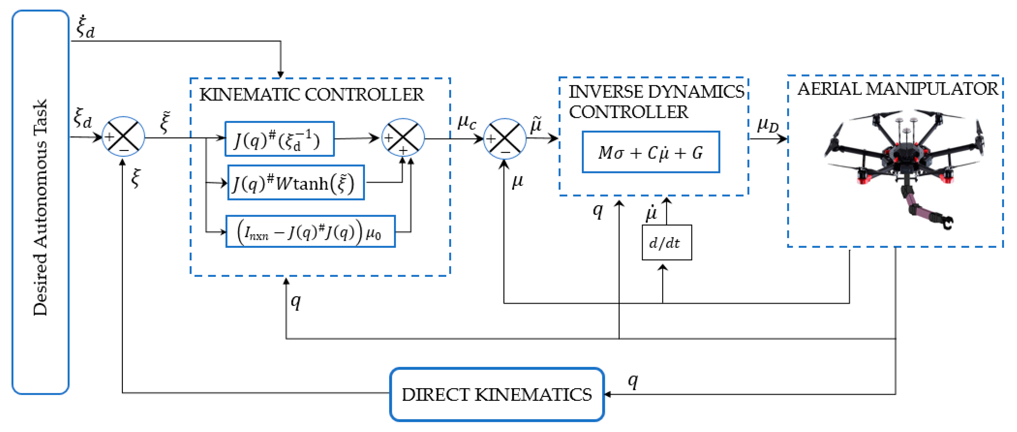
3.2. Inverse Dynamics Controller

The inverse dynamics controller is applied to systems with known dynamics, for which it is essential to obtain the system model and its dynamics be as close as possible to the real system so that it can be controlled. In addition, it is important to mention that it is not a robust controller because it depends directly on the changes that may exist in the dynamics of the system. The proposed controller scheme is shown in Figure 3.

The control law is given by:

$${\mu }_D\left(t\right)=M\left(q\left(t\right)\right)\sigma +C\left(q\left(t\right),\dot{q}\left(t\right)\right)\mu \left(t\right)+G\left(q\left(t\right)\right)$$

(13)

where ${\mu }_D(t)$ is the control action and σ is defined as:

$$\sigma ={\dot{\mu }}_c\left(t\right)+Q_{D}tanh\left( Q_D{}^{-1} K_D \tilde{\mu }\left(t\right)\right)$$

(14)

where ${\dot{\mu }}_c\left(t\right)$ is the derivative of the velocity of the Kinematic controller; $Q_D$ and $K_D$ are the positive definite calibration matrices; $\tilde{\mu }\left(t\right)={\mu }_c\left(t\right)-\mu \left(t\right)$ represents the velocity error; $\mu \left(t\right)$ is the velocity vector of the aerial manipulator robot, and ${\mu }_c\left(t\right)$ is the velocity vector of the Kinematic controller.

To analyze the stability of the controller, the system is considered in a closed loop, where it is established that $\dot{\mu }\left(t\right)=\sigma$ and replacing in Equation (14), we obtain:

$$0=\dot{\tilde{\mu }}\left(t\right)+Q_{D}tanh\left( Q_D{}^{-1} K_D \tilde{\mu }\left(t\right)\right)$$

(15)

From (15) it can be verified that $\tilde{\mu }\to 0$ When t → ∞.

3.3. Sliding Mode Controller (SMC)

The Sliding Mode algorithm considers the dynamics of a system that allows the fulfilment of the control objective by taking the system to a state space through a sliding surface, minimizing the disturbances that may occur. The scheme of this controller is shown in Figure 4.

The sliding surface s of the SMC is described below:

$$s={\lambda }_p\tilde{\mu }\left(\mathrm{t}\right)+{\lambda }_i{\displaystyle \int }\tilde{\mu }\left(\mathrm{t}\right) dt+{\lambda }_d \dot{\tilde{\mu }}\left(t\right)$$

(16)

Thus, $\tilde{\mu }\left(t\right)={\mu }_c\left(t\right)-\mu \left(t\right)$ is the error vector of velocities of the aerial manipulator robot; $\dot{\tilde{\mu }}\left(t\right)={\dot{\mu }}_c\left(t\right)-\dot{\mu }\left(t\right)$ is the derivative of the error with respect to time; ${\lambda }_p, {\lambda }_i$ y ${\lambda }_d$ is the positive definite calibration matrices of the proportional, integral, and derivative part of the controller, respectively.

Obtaining the first derivative of the surface (16) and replacing the errors calculated above, we obtain:

$$\dot{s}={\lambda }_p\left({\dot{\mu }}_c\left(t\right)-\dot{\mu }\left(t\right)\right)+{\lambda }_i\tilde{\mu }\left(t\right)+{\lambda }_d \ddot{\tilde{\mu }}\left(t\right)$$

(17)

where $\ddot{\tilde{\mu }}\left(t\right)$ is the second derivative of $\tilde{\mu }\left(t\right)$. The SMC control scheme is described with Equation (18)

$$u_{SMC}\left(t\right)=u_a\left(t\right)+u_d\left(t\right)$$

(18)

where $u_a\left(t\right)$. is the continuous part and $u_d\left(t\right)$ is the discontinuous part of the control action $u_{SMC}\left(t\right)$.

Considering $\dot{s}=0$ and $u_d\left(t\right)=0$ and replacing in Equation (17) we obtain:

$$u_a\left(t\right)=M\left(q\left(t\right)\right){\dot{\mu }}_c\left(t\right)+C\left(q\left(t\right),\dot{q}\left(t\right)\right) \mu \left(t\right)+G\left(q\left(t\right)\right)+M\left(q\left(t\right)\right){\lambda }_i{\lambda }_p{}^{-1}\tilde{\mu }\left(t\right)+M\left(q\left(t\right)\right){\lambda }_d{\lambda }_p{}^{-1} \ddot{\tilde{\mu }}\left(t\right)$$

(19)

Subsequently, the discontinuous part is determined by selecting the Lyapunov candidate $ℒ$ described in Equation (20), as a function of the area $s$.

$$ℒ=\frac{1}{2}{s}^{T}s$$

(20)

Deriving $ℒ$ with respect to time we obtain,

$$\dot{ℒ}=s^T\dot{s}$$

(21)

By replacing Equations (17) and (8) in Equation (21) and developing the expressions, we determine the derivative of $ℒ$.

$$\dot{ℒ}=s^T \left(-{\lambda }_p{\left(M\left(q\left(t\right)\right)\right)}^{-1}{u}_d\left(t\right)\right)$$

(22)

For Equation (22) to satisfy $\dot{ℒ}\le 0$, $u_d\left(t\right)$ is defined by:

$$u_d\left(t\right)=M\left(q\left(t\right)\right) k_2 sig\left(s\right)$$

(23)

where $k_2$ is a positive defined constant. By replacing Equation (23) in Equation (22) we obtain:

$$\dot{ℒ}=s^T \left(-{\lambda }_p k_2 sig\left(s\right)\right)$$

(24)

It is verified that if $k_2>0$ y ${\lambda }_d>0$, then $\dot{ℒ}<0$, therefore, $s\to 0$ with $t\to \infty$, hence, the error $\tilde{v}\to 0$ with $t\to \infty$. Then, the proposed controller is:

$$\begin{gathered} u_{SMC}\left(t\right)=M\left(q\left(t\right)\right){\dot{\mu }}_c\left(t\right)+C\left(q\left(t\right),\dot{q}\left(t\right)\right) \mu \left(t\right)+G\left(q\left(t\right)\right)+M\left(q\left(t\right)\right){\lambda }_i{\lambda }_p{}^{-1}\tilde{\mu }\left(t\right)+M\left(q\left(t\right)\right){\lambda }_d{\lambda }_p{}^{-1} \ddot{\tilde{\mu }}\left(t\right) \\ +M\left(q\left(t\right)\right)k_{2}sig\left(s\right) \end{gathered}$$

(25)

To improve the chattering condition, we propose that $k_2 sig\left(s\right) \cong \frac{s}{\left|s\right|+\delta }$ with $\delta >0$; finally, we obtain the control law given by:

$$u_{SMC}\left(t\right)=M\left(q\left(t\right)\right){\dot{\mu }}_c\left(t\right)+C\left(q\left(t\right),\dot{q}\left(t\right)\right) \mu \left(t\right)+G\left(q\left(t\right)\right)+M\left(q\left(t\right)\right){\lambda }_i{\lambda }_p{}^{-1}\tilde{\mu }\left(t\right)$$

$$+M\left(q\left(t\right)\right){\lambda }_d{\lambda }_p{}^{-1} \ddot{\tilde{\mu }}\left(t\right)+M\left(q\left(t\right)\right)k_2\frac{s}{\left|s\right|+\delta }$$

(26)

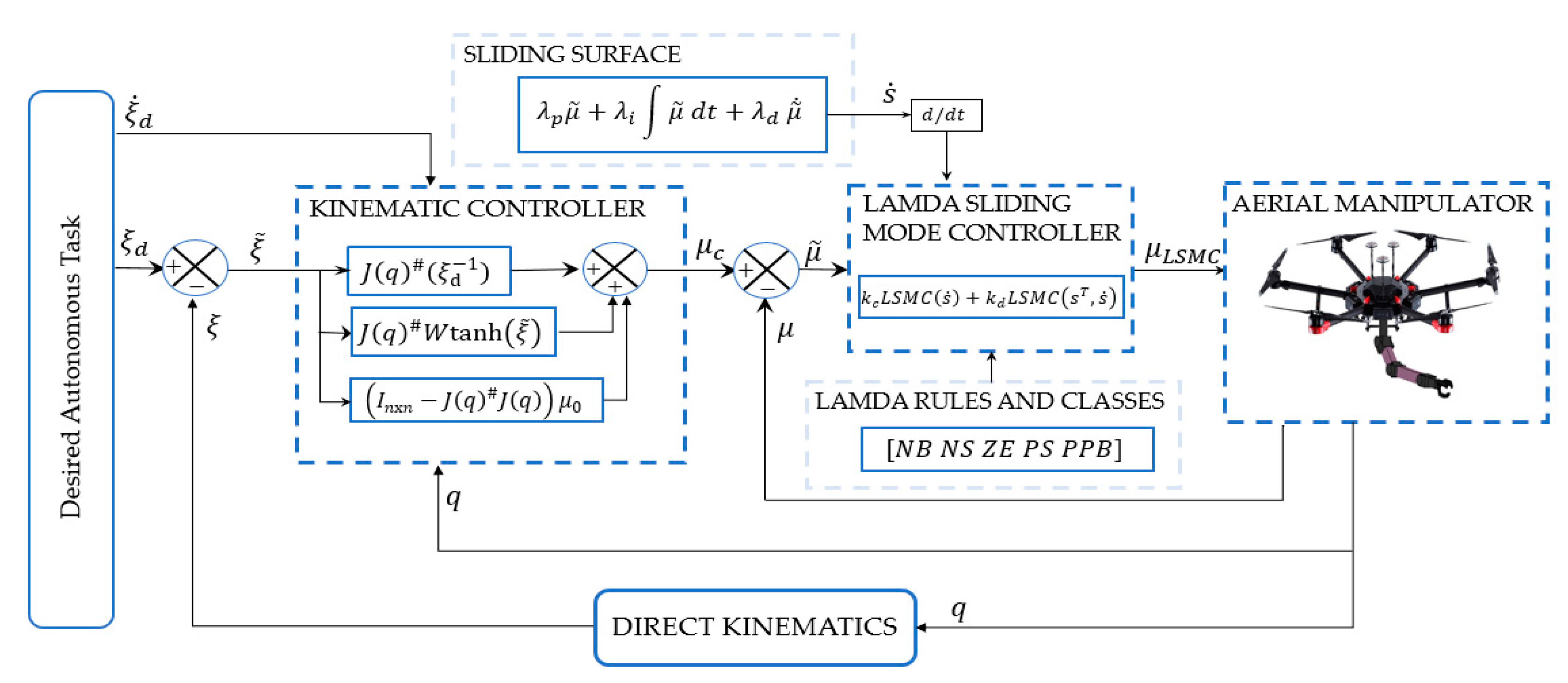
3.4. LAMDA Controller

The LSMC is an intelligent Sliding Mode controller based on LAMDA. The sliding surface defined in Equation (16) and its derivative defined in Equation (17) are composed of vectors with dimensions 7 × 1, therefore $s$ and $\dot{s}$. have the form: $s={\left[s_1 s_2\dots s_7 \right]}^T$ and $s={\left[{\dot{s}}_1 {\dot{s}}_2\dots {\dot{s}}_7 \right]}^T$.

The LAMDA controller (see Figure 5) is combined with the fundamentals of SMC for the calculation of continuous and discontinuous control actions [24]. For this purpose, the sliding surface $s_i$ and its derivative ${\dot{s}}_i$ are required, which describe an object $O_i$, such as: $O_i=\left[s_i {\dot{s}}_i\right]; \forall i=1,\cdots ,7,$ for all the variables to be controlled. The predefined classes $C=\left\{C_1;\cdots ; C_k; \cdots ; C_m\right\}$, are used to detect the current functional state of the system [23]. If we change the variables $s_1=o_{i1}$ and ${\dot{s}}_i=o_{i2}$, then the object $O_i$ is defined as:

$$O_i=\left[o_{i1} o_{i2}\right]$$

(27)

Now, the algorithm computes the Marginal Adequacy Degree (MAD), which is a parameter that measures the similarity of a descriptor with the same descriptor in a class using probability density functions, which require the average value of the descriptor j belonging to the class  (${\rho }_{k,ij}$) and its standard deviation set as ${\sigma }_{k,ij}=0.25$ [25].

$$MA{D}_{k,ij}=e^{-\frac{1}{2}{\left(\frac{o_{ij}-{\rho }_{k,ij}}{{\sigma }_{k,ij}}\right)}^2}$$

(28)

$${\rho }_{k,ij}=\frac{1}{n_{k,ij}}{{\displaystyle \sum }}_{t=1}^{n_{k,ij}}{o}_{ij}\left(t\right)$$

(29)

where $n_{k,ij}$ is the amount of data of the descriptor $ij$ in the class $k$.

The Global Adequacy (GAD) measures the membership degree of the object to each class and it is computed by mixing the MADs using fuzzy logic operators, and the Dombi operator [26] has been used in this work. The GADs are linear interpolations between the T-norm “$T\left(a,b\right)$” and the S-norm “$S\left(a,b\right)$” of the Dombi operator.

The parameters $a,b$ are the MADs in the class k to be operated with the T-norm and the S-norm, and $p\ge 1$ is used to modify the sensitivity.

The GAD for the object $O_i$ to each class $k$ is computed by the combination of T-norm and the S-norm as:

$$GA{D}_{k,O_i}\left(MA{D}_{k,i1},MA{D}_{k,i2}\right)=\alpha T\left(MA{D}_{k,i1},MA{D}_{k,i2}\right)+\left(1-\alpha \right)S\left(MA{D}_{k,i1},MA{D}_{k,i2}\right)$$

(30)

where $\alpha \in \left[0,1\right]$ is the exigency parameter. If $\alpha$ increases, then the algorithm is stricter, and if $\alpha$ decreases, then the algorithm is permissive.

The inference method presented in [24] proposes the use of LAMDA classes to evaluate the current state of the system and take corrective action to bring the system to the desired state. The analytical expression that describes the decision-making process is defined as:

$$R^{\left(k\right)}{}_i:IF o_{i1} is F_1^p and o_{i2} is F_j^q THEN y_{ki} is G_{ki}$$

(31)

where $R^{\left(k\right)}{}_i$ is the rule applied for the functional state (class) $k$, $o_{ij};\forall j=1,2$ is the descriptor $j$ of the object $O_i$ which takes on values of the universe of discourse $U_j$. The output linguistic variable $y_{ki}$ is defined on a universe of discourse $V$. $F_j=\left\{F_j^q:q=1,2,\dots ,Q\right\}$ is a fuzzy set on $U_j$ where $Q$ is the number of linguistic values and $G_{ki}$ is a fuzzy set on $V$.

The inference mechanism added to LAMDA is based on each GAD. The first-order TSK (Takagi-Sugeno-Kang) inference method [27] is employed, where $G_{ki}={\gamma }_{ki}.$ The parameter ${\gamma }_{ki}$ is a constant value specified for each class to bring the system to the desired functional state, which is $o_{i1}=0$ and $o_{i2}=0$. Then, the crisp output is computed as follows:

$$u_i={\zeta }_i{{\displaystyle \sum }}_{k=1}^m{\gamma }_{ki}GA{D}_{k,O_i}$$

(32)

where $u_i$ is the controller output for the object $O_i$, ${\gamma }_{ki}$ is its weight applied in the $k-\mathrm{th}$ rule, and ${\zeta }_i$ is the adjustment parameter for saturation of the output of the controller. The value of ${\zeta }_i$ is computed by:

$${\zeta }_i=\frac{\arg \max \left({\gamma }_{ki}\right)}{{{\displaystyle \sum }}_{k=1}^{m }{\gamma }_{ki}GA{D}_{k,argmax\left(O_i\right)}}$$

(33)

The procedure shown in Equations (27)–(33) is used to compute the control actions of for each variable (each controller). Now, to compute $u_{c_L}$ and $u_{d_L}$ of the SMC control action, the same surface defined in Equation (16) and its derivative defined in Equation (17) are used.

Replacing Equation (8) in Equation (17) we obtain:

$$\dot{s}={\lambda }_p\left({\dot{\mu }}_c\left(t\right)-{\left(M\left(q\left(t\right)\right)\right)}^{-1}\left[u_{c_L}-C\left(q\left(t\right),\dot{q}\left(t\right)\right)\mu \left(t\right)-G\left(q\left(t\right)\right)\right]\right)+{\lambda }_i\tilde{\mu }\left(t\right)+{\lambda }_d \ddot{\tilde{\mu }}\left(t\right)$$

$$\dot{s}={\lambda }_p\left({\dot{\mu }}_c\left(t\right)-{\left(M\left(q\left(t\right)\right)\right)}^{-1}{u}_{c_L}+{\left(M\left(q\left(t\right)\right)\right)}^{-1}C\left(q\left(t\right),\dot{q}\left(t\right)\right)\mu \left(t\right)-{\left(M\left(q\left(t\right)\right)\right)}^{-1}G\left(q\left(t\right)\right)\right)$$

$$+{\lambda }_i\tilde{\mu }\left(t\right)+{\lambda }_d \ddot{\tilde{\mu }}\left(t\right)$$

(34)

$M\left(q(t)\right)$ is defined as positive, thus, analyzing Equation (34), we can note that $\dot{s}$ decreases as $u_{c_L}$ Now, the algorithm computes the Marginal Adequacy Degree (MAD), which is a parameter that measures the similarity of a descriptor with the same descriptor in a class using probability density functions, which require the average value of the descriptor j belonging to the $\dot{s}=0$, which is the desired condition in SMC schemes.

The number of classes defined in each descriptor depends on the knowledge of the expert (designer). However, in the sensitivity analysis of Morales et al. [24], it is stated that with five classes per descriptor, very good results can be obtained without affecting the computational load. Thus, five classes are considered in this work $C\in \left[-1,1\right]$ for $\dot{s}$, as is detailed in [28]. The fuzzy sets for the classes of $\dot{s}$ are: Negative Big ($NB=-1$), Negative Small ($NS=-0.5$), zero ($ZE=0$), Positive Small ($PS=0.5$), and Positive Big ($PB=1$). These classes are used to define the rules to compute the normalized continuous control action $u_{n{c}_L}$. The scaling gain $k_{c_L}$ is used for tuning at the input $\dot{s}$, and the scaling gain $k_c$ at the output as:

$$u_{c_L}=k_{c_L}{u}_{n{c}_L} \Rightarrow u_{c_L}=k_{c}LSMC\left(\dot{s}\right); k_{c_L}>0$$

(35)

As a practical example, we can note that in Equation (35), if $\dot{s}$ is $PB$, then large positive control action $u_c$ is required to decrease quickly $\dot{s}$ in order to obtain $\dot{s}=0$. If $\dot{s}=ZE$, the desired condition is satisfied, then no control action is needed, thus $u_{c_L}=ZE$. The rule table corresponding to the continuous control action is shown in

Table 1. Rule table of LSMC for $\dot{s}$.

	$\dot{\mathit{s}}$
	NB	NS	ZE	PS	PB
M > 0	$$C_1=NB$$	$$C_2=NS$$	$$C_3=ZE$$	$$C_4=PS$$	$$C_5=PB$$

.

Consider that the values presented in Table 1 for each of the classes is the one corresponding to the weight applied to the control output ${\gamma }_k$.

To compute the discontinuous control action $u_{d_L}$, which is in charge of attracting the system to the sliding surface, we use the derivative of the Lyapunov function $\dot{ℒ}$ defined in Equation (21).

Replacing Equation (34) in Equation (21), and considering only the discontinuous control action u_LSMC = u_dL, we obtain:

$$s^T\dot{s}=s^T{\lambda }_p\left({\dot{\mu }}_c\left(t\right)-{\left(M\left(q\left(t\right)\right)\right)}^{-1}{u}_{a_L}+{\left(M\left(q\left(t\right)\right)\right)}^{-1}C\left(q\left(t\right),\dot{q}\left(t\right)\right)\mu \left(t\right)-{\left(M\left(q\left(t\right)\right)\right)}^{-1}G\left(q\left(t\right)\right)\right)$$

$$+s^T{\lambda }_i\tilde{\mu }\left(t\right)+s^T{\lambda }_d \ddot{\tilde{\mu }}\left(t\right)$$

(36)

To guarantee stability, Lyapunov theory establishes to satisfy the condition $\dot{ℒ}$< 0. Thus, considering Equation (36), it is necessary to satisfy $s^T\dot{s}$ < 0. As in the case of continuous control action, five classes are set for each input $\dot{s}$ and $s^T.$ Due to the normalization of the classes that is computed $u_{n{d}_L}$, the scaling gain $k_2$ is placed at the input $s$, and the scaling gain $k_d$ at the discontinuous control output as:

$$u_{d_L}=k_d{u}_{n{d}_L} \Rightarrow u_{d_L}=k_{d}LSMC\left(s^T,\dot{s}\right); k_d>0$$

(37)

The rule table for $u_{d_L}$ in which $\dot{s}$ and $s^T$ is required, considering that $M\left(q\left(t\right)\right)$ is defined positive, is shown in

Table 2. Rule table of LSMC for $s\left(t\right)$ and $\dot{s}$.

		$\dot{\mathit{s}}$
		NB	NS	ZE	PS	PB
ST	PB	C5 = ZE	C10 = ZE	C15 = PS	C20 = PB	C25 = PB
	PS	C4 = ZE	C9 = ZE	C14 = PS	C19 = PB	C24 = PB
	ZE	C3 = NB	C8 = NS	C13 = ZE	C18 = PS	C23 = PB
	NS	C2 = NB	C7 = NB	C12 = NS	C17 = ZE	C22 = ZE
	NB	C1 = NB	C6 = NB	C11 = NS	C16 = ZE	C21 = ZE

. The rule definition is detailed in [24].

Consider that the values presented in Table 2 for each of the classes are the ones corresponding to the weight applied to the control output ${\gamma }_k$. Table 2 can be analyzed as follows: For example, in the class $C_1,$ where $s^T=NB$ and $\dot{s}=NB$, the product $s^T\dot{s}$ is $PB$. Therefore, based on Equation (36) and when $s^T<0$, the negative control input is required $\left({\gamma }_1=NB\right)$ to quickly decrease $s\left(t\right)\dot{s}\left(t\right)$ The same situation is presented in the classes $C_2, C_6, C_7$. In the class $C_5,$ where $s^T=PB$ and $\dot{s}=NB$, the product $s^T\dot{s}$ is $NB$. Therefore, no change in the control action $u_d$ is required, thus ${\gamma }_5=ZE$. The other classes in which no change in the control action is required because the condition is met are $C_4, C_9, C_{10},$ $C_{16},$ $C_{17},$ $C_{21}$, and $C_{22}.$

As it can be seen in the controller, the $sig()$ function used in conventional SMC controllers (see Equation (23)) is not required, since LAMDA replaces this function, making it a chattering-free controller. The overall control action is represented in Figure 5, and defined as:

$$u_{LSMC}=k_{c}LSMC\left(\dot{s}\right)+k_{d}LSMC\left(s^T,\dot{s}\right)$$

(38)

where:

$$LSMC\left(\dot{s}\right)=\frac{\arg \max \left({\gamma }_{k1}\right)}{{{\displaystyle \sum }}_{k=1}^m{\gamma }_{k1}GA{D}_{k,argmax\left(O\right)}}{{\displaystyle \sum }}_{k=1}^m{\gamma }_{k1}GA{D}_{k,O } \mathrm{and};$$

$$LSMC\left(s^T,\dot{s}\right)=\frac{\arg \max \left({\gamma }_{k2}\right)}{{{\displaystyle \sum }}_{k=1}^{m }{\gamma }_{k2}GA{D}_{k,argmax\left(O\right)}}{{\displaystyle \sum }}_{k=1}^m{\gamma }_{k2}GA{D}_{k,O}$$

(39)

The stability of the controller is guaranteed if selected:

$$\left(k_c+k_d\right)>{\beta }_{vc}-\left({\beta }_A+{\beta }_d\right)$$

(40)

With:

$$\{\begin{array}{c}\Vert -{\left(M\left(q\left(t\right)\right)\right)}^{-1}C\left(q\left(t\right),\dot{q}\left(t\right)\right)\Vert \le {\beta }_A\\ \Vert {\dot{\mu }}_c\left(t\right)\Vert \le {\beta }_{v_c}\\ \Vert d\Vert \le {\beta }_d\end{array}$$

(41)

where β_vc, β_A, and β_d are the limits of the bounded functions corresponding to the change of the reference, the state matrix, and the disturbance, respectively. The expression (40) guarantees $\dot{ℒ}$ < 0, therefore, $s\to 0$ with $t\to \infty$ as proven in [26].

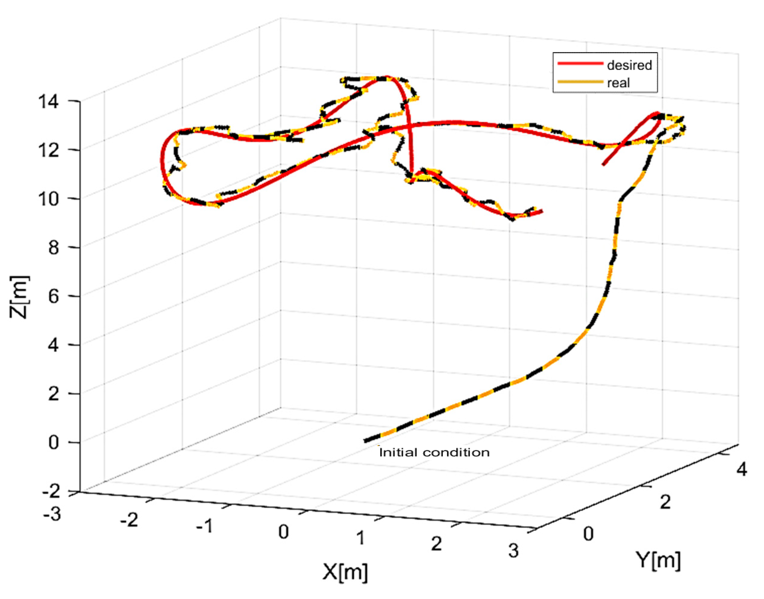
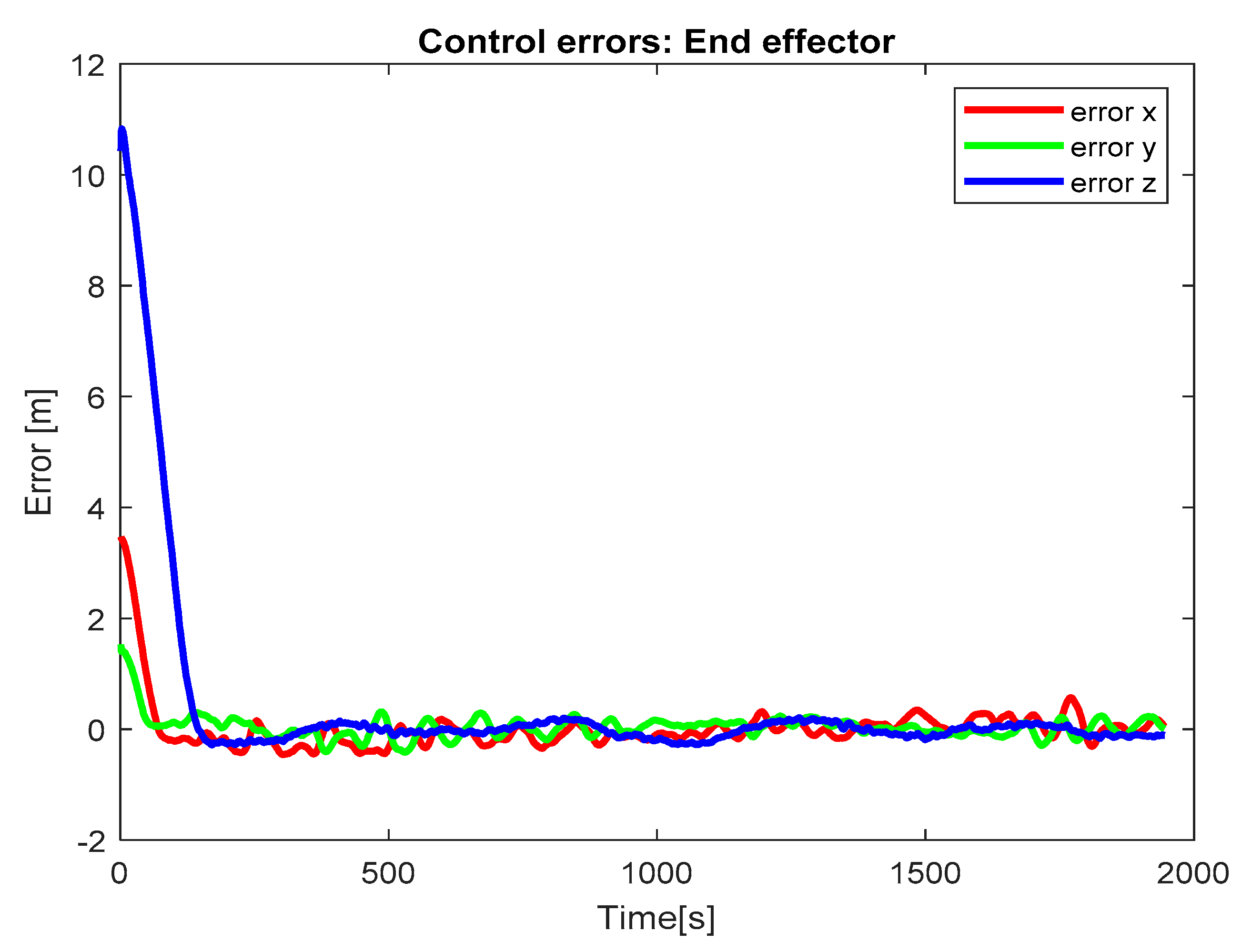
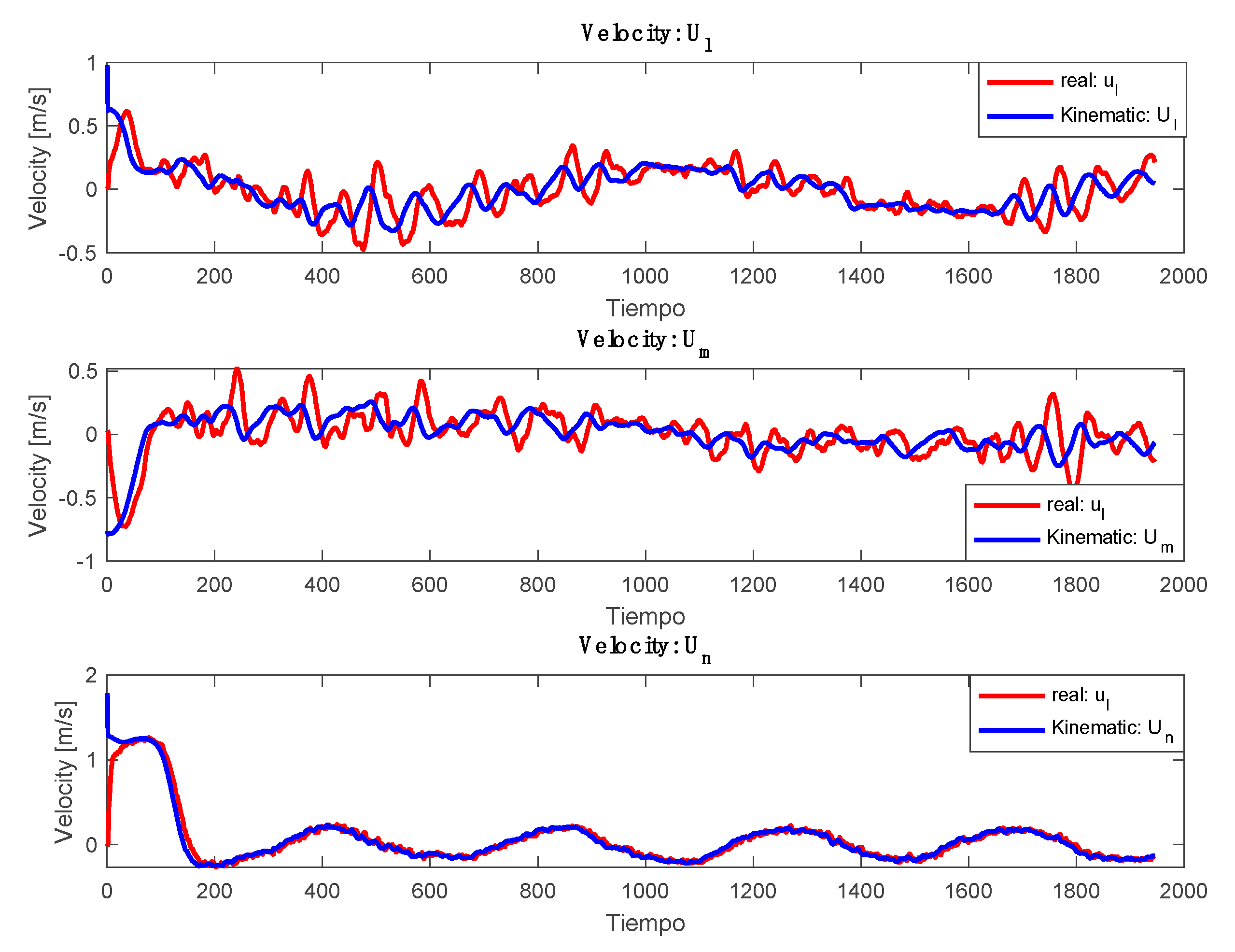
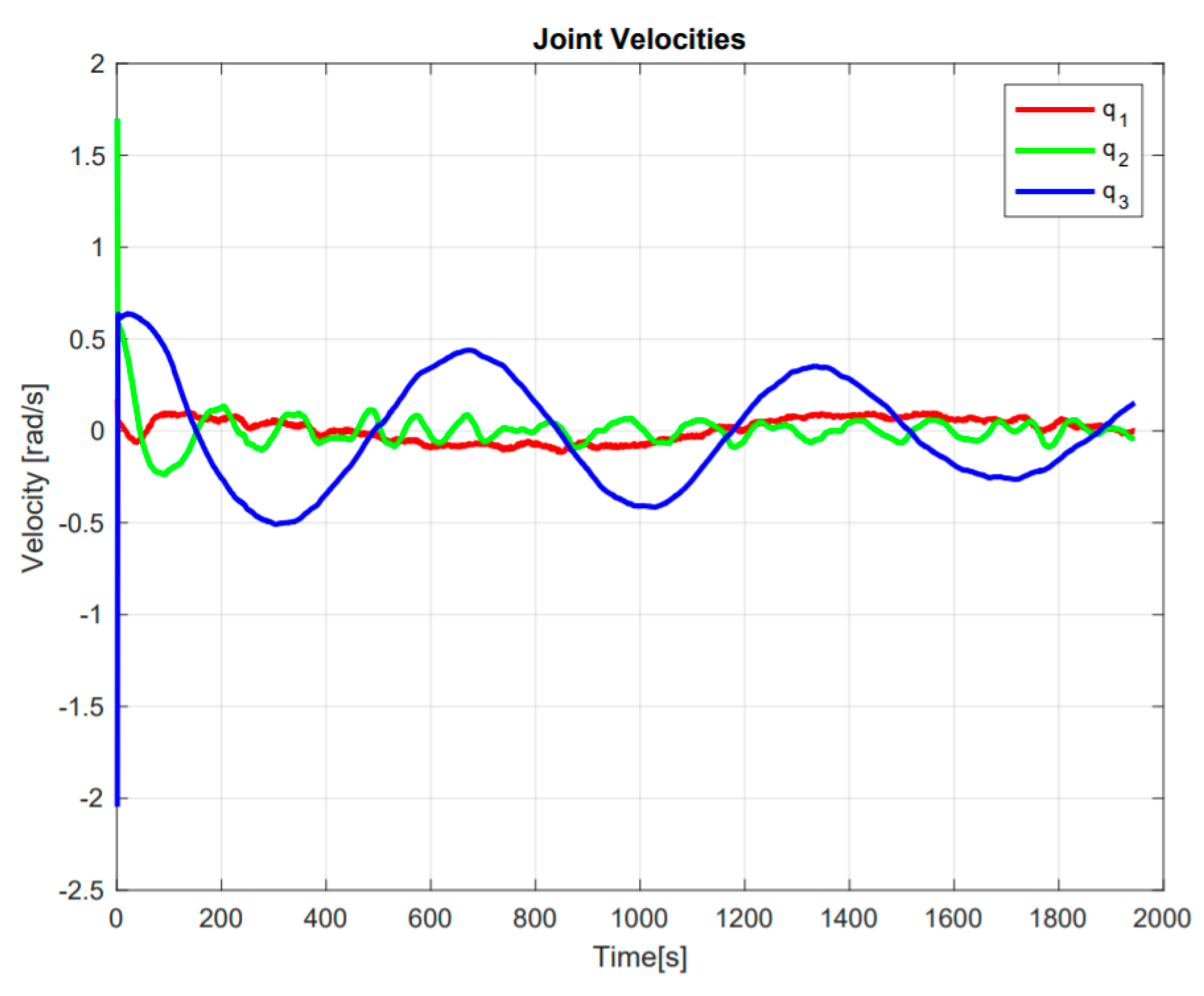
4. Experimental Results

This section presents the experimental results to validate the proposed control algorithms for the aerial manipulator robot. Four experiments are described on a real aerial manipulator robot with three degrees of freedom: (i) Experiment 1: Kinematic controller implementation, (ii) Experiment 2: Inverse Dynamics controller implementation, (iii) Experiment 3: SMC controller implementation, and (iv) Experiment 4: LAMDA controller implementation.

The tests consisted of the tracking of a lemniscate trajectory by the aerial manipulator robot, whose desired trajectory parameters were: ${\xi }_d=\left[{\xi }_{xd} {\xi }_{yd} {\xi }_{zd}\right]$, ${\xi }_{xd}=2.5\cos \left(0.02t\right)$ m, ${\mathsf{\xi }}_{\mathrm{yd}}=2.5\sin \left(0.04t\right)$ m, ${\mathsf{\xi }}_{\mathrm{zd}}=(\sin \left(0.1t\right)+0.6$) m. The time derivative of the desired trajectory was: ${\dot{\xi }}_d=\left[{\dot{\xi }}_{xd} {\dot{\xi }}_{yd} {\dot{\xi }}_{zd}\right]$, ${\dot{\xi }}_{xd}=\left(-2.5*0.2\sin \left(0.02t\right)\right)$ m/s, ${\dot{\xi }}_{yd}=(2.5*0.04cos\left(0.04t\right))$ m/s, ${ \mathsf{\xi } \dot{}}_{zd}=\left(0.1sin\left(0.1t\right)+12\right)$ m/s.

The parameters of the aerial manipulator robot were length of joints 1, 2, and 3 defined by $l_1=0.4$ m, l₂ = 0.26 m, $l_3=0.12$ m, and $r=0.12$ m, which is the height of the hexacopter. $q\left(t\right)=\left[ u_l u_m u_n \omega \dot{q_1} \dot{q_2} \dot{q_3}\right]=\left[ 0 0 0 0 0 0 0 0\right]$; $\left[q_{1_0} q_{2_0} q_{3_0}\right]=\left[0 0 0\right]°$. The initial conditions of position of the end-effector were $\xi =\left[-1.30-0.05 1.70\right]$ m and the initial conditions of position of the desired trajectory were ${\xi }_d{}_0 \left[2.5 2 12\right]$ m.

The following parameters were available in the kinematic controller: W = I_3x3 identity matrix, $K=I_{3x3}$ identity matrix, whereas the parameters defined for the Inverse Dynamics controller were: $K_D=I_{7x7}$ identity matrix, $Q_D=2I_{7x7}$ identity matrix. The SMC controller parameters were as follows: ${\lambda }_p=1;{\lambda }_d=1;{\lambda }_i=1; k_2=1; \delta =0.6$. Finally, the parameters of the LAMDA controller were stated as: k_c = 0.1I_7x7, $k_d={ℬ}_{7x7}$, a diagonal matrix whose diagonal elements are $\left[10 10 40 20 20 20 20\right]$, β_d = 0.5, ${\beta }_{vc}=0.1$, and ${\beta }_A=20$.

For the implementation of the four control algorithms, the experimental tests were carried out on the hexacopter-type aerial manipulator robot incorporating a three-degree-of-freedom robotic arm shown in Figure 6.

The experiments were developed in the city of Ambato, province of Tungurahua, Ecuador, whose latitude and longitude coordinates are 1°16′36.4″ S 78°35′19.0″ W. The experiment started at 14:32 on 20 February 2021. Wind velocity at that time and location was 8.3 km/h, approximately, according to [29] as evidenced in Figure 7.

4.1. Experiment 1: Kinematic Controller

In this experiment, the kinematic controller is implemented within the aerial manipulator robot to track the lemniscate trajectory. Figure 8 depicts the described trajectory, observing that there is an expected error in the tracking, due to the fact that the dynamics of the aerial manipulator robot had not been considered.

Figure 9 depicts the position errors obtained for the Kinematic controller, showing errors of up to 1 m of amplitude. These errors are because the dynamics of the aerial manipulator robot is not considered. In addition, the presence of wind influences the performance of the controller since it is considered as an external disturbance.

4.2. Experiment 2: Inverse Dynamics Controller

In this test, the performance of the controller for trajectory tracking is observed. The trajectory described by the aerial manipulator robot and the desired trajectory are presented in Figure 10. We observed that the end effector of the aerial manipulator robot follows the desired trajectory with a margin of error of approximately 0.4 m as verified in Figure 11. Therefore, a better performance of this controller is observed in comparison with the Kinematic controller, despite the presence of a wind of approximately 8.3 km/h.

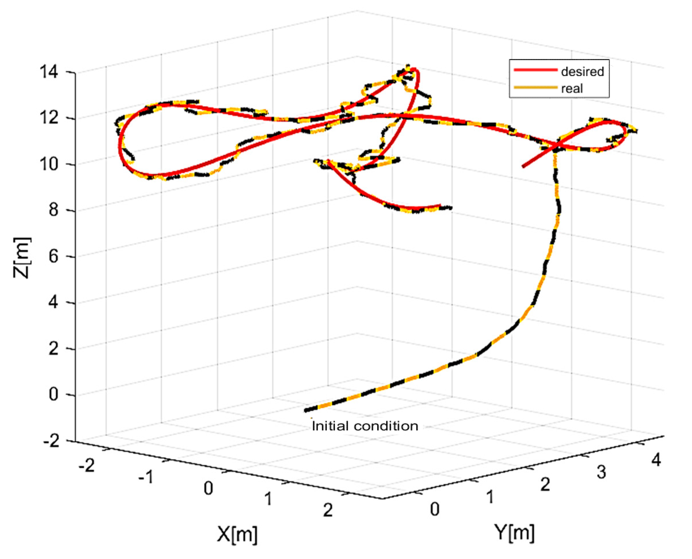
4.3. Experiment 3: SMC Controller

Figure 12 shows the results of the trajectory tracking performed by the aerial manipulator robot for this controller, showing that it performs a lemniscate trajectory with a margin of error similar to the Inverse Dynamics controller, since both controllers incorporate within their control law the compensation of the dynamics of the aerial manipulator robot. Figure 13 depicts the control errors present in this experiment, reaching a maximum value of approximately 0.4 m.

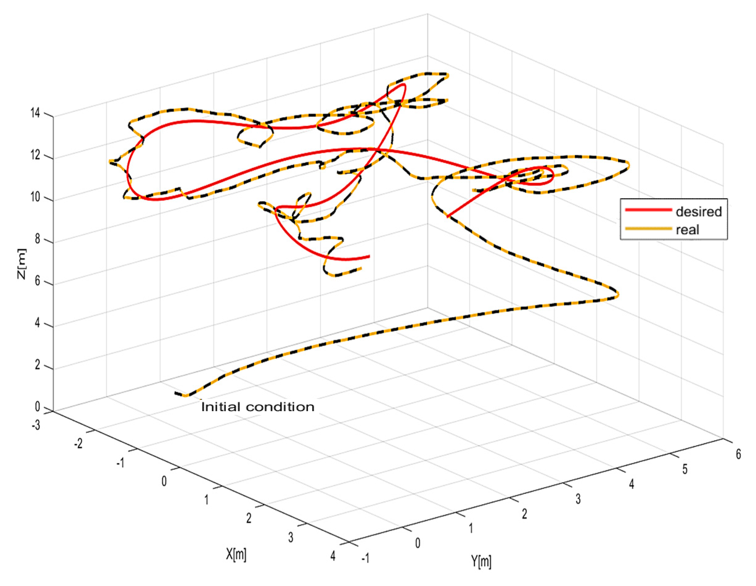
4.4. Experiment 4: LAMDA Controller

The results of the new control strategy applied for the trajectory tracking of an aerial manipulator robot are shown in Figure 14, Figure 15, Figure 16 and Figure 17. Figure 14 shows the trajectory carried out by the end-effector of the aerial manipulator robot, corroborating that it follows the desired trajectory with an expected margin of error.

Figure 15 shows the end-effector position errors, with a maximum error of approximately 0.4 m. This corroborates the good performance of the new proposed LAMDA control system that has not been used yet for aerial manipulators robots. This type of control even responds favorably to the presence of external disturbances such as wind velocity of approximately 8.3 km/h.

The control signals are shown in Figure 16, where we can observe that there is a good velocity tracking by the aerial manipulator robot, verifying that its control signals are smooth and slightly oscillatory, which allows its actuators to not receive abrupt signals that shorten its useful life.

The velocities of the joints of the robotic arm ${\dot{q}}_1, {\dot{q}}_2$ y ${\dot{q}}_3$ are shown in Figure 17. We observed that joint 3 generates an angular velocity greater than the rest of joints of robotic arm since it is easier for the aerial manipulator robot to move this joint of the robotic arm to achieve the control objective. Therefore, minor movements are generated in joint 1 and 2 as verified in this figure.

Taking into account the experiments carried out, it is possible to confirm the good behavior of the LAMDA controller, exhibiting a better performance compared to the Kinematic controller and a similar performance in comparison to the Inverse Dynamics and Sliding Mode control strategies for trajectory tracking.

The obtained Integral square error (ISE) factor is shown in Figure 18, verifying that the new LAMDA control proposal can be applied to aerial manipulators robots, obtaining a good performance that can be comparable to control techniques with dynamic compensation for these systems.

5. Discussion and Conclusions

In this work, experimental tests were carried out for four controllers: Kinematic, Inverse Dynamics, SMC Sliding Mode, and LAMDA, aimed at trajectory tracking by an aerial manipulator robot. The experimental results obtained from the Kinematic controller showed higher errors with respect to the other controllers. This fact was expected since the Kinematic controller does not compensate the dynamics of the system. Furthermore, the presence of wind causes the controller to not exhibit a good performance, as shown in Figure 18. The Inverse Dynamics, SMC, and LAMDA controllers exhibited better results with respect to the Kinematic controller, showing a good performance. The corresponding stability analysis of the proposed controllers have also been presented. The errors obtained in the latter controllers were as expected according to their nature. Furthermore, the presence of wind generates errors in the trajectory tracking.

The proposed LAMDA controller applied to trajectory tracking for the aerial manipulator robot demonstrated its stability in experimental tests under disturbance conditions. Therefore, the LAMDA controller shows a better performance than the Kinematic controller and a similar performance to the rest of the controllers developed in this work, as it can be seen in the experimental tests through the ISE.

Although LAMDA has similar results to the Inverse Dynamics and SMC controllers, its advantage over them is that LAMDA does not depend on the model of the aerial manipulator robot. Thus, it is not necessary to determine and obtain the parameters of the aerial manipulator robot for the implementation of the algorithm, which is usually complex and requires validation prior to use in the different control algorithms that are based on the model. Due to the nature of its structure, the LAMDA controller is based on a set of fixed hidden layers and is considered as an artificial intelligence method, whose computational performance is not as high compared to similar algorithms [24], as well as the fact that the mathematics turns out to be not so complex.

The LAMDA controller is a technique that has not been used previously for robotic systems such as aerial manipulators robots, although this type of controller has been implemented in other applications such as data analysis, data classification, system identification, and process regulation.

LAMDA is robust against disturbances due to its design based on the fundamentals of SMC, considering the stability of Lyapunov. LAMDA has presented good behavior in the presence of wind whose velocity was around 8.3 km/h, so there is evidence that promising results could be obtained with the application of this controller in the area of robotics, specifically for aerial manipulator robots.

The objective of this work is to demonstrate that the LAMDA controller was experimentally tested in applications not common to which it has been used habitually. Thus, for the first time, it has been used in aerial manipulators robots for trajectory tracking, the results of which confirm that LAMDA controllers can be brought into the field of robotics with promising results. Future work deals with the implementation of this controller for cooperative systems, as well as the application of adaptive fuzzy logic to the LAMDA controller to compensate systems with delays or disturbances that are usually present in robotic systems.

References

1. Tognon, M.; Chavez, H.A.T.; Gasparin, E.; Sable, Q.; Bicego, D.; Mallet, A.; Lany, M.; Santi, G.; Revaz, B.; Cortes, J.; et al. A Truly-Redundant Aerial Manipulator System with Application to Push-and-Slide Inspection in Industrial Plants. IEEE Robot. Autom. Lett. 2019, 4, 1846–1851. [Google Scholar] [CrossRef] [Green Version]
2. Hamaza, S.; Georgilas, I.; Richardson, T. 2D Contour Following with an Unmanned Aerial Manipulator: Towards Tactile-Based Aerial Navigation. In Proceedings of the 2019 IEEE/RSJ International Conference on Intelligent Robots and Systems (IROS), Macau, China, 4–8 November 2019; pp. 3664–3669. [Google Scholar]
3. Bartelds, T.; Capra, A.; Hamaza, S.; Stramigioli, S.; Fumagalli, M. Compliant Aerial Manipulators: Toward a New Generation of Aerial Robotic Workers. IEEE Robot. Autom. Lett. 2016, 1, 477–483. [Google Scholar] [CrossRef] [Green Version]
4. Lee, S.; Kim, H.; Kim, U.; Lee, H. Concave Wall Surface Tracking for Aerial Manipulator Using Contact Force Estimation Algorithm. In Proceedings of the 2020 20th International Conference on Control, Automation and Systems (ICCAS), Busan, Korea, 13 October 2020; pp. 850–855. [Google Scholar]
5. Yang, Y.; Liu, J.; Li, Z.; Yang, X.; Yu, X.; Gao, H. Nonlinear Disturbance Observer Based Adaptive Backstepping Control for Trajectory Tracking of Aerial Parallel Manipulator. In Proceedings of the IECON 2020 the 46th Annual Conference of the IEEE Industrial Electronics Society, Singapore, 18 October 2020; pp. 4776–4781. [Google Scholar]
6. Guayasamin, A.; Leica, P.; Herrera, M.; Camacho, O. Trajectory Tracking Control for Aerial Manipulator Based on Lyapunov and Sliding Mode Control. In Proceedings of the 2018 International Conference on Information Systems and Computer Science (INCISCOS), Quito, Ecuador, 14–16 November 2018; pp. 36–41. [Google Scholar]
7. Imanberdiyev, N.; Kayacan, E. Redundancy Resolution Based Trajectory Generation for Dual-Arm Aerial Manipulators via Online Model Predictive Control. In Proceedings of the IECON 2020 the 46th Annual Conference of the IEEE Industrial Electronics Society, Singapore, 18 October 2020; pp. 674–681. [Google Scholar]
8. Tlatelpa-Osorio, Y.E.; Rodriguez-Cortes, H.; Acosta, J.A. A Descentralized Approach for the Aerial Manipulator Trajectory Tracking. In Proceedings of the 2020 International Conference on Unmanned Aircraft Systems (ICUAS), Athens, Greece, 1–4 September 2020; pp. 504–511. [Google Scholar]
9. Wang, X.; Zhou, Z.; Chen, S.; Wang, R. Trajectory Tracking and Vibration Suppression of Spacecraft Combination Connected by a Space Manipulator. In Proceedings of the 2019 Chinese Control Conference (CCC), Guangzhou, China, 27–30 July 2019; pp. 8055–8060. [Google Scholar]
10. Camacho, O.; Leica, P.; Antamba, J.; Quinonez, J. Null-Space Based Control Applied to a Formation of Aerial Manipulators in Congested Environment. In Proceedings of the 2019 International Conference on Information Systems and Computer Science (INCISCOS), Quito, Ecuador, 20–22 November 2019; pp. 244–250. [Google Scholar]
11. Gkountas, K.; Tzes, A. Leader/Follower Force Control of Aerial Manipulators. IEEE Access 2021, 9, 17584–17595. [Google Scholar] [CrossRef]
12. Morton, K.; McFadyen, A.; Gonzalez, F. Generalized Trajectory Control for Tree-Structured Aerial Manipulators. In Proceedings of the 2018 International Conference on Unmanned Aircraft Systems (ICUAS), Dallas, TX, USA, 12–15 June 2018; pp. 947–956. [Google Scholar]
13. Jia, P.; Li, E.; Liang, Z.; Qiang, Y. Adaptive Neural Network Control of an Aerial Work Platform’s Arm. In Proceedings of the 10th World Congress on Intelligent Control and Automation, Beijing, China, 6–8 July 2012; pp. 3567–3570. [Google Scholar]
14. Muscio, G.; Pierri, F.; Trujillo, M.A.; Cataldi, E.; Antonelli, G.; Caccavale, F.; Viguria, A.; Chiaverini, S.; Ollero, A. Coordinated Control of Aerial Robotic Manipulators: Theory and Experiments. IEEE Trans. Contr. Syst. Technol. 2018, 26, 1406–1413. [Google Scholar] [CrossRef] [Green Version]
15. Liu, Y.-C.; Huang, C.-Y. DDPG-Based Adaptive Robust Tracking Control for Aerial Manipulators With Decoupling Approach. IEEE Trans. Cybern. 2021, 1–14. [Google Scholar] [CrossRef]
16. Naldi, R.; Pounds, P.; De Marco, S.; Marconi, L. Output Tracking for Quadrotor-Based Aerial Manipulators. In Proceedings of the 2015 American Control Conference (ACC), Chicago, IL, USA, 1–3 July 2015; pp. 1855–1860. [Google Scholar]
17. Mora-Florez, J.; Barrera-Nunez, V.; Carrillo-Caicedo, G. Fault Location in Power Distribution Systems Using a Learning Algorithm for Multivariable Data Analysis. IEEE Trans. Power Deliv. 2007, 22, 1715–1721. [Google Scholar] [CrossRef]
18. Botía Valderrama, J.F.; Botía Valderrama, D.J.L. On LAMDA Clustering Method Based on Typicality Degree and Intuitionistic Fuzzy Sets. Expert Syst. Appl. 2018, 107, 196–221. [Google Scholar] [CrossRef]
19. van der Tak, F.; Lique, F.; Faure, A.; Black, J.; van Dishoeck, E. The Leiden Atomic and Molecular Database (LAMDA): Current Status, Recent Updates, and Future Plans. Atoms 2020, 8, 15. [Google Scholar] [CrossRef]
20. Valderrama, J.F.B.; Valderrama, D.J.L.B. Two Cluster Validity Indices for the LAMDA Clustering Method. Appl. Soft Comput. 2020, 89, 106102. [Google Scholar] [CrossRef]
21. Ricardo Hernandez, H.; Luis Camas, J.; Medina, A.; Perez, M.; Veronique Le Lann, M. Fault Diagnosis by LAMDA methodology Applied to Drinking Water Plant. IEEE Latin Am. Trans. 2014, 12, 985–990. [Google Scholar] [CrossRef]
22. Morales Escobar, L.; Aguilar, J.; Garces-Jimenez, A.; Gutierrez De Mesa, J.A.; Gomez-Pulido, J.M. Advanced Fuzzy-Logic-Based Context-Driven Control for HVAC Management Systems in Buildings. IEEE Access 2020, 8, 16111–16126. [Google Scholar] [CrossRef]
23. Morales, L.; Aguilar, J.; Rosales, A.; Chávez, D.; Leica, P. Modeling and Control of Nonlinear Systems Using an Adaptive LAMDA Approach. Appl. Soft Comput. 2020, 95, 106571. [Google Scholar] [CrossRef]
24. Morales, L.; Aguilar, J.; Camacho, O.; Rosales, A. An Intelligent Sliding Mode Controller Based on LAMDA for a Class of SISO Uncertain Systems. Inf. Sci. 2021. [Google Scholar] [CrossRef]
25. Ruiz, F.A.; Isaza, C.V.; Agudelo, A.F.; Agudelo, J.R. A New Criterion to Validate and Improve the Classification Process of LAMDA Algorithm Applied to Diesel Engines. Eng. Appl. Artif. Intell. 2017, 60, 117–127. [Google Scholar] [CrossRef]
26. Morales, L.; Aguilar, J.; Chávez, D.; Isaza, C. LAMDA-HAD, an Extension to the LAMDA Classifier in the Context of Supervised Learning. Int. J. Inf. Technol. Decis. Mak. 2020, 19, 283–316. [Google Scholar] [CrossRef]
27. Wai, R.-J.; Chen, P.-C. Intelligent Tracking Control for Robot Manipulator Including Actuator Dynamics via TSK-Type Fuzzy Neural Network. IEEE Trans. Fuzzy Syst. 2004, 12, 552–559. [Google Scholar] [CrossRef]
28. Li, D.; Zhenqi, G. Trajectory Tracking Control of an Aerial Robot Based on Linear Active Disturbance Rejection Control Approach. In Proceedings of the 2019 Chinese Control And Decision Conference (CCDC), Nanchang, China, 3–5 June 2019; pp. 5004–5009. [Google Scholar]
29. Weather Spark. Average Wheather on February 20th in Ambato. 2021. Available online: https://es.weatherspark.com/d/20027/2/20/Tiempo-promedio-el-20-de-febrero-en-Ambato-Ecuador#Sections-Wind (accessed on 25 March 2021).
Figure 1. Aerial manipulator robot schematic.
Applsci 11 05885 g001
Figure 2. Proposed controller scheme.
Applsci 11 05885 g002
Figure 3. Proposed inverse dynamics controller scheme.
Applsci 11 05885 g003
Figure 4. Sliding Mode Controller scheme.
Applsci 11 05885 g004
Figure 5. LSMC controller scheme.
Applsci 11 05885 g005
Figure 6. Aerial manipulator robot used in the in experimentation.
Applsci 11 05885 g006
Figure 7. Wind velocity during experimentation.
Applsci 11 05885 g007
Figure 8. Trajectory tracking: Kinematic controller.
Applsci 11 05885 g008
Figure 9. Control errors: Kinematic controller.
Applsci 11 05885 g009
Figure 10. Trajectory tracking: Inverse Dynamics controller.
Applsci 11 05885 g010
Figure 11. Control errors: Inverse Dynamics controller.
Applsci 11 05885 g011
Figure 12. Trajectory tracking: SMC controller.
Applsci 11 05885 g012
Figure 13. Control errors: SMC controller.
Applsci 11 05885 g013
Figure 14. Trajectory tracking: LAMDA controller.
Applsci 11 05885 g014
Figure 15. Control errors: LAMDA controller.
Applsci 11 05885 g015
Figure 16. Control signals: LAMDA controller.
Applsci 11 05885 g016
Figure 17. Joint velocities: LAMDA controller.
Applsci 11 05885 g017
Figure 18. ISE factor for the different control techniques used in the experiments.
Applsci 11 05885 g018