PV Fault Detection Using Positive Unlabeled Learning

Abstract

Solar array management and photovoltaic (PV) fault detection is critical for optimal and robust performance of solar plants. PV faults cause substantial power reduction along with health and fire hazards. Traditional machine learning solutions require large, labeled datasets which are often expensive and/or difficult to obtain. This data can be location and sensor specific, noisy, and resource intensive. In this paper, we develop and demonstrate new semi supervised solutions for PV fault detection. More specifically, we demonstrate that a little-known area of semi-supervised machine learning called positive unlabeled learning can effectively learn solar fault detection models using only a fraction of the labeled data required by traditional techniques. We further introduce a new feedback enhanced positive unlabeled learning algorithm that can increase model accuracy and performance in situations such as solar fault detection when few sensor features are available. Using these algorithms, we create a positive unlabeled solar fault detection model that can match and even exceed the performance of a fully supervised fault classifier using only 5% of the total labeled data.

1. Introduction

Photovoltaic (PV) solar array faults including soilage, shading, degradation, and short circuit faults can reduce solar array power efficiency by an estimated 22.34% to 27.58% [1]. Several machine learning (ML) methods have been studied for solar fault detection, with most modern algorithms using some type of deep neural network solution [2,3,4,5] provide a thorough survey of current algorithms in the field and results are promising, however training the current state of the art deep learning algorithms is quite data intensive and requires large, labeled data sets. Collecting and labeling these large datasets is expensive and the data may be unique and sometimes must be at least partially re-collected for each PV solar array and location. In this paper, we develop and demonstrate a new fault detection algorithm that requires significantly less labeled training samples using positive and unlabeled learning (PU learning)—a family of newer semi-supervised positive unlabeled learning algorithms that has never, to our knowledge, previously been applied to PV fault detection. General semi-supervised learning algorithms use some labeled data but improve their models with additional unlabeled data [6]. In recent years, some semi-supervised algorithms have been applied to PV fault detection [7,8,9,10] for the very reasons listed above. However, general semi-supervised learning algorithms require some labeled data from both the positive (in this case the solar fault) class and the negative (clean, non-faulty) class. PU learning is a binary semi-supervised classification process in which only a small quantity of labeled data from only one class (the positive class) is available, along with a quantity of inexpensive and unlabeled data [11,12]. This is useful as while PV faults may be noticeable, care must be taken not to miss a fault before declaring a datapoint as fault-free.

We start by adapting an existing algorithm called the modified logistic regression (MLR) PU learning algorithm developed by the authors of this paper [13] for use in solar fault detection and similar problems. The resulting new algorithm is called the Feedback enhanced MLR (MLRf) algorithm and was designed for solar fault classification and related PU learning problems where there are limited features and labeled data. We compare these and other solar fault detection algorithms using the standardized NREL PVWatts [4,14] solar fault dataset (described later in this paper) for insight into the fault classification problem and to determine the number of labeled data required for effective solar fault classification. For each algorithm, excluding the oracle (a supervised learning algorithm that knows all and sees all—typically used as a best-case comparator), the percentage of known, labeled fault data is varied between 2% and 90% of the total positive data.

Solar fault detection algorithms compared in this paper (and explained in more depth in Section 2) include:

(1)

The MLR algorithm described in [13].

(2)

The MLRf algorithm proposed and described in this paper.

(3)

A naïve PU implementation using a supervised learning algorithm and treating all unlabeled datapoints as negatives.

(4)

An “oracle” supervised learning algorithm with all labels known.

(5)

A “tiny” supervised learning algorithm (we used the term “tiny”, not to indicate a specific algorithm, but to indicate the process where the training is done with a small number of labels. Not to be confused with Tiny ML algorithms.) using the same number of labeled data as MLR or MLRf, but in this case balanced between positive and negative samples instead of only positive.

(6)

An unsupervised kmeans clustering algorithm, mostly for curiosity and to illustrate the benefit of having some labels in all other cases.

We found that the PU learning algorithms, both the existing MLR and the new MLRf, were able to match and even outperform even the fully supervised oracle algorithm with only 5% of the data labeled. We additionally demonstrate that using the same number of labeled samples, the PU learning algorithms both outperform a smaller supervised learning algorithm that does not take advantage of the unlabeled samples. This, in addition to the fact that it is the nature of the problem that it is easier to label a faulty sample than to guarantee that a sample is not faulty, confirms that given a labeling budget, it is more effective to label only faulty samples than to attempt to label both faulty and non-faulty ones.

The main contributions of this paper are: (1) the use of a unique PU learning algorithm for solar array fault detection which has, to our knowledge, never been done before, (2) the adaptation of the MLR to work for solar fault detection, (3) the ability to effectively use significantly fewer labeled training data than most supervised learning algorithms by applying PU learning techniques to solar fault detection problems, (4) the introduction of a new PU learning algorithm, MLRf, designed to better detect and classify solar fault data, (5) the development of new comparative results demonstrating the effectiveness and robustness of the MLR and MLRf algorithms at detecting solar faults with very little labeled data, and (6) the demonstration that labeling $x$ positive samples is more effective than labeling $x$ total positive and negative samples. The novelty of this work lies most especially in the application of PU learning algorithms to solar fault detection and to the introduction of the MLRf algorithm.

2. Materials and Methods

In this section we describe the NREL PVWatts [4,14] solar fault dataset that we use in our experiments as well as a more detailed description of the new or unusual algorithms from the introduction: the MLR [13], MLRf, naïve PU, oracle, and “tiny” supervised learning algorithms.

But first, a quick note on notation. In addition to the standard classification notation of using $\overline{x}$ and $y$ to represent a data sample and its label respectively, a new random variable $s$ is introduced to represent if that sample is labeled or unlabeled. The PU problem can then be formally stated as:

$$p(s=1 | y=0)=0$$

(1)

Our classification goal can be thought of as the creation of a probabilistic function $f\left(\overline{x}\right)$ such that

$$f\left(\overline{x}\right)=p(y=1 | \overline{x})$$

(2)

2.1. Dataset

For this study, a solar fault dataset described in [4] was used, derived, and modified from data generated by the PVWatts calculator at the National Renewable Energy Laboratory (NREL) [14]. The dataset contains 21,485 solar measurements including equal parts (of 4297 each) clean, “no fault” or “standard conditions” data (STC), shaded, soiled, degraded, and short circuit solar data. Each measurement has ten features—the DC output, the open circuit voltage ($V_{OC}$), short circuit current ($I_{SC}$), max power point voltage ($V_{mp}$), max current ($I_{MP}$), fill factor, temperature, irradiance, gamma ratio, and max power. The dataset was labeled based on these feature measurements as described in [4]. A measurement was considered no fault or STC if the irradiance, temperature, and power were at the maximum values for that day. Data was labeled shaded if the measured irradiance was lower than the STC by 25% or more. Soilage was labeled as present if the irradiance was high while the power was low, while a short circuit was identified when the irradiance and temperature were standard but the maximum current, ($I_{MP}$), was low. A solar panel was labeled as degraded if the open circuit voltage, ($V_{OC}$), or short circuit current, ($I_{SC}$), were more than 25% below the rating of the PV module.

2.2. The MLR Algorithm

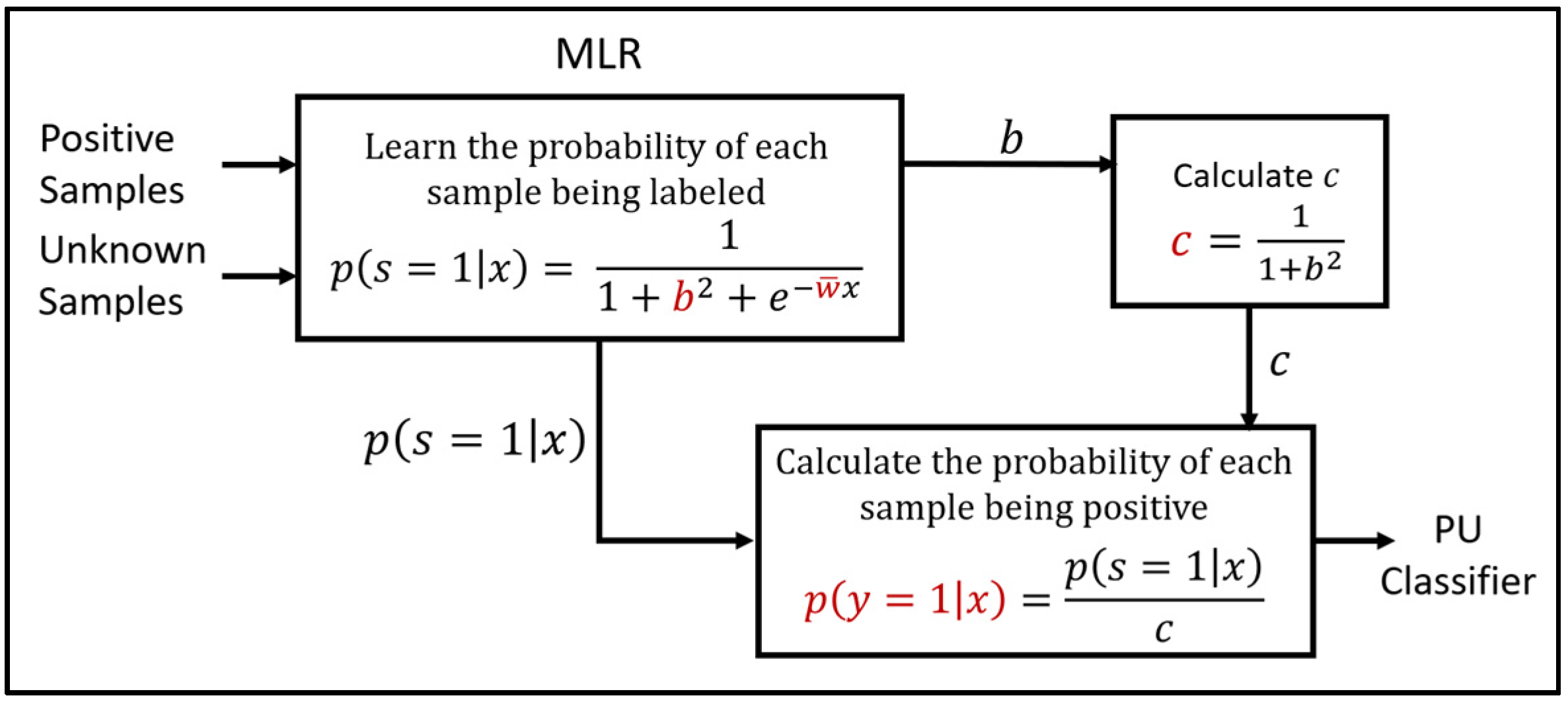
While the MLR algorithm is described in detail in [13], we will provide a summary here for clarity. As first described and proved in the foundational positive unlabeled learning paper [15], if we make a strong, but common assumption called the SCAR assumption and assume that the labeled positive (fault) data is selected at random from the set of all positive (fault) data, then we can create a non-traditional classifier $g\left(\overline{x}\right)=p(s=1|\overline{x})$ that can be used to obtain our final PU classifier $f\left(\overline{x}\right)$. By assuming that the labeled positive data is selected at random from all positive data, the probability of being labeled is no longer dependent on the feature vector $\overline{x}$, but only on the sample’s positive status $y=1$ as shown in Equation (3). This results in a constant labeling frequency named $c$ in the literature:

$$SCAR assumption:p(s=1| \overline{x}, y=1)=p(s=1|y=1)=c$$

(3)

This final PU classifier based on a non-traditional classifier is derived in [15] and reproduced as follows:

$$\begin{gathered} g\left(\overline{x}\right)=p(s=1| \overline{x})=p(s=1\wedge y=1| \overline{x}) \\ =p\left(y=1 | \overline{x}\right) p\left(s=1|y=1,\overline{x}\right) \\ =p\left(y=1|\overline{x}\right) p(s=1|y=1) \\ =p\left(y=1|\overline{x}\right) c. \end{gathered}$$

(4)

therefore:

$$f\left(\overline{x}\right)=p\left(y=1|\overline{x}\right)=\frac{p\left(s=1|\overline{x}\right)}{c}$$

(5)

In [13], we were able to demonstrate using both real-world and simulated datasets that the modified logistic regression (MLR) algorithm was an effective non-traditional classifier and produced better estimates of both $s$ and $y$ than existing algorithms. The MLR is defined by the expression:

$$MLR=p(s=1|\overline{x})=\frac{1}{1+b^2+e^{-\overline{\omega }·\overline{x}}}$$

(6)

where $b$ and $\overline{\omega }$ are variables that are learned in the training process. From this MLR algorithm and its learned parameter $b$, we are able to estimate the label frequency $c$ as the upper asymptote of Equation (6) as:

$$c=\frac{1}{1+b^2}$$

(7)

and from this construct a final PU classifier $f\left(\overline{x}\right)$ using Equation (6). After all data values have been mean normalized, a stochastic gradient ascent algorithm is used to maximize the likelihood of the MLR. The MLR algorithm details and block diagram are available in Appendix A Algorithm A1 and Figure A1.

The MLR algorithm provides an effective, general purpose PU learning algorithm, but like traditional logistic regression, on which it is based, the model it creates it is mostly linear in terms of the feature values of the inputs. When the feature set is small, additional feature engineering and enhancement is useful.

2.3. The MLRf Algorithm

PV fault detection and classification are different from typical classification problems as the feature set is typically small, while vast quantities of unlabeled data can be generated automatically. Our dataset has thousands of measurements but only 10 features, and some of those features such as the gamma ratio are calculated as combinations of other features.

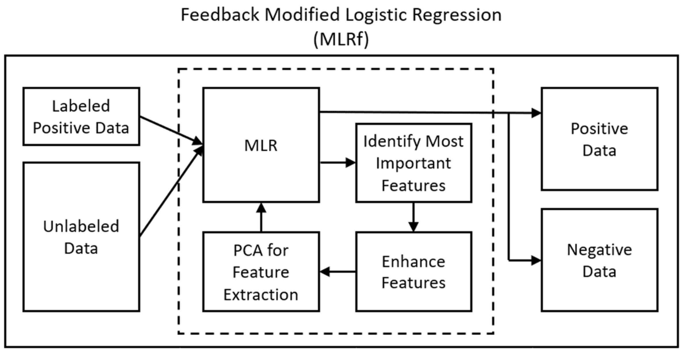
Because our feature set is small and the problem complex, linear classifiers may underfit the data, yet because a PU dataset has many missing labels, most non-PU non-linear classifiers such as neural networks will overfit the data to the few labeled datapoints. The MLR algorithm by itself is a powerful general-purpose PU learning algorithm, analogous to standard classification algorithms such as logistic regression, support vector machines, or artificial neural networks for fully labeled data and by itself includes no feature enhancement or engineering. To better handle the small solar fault detection feature set, we introduce the MLRf algorithm in this paper. The MLRf algorithm shown in Figure 1 uses the MLR algorithm, but also incorporates a feedback loop to perform custom feature engineering—enhancing the feature set to enable non-linear classification that does not overfit or underfit the data. This automates some of the preprocessing steps that are manually required by other algorithms.

The proposed MLRf algorithm consists of the following five steps.

(1)

An initial classification model is learned using the original MLR algorithm from [13] and described in Section 2.2.

(2)

The MLR model produced in Step 1 above is a weighted combination of $n$ feature variables. As the original feature data were mean normalized as part of training, the most influential features in the model are those with the highest magnitude weights. This allows us to sort the features by importance to the model. The MLRf algorithm selects the top $k\le n$ most important features by magnitude for enhancement.

(3)

Feature enhancement is performed by adding $p$-level polynomial combinations of the selected features. For example, if $p=2$ an enhancement of any two pairs of original features $x_1$ and $x_2$ would return the enhanced feature space $x_1,x_1^2, x_2, x_2^2, \mathrm{and} x_1·x_2$. If $p=3$, enhancement would include cubic values and combinations such as $x_1·x_2·x_3$, and so forth. The purpose of this expansion is to increase the dimensionality of the dataset to allow for a more flexible non-linear decision boundary that is better able to accommodate the complexity of the solar fault data space. A linear decision boundary in this higher dimensional space is equivalent to a non-linear decision boundary in the original feature space.

(4)

Once the feature space has been expanded, regularization methods or additional feature manipulation can be performed using a dimensionality reduction algorithm such as PCA (Principal Component Analysis) to capture the dimensionality of the enhanced feature set that incorporates more than 95–99% of the variability of the space. This eliminates or minimizes any enhanced features that do not substantially contribute to the final classification.

(5)

Finally, the newly expanded feature space is sent back through the original MLR classifier for final classification with a now potentially non-linear classification boundary.

In addition to the standard hyperparameters such as the learning rate and number of epochs in the MLR algorithm, the MLRf introduces $k$, the number or percentage of important features to be enhanced, and $p$, the level of polynomial enhancement described in step 2 above. If PCA is used in step 4, then the number of retained components becomes an additional hyperparameter. Regularization may be preferred for this reason. Once the model has been created, it can be applied to new data in real time. To capture possible changing conditions, offline training and model updates can be performed periodically.

2.4. The Naïve PU Algorithm

In practice, data with no detected faults is often labeled as negative, or not faulty. This strategy is replicated in this naïve PU algorithm which treats all unlabeled data samples as negative and performs a standard supervised classification (in this case a traditional logistic regression).

2.5. The Oracle

In computer science, an oracle is the name given to an algorithm that “knows all and sees all”. In the context of this semi-supervised learning algorithm, an oracle is a fully supervised learning algorithm that has access to all the true data labels. As the two algorithms of interest, MLR and MLRf, are both fundamentally related to the traditional logistic regression algorithm, the oracle algorithm (and indeed all other comparative algorithms) use traditional, or standard logistic regression (SLR) in this paper to provide a better measure of comparison. In all algorithms but k-means, a simple unoptimized stochastic gradient ascent algorithm was used to fit the data. We recognize that it is likely that other more complex supervised learning algorithms or other more advanced solvers could improve these algorithm’s performance, but our objective in this paper is to assess the MLR and MLRf algorithms against others in their same class. As these algorithms are still being researched and have not yet been optimized, we compare them to algorithms created in a similar manner. It is likely that with optimization (regularization, batch processing, more complex solvers, and so on) that eventual results will be substantially higher than they are now.

2.6. The “Tiny” Supervised Learning Algorithm

To compare the effect of having a small labeling budget more equitably, we create this supervised learning algorithm that only trains with the same number of data points that the MLR and MLRf algorithm have labeled. If MLR and MLRf have $x_L$ positive labeled and $x_{UL}$ samples available to them, this “tiny” supervised learning algorithm has $x_L$ total samples available—half positive and half negative. No unlabeled data is used. This is intended to simulate an assumed preference for supervised learning given a limited labeling budget and to compare this with the PU learning algorithm.

2.7. The K-Means Algorithm

We include in our algorithm comparison a simple unsupervised learning algorithm, more as a matter of curiosity than as a true comparison with the MLR and MLRf algorithms. K-means was performed using $\mathrm{k}=5$ clusters representing the five known classes in the data: shaded, soiled, degraded, short circuit, and no faults. After clustering, the individual cluster, or clusters (when performing general fault classification), were chosen to be labeled positive that contained the most samples belonging to the PU labeled positive class.

3. Results

3.1. Experimental Setup

To test our model, we compared each fault type (shaded, soiled, degraded, and short circuit—abbreviated SC) individually against all other data, including the other fault data and the non-fault STC data. We also grouped all fault data together into a single “fault” class that we compared against non-fault STC data. This latter is equivalent to a general fault detection, while the former enables specific fault classification were such information known. These details are illustrated in

Table 1. The binary composition of the five compared fault types.

Name	Positive Fault Data	Size of Positive Set	Negative Non-Fault Data	Size of Negative Set
All Faults vs. No Faults	Shaded, Soiled, Degraded, SC	17,188	STC	4297
Shaded vs. All Others	Shaded	4297	STC, Soiled, Degraded, SC	17,188
Soiled vs. All Others	Soiled	4297	STC, Shaded, Degraded, SC	17,188
Degraded vs. All Others	Degraded	4297	STC, Shaded, Soiled, SC	17,188
Short Circuit vs. All Others	SC	4297	STC, Shaded, Soiled, Degraded	17,188

.

For each of the above listed five fault types, we selected random subsets composed of different percentages between $c=2\%$ and $90\%$ of the true positive fault data to be labeled positive out of the original. The label frequency $c$ is unknown in a real PU dataset and constructed in simulated PU datasets such as this for algorithm evaluation. Using standard classification notation with $\overline{x}$ representing a data sample, this label frequency is defined as:

$$c=p(s=1 | y=1).$$

(8)

As some papers in the PU learning field use the class prior rather than the label frequency $c$, we provide a simple translation:

$$class prior=p\left(y=1\right)=\frac{p\left(s=1\right)}{c}.$$

(9)

To reduce variability, each experiment listed above was run five times and the mean evaluation metrics reported for each $c$ value in the graphs shown in Section 3.4. This is described in more depth in Section 3.3.

3.2. Hyperparameter Selection

The hyperparameters associated with the MLRf algorithm are the learning rate, the number of epochs, the percentage of features to enhance $k$, the level of enhancement $p$, and the level of PCA feature extraction, if used. Hyperparameter tuning was performed using a grid search looking first at the learning rate and number of epochs over the MLR algorithm with no $p$ or $k$. We found that a learning rate of 0.01 and 1000 epochs generally provided the best results. A further grid hyperparameter search investigated the percentage of important features to be enhanced $k=0.3, 0.6,$or 1 (MLRf step 2), the values of the polynomial expansion variable $p=1, 2, 3, 4$ (MLRf step 3), and the PCA level of feature extraction (MLRf step 4). We found that while the optimal $k$ values differed for each fault type, the polynomial expansion level of $p=3$ combined with no PCA feature reduction gave the best results across all faults. Adding in regularization, which was not implemented in these experiments, would potentially be beneficial in the future. General fault detection and identifying solar panel soilage performed best when $k=0.3$; short circuit faults were best detected when $k=0.6$; the remaining faults were most effective when $k=1$.

3.3. Evaluation Metrics

In PU learning in general it is common to have heavily skewed datasets with the rare class generally labeled positive. With only a fraction of the rare positive class labeled, PU classification is a skewed classification problem with too few data to perform class balancing measures. Instead, the F-score (also called the f1-score) is typically used to evaluate each experiment as the accuracy and error rate metrics are misleading when the class sizes are not similar (if 99% of the data were negative and 1% positive, a model that predicts everything negative would have a 99% accuracy and be completely worthless). The F-score is the harmonic mean between the precision and recall (also known as sensitivity). The F-score can be thought of as analogous to accuracy in that it varies between zero and one, with better models being closer to one. The F-score is calculated as:

$$Fscore=2·\frac{Precision·Recall}{Precision+Recall}$$

(10)

where:

$$Precision=\frac{\# True Positives}{\# True Positives+\# False Positives}$$

(11)

and:

$$Recall=\frac{\# True Positives}{\# True Positives+\# False Negatives}.$$

(12)

For each fault type and $c$ value, the MLRf algorithm was run five times and the mean value was chosen as the F-score. This was intended to reduce variance, though we found that the variance per run was minimal when $c$ was greater than 10%. High variance with small $c$ values is not unexpected as the random selection of the labeled samples becomes more impactful as the number of samples decrease. Tables including these mean and variance values are available in

Table A1. This table provides the raw results for Figure 2 and their variance.

		All Faults vs. No Faults		Shaded vs. All Others		Soiled vs. All Others		Degraded vs. All Others		Short Circuit vs. All Others
MLR	c	F-Score Mean	Variance	F-Score Mean	Variance	F-Score Mean	Variance	F-Score Mean	Variance	F-Score Mean	Variance
	0.02	0.887	1.736 × 10−5	0.579	4.707 × 10−3	0.668	2.251 × 10−2	0.333	0.000 × 100	0.407	3.113 × 10−5
	0.04	0.893	7.802 × 10−5	0.682	2.070 × 10−4	0.887	2.387 × 10−4	0.988	1.293 × 10−4	0.454	1.610 × 10−3
	0.06	0.913	3.123 × 10−5	0.697	1.246 × 10−4	0.894	1.459 × 10−4	0.992	6.084 × 10−5	0.479	4.868 × 10−3
	0.08	0.915	8.007 × 10−6	0.704	6.023 × 10−6	0.905	7.837 × 10−6	0.991	3.387 × 10−4	0.475	3.105 × 10−3
	0.1	0.918	2.676 × 10−6	0.706	1.467 × 10−5	0.905	1.814 × 10−5	0.995	7.014 × 10−5	0.453	2.591 × 10−4
	0.2	0.920	3.977 × 10−7	0.710	1.859 × 10−5	0.911	2.321 × 10−6	0.9996	1.722 × 10−7	0.533	3.116 × 10−3
	0.3	0.921	3.177 × 10−8	0.711	2.153 × 10−6	0.916	7.630 × 10−6	0.9997	8.406 × 10−8	0.514	3.189 × 10−3
	0.4	0.921	6.695 × 10−8	0.714	2.430 × 10−6	0.917	3.545 × 10−6	0.9999	2.439 × 10−8	0.576	1.695 × 10−7
	0.5	0.921	1.393 × 10−7	0.716	5.034 × 10−6	0.919	2.246 × 10−6	1	0	0.577	1.056 × 10−7
	0.6	0.921	2.237 × 10−7	0.717	6.609 × 10−7	0.920	3.976 × 10−7	1	0	0.577	3.358 × 10−8
	0.7	0.921	8.527 × 10−7	0.718	2.026 × 10−6	0.921	1.294 × 10−6	1	0	0.577	1.946 × 10−7
	0.8	0.917	5.738 × 10−6	0.721	6.220 × 10−7	0.923	1.139 × 10−6	1	0	0.578	1.355 × 10−7
	0.9	0.914	2.347 × 10−6	0.721	2.982 × 10−6	0.925	2.344 × 10−7	1	0	0.578	1.242 × 10−7
MLRf	c	F-Score Mean	Variance	F-Score Mean	Variance	F-Score Mean	Variance	F-Score Mean	Variance	F-Score Mean	Variance
	0.02	0.886	2.190 × 10−5	0.527	3.660 × 10−3	0.400	0.000 × 100	0.957	1.989 × 10−3	0.433	8.312 × 10−4
	0.04	0.902	6.661 × 10−5	0.727	6.299 × 10−5	0.706	7.802 × 10−2	0.776	1.470E-01	0.457	1.579 × 10−6
	0.06	0.902	1.574 × 10−4	0.726	1.202 × 10−4	0.909	2.741 × 10−5	0.979	7.459 × 10−4	0.463	2.500 × 10−5
	0.08	0.895	1.730 × 10−4	0.741	2.345 × 10−5	0.915	3.568 × 10−7	0.999	5.846 × 10−7	0.476	7.896 × 10−7
	0.1	0.903	1.750 × 10−4	0.745	7.555 × 10−6	0.913	1.469 × 10−5	0.993	1.474 × 10−4	0.474	3.925 × 10−5
	0.2	0.919	7.574 × 10−6	0.765	4.855 × 10−6	0.914	6.090 × 10−7	0.999	2.577 × 10−7	0.478	7.403 × 10−6
	0.3	0.920	1.184 × 10−6	0.776	5.368 × 10−6	0.919	2.594 × 10−6	0.9998	5.421 × 10−8	0.478	8.289 × 10−6
	0.4	0.919	4.644 × 10−6	0.780	3.644 × 10−6	0.922	3.501 × 10−6	0.9996	2.352 × 10−7	0.480	8.155 × 10−9
	0.5	0.918	3.344 × 10−6	0.783	1.887 × 10−6	0.922	7.712 × 10−7	1	0	0.481	9.804 × 10−9
	0.6	0.918	1.859 × 10−6	0.785	3.743 × 10−6	0.926	3.323 × 10−6	1	0	0.481	2.116 × 10−9
	0.7	0.917	3.336 × 10−6	0.788	7.608 × 10−7	0.937	1.772 × 10−6	1	0	0.481	9.536 × 10−8
	0.8	0.919	4.666 × 10−6	0.788	8.647 × 10−7	0.937	1.707 × 10−6	1	0	0.481	7.941 × 10−8
	0.9	0.919	2.712 × 10−6	0.789	9.123 × 10−7	0.937	3.254 × 10−7	1	0	0.481	2.924 × 10−8

in Appendix A.

3.4. Results and Comparisons using F-Score Plots

In Figure 2 below, algorithm comparison plots are presented for each of the solar fault types against all others as described in Table 1. In all graphs shown, the horizontal axis provides the label frequency $c$ ranging from $c=2\%$ to $90\%$. Below $10\%$, $c$ increases in increments of $2\%$ and above 10%, $c$ increases in increments of $10\%$. This means that a random selection of $n$ true positive samples are labeled positive in the simulation, where $n$ is defined as:

$$n=c·\left|Positive Set\right|.$$

(13)

In all simulations except the “all faults vs. no faults” one shown in Figure 2a, the size of the positive set is 4297 out of 21,485 total. In Figure 2a, the size of the positive set is 17,188 as all four fault types are combined into the “all faults” class (as shown in Table 1). All remaining samples, both positive (faulty) and negative (non-faulty) are left unlabeled for the MLR, MLRf, and naïve PU learning algorithms. The $n$ values for each $c$ level are provided in

Table 2. This table provides the number of labeled samples, $n$, out of 21,485 total, used for each $c$ value.

	$c$	$2\%$	$4\%$	$6\%$	$8\%$	$10\%$	$20\%$	$30\%$	$40\%$	$50\%$	$60\%$	$70\%$	$80\%$	$90\%$
Figure 2a	$n$	344	688	1031	1375	1719	3438	5156	7875	8594	10,313	12,032	13,750	15,469
Figure 2b–e	$n$	86	172	258	344	430	859	1289	1719	2145	2578	3008	3438	3867

.

4. Discussion

In this section, we discuss the results provided in Section 3 in some depth. As each graph in Figure 2 provides results for a different fault type and model, we break these results down separately and scrutinize each individually.

• All Faults vs. No Faults

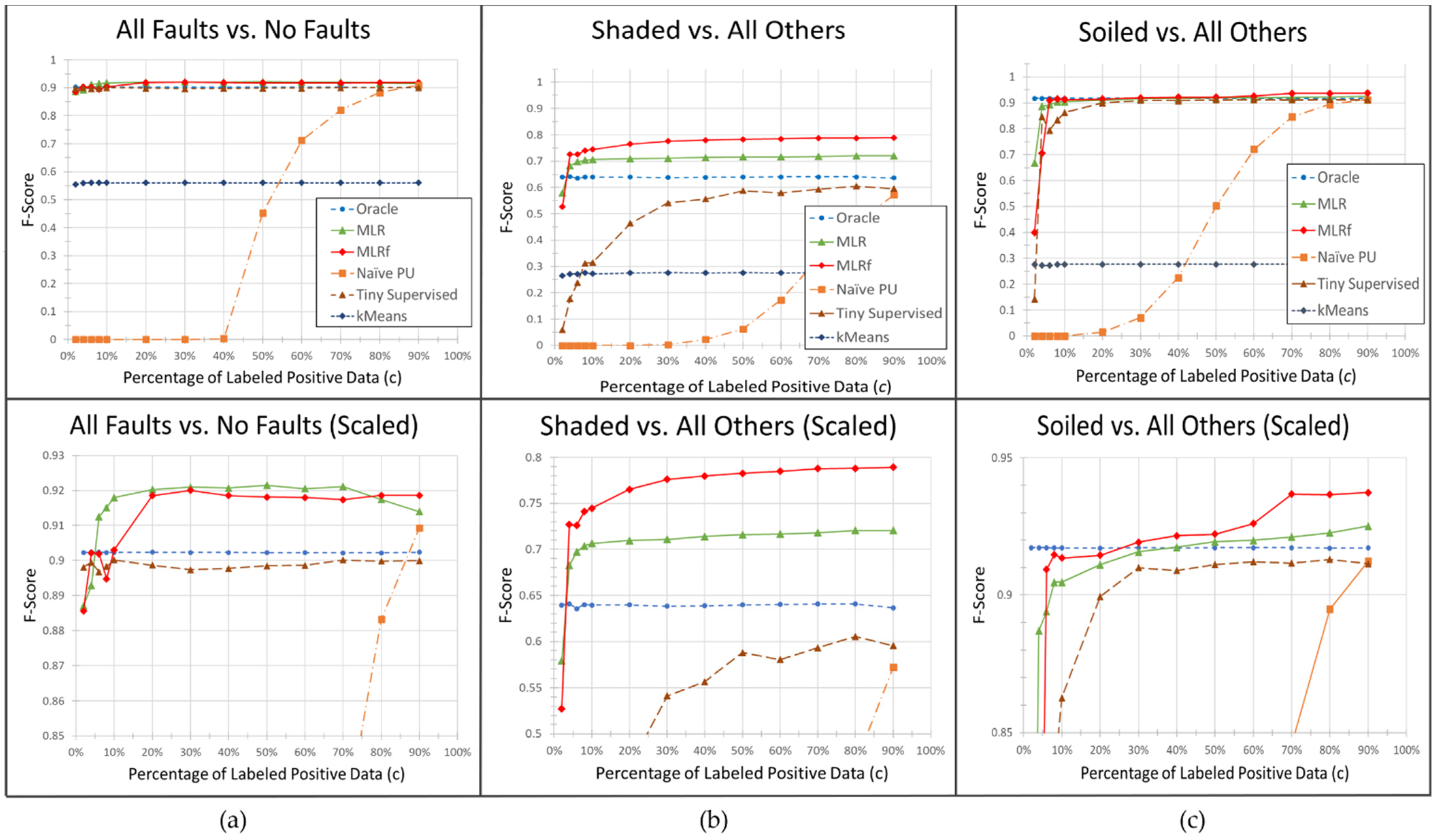
In the top graph in Figure 2a, we see that all algorithms including the MLR, MLRf, and “tiny” supervised learning algorithm behaved well and provided similar results, even with only 2% of total fault data labeled. As illustrated in Table 2, 344 datapoints out of 21,485 total datapoints were labeled at this lowest $c$ value. It should be noted that treating unlabeled samples as negatives, as illustrated by the naïve PU algorithm, is ineffective unless nearly all faulty points (17,188 total) are labeled. In the bottom graph, it is clear that both the MLR and MLRf algorithms slightly and consistently outperform the oracle and the “tiny” supervised learning algorithms when at least 10% of the positive samples are labeled. We believe this may be due in part to the non-linear classification capabilities of both algorithms. This is discussed further in the next bullet point.

• Shaded vs. All Others

Figure 2b demonstrates a situation where the nonlinear nature of the MLRf algorithm provides a clear advantage. The poor results of the supervised linear oracle model (with an F-Score of approximately 0.64) indicate that the faulty and non-faulty data for this problem are non-separable in the given feature space. The oracle model is underfitting the data. The improvement gained by the MLRf algorithm with its much higher feature dimensionality confirms this. If the decision boundary is substantially nonlinear, this could explain the noticeable F-score improvement of the non-linear MLRf classifier. A future test should be performed against a nonlinear oracle model for confirmation.

The more surprising result in this graph is the improvement made possible by the simpler MLR algorithm. The MLR algorithm has one additional variable over the oracle (the $b$ variable described in Section 2.2), and we surmise that this slight nonlinearity may be contributing to its success. It is remarkable that these high scores are possible even when only 4% of the faulty data is labeled, or 172 datapoints.

• Soiled vs. All Others

The soilage detection models in Figure 2c act similarly to those in Figure 2a in that the MLR, MLRf, and the “tiny” supervised algorithm are similar to that of the Oracle except at low values of $c$. Unlike the other graphs in Figure 2, MLRf performance increases noticeably above the Oracle only when the label frequency $c$ is around 70%—much higher than in other graphs. However, the actual difference is slight and may simply indicate an upward trend like that of the MLR algorithm. Due to the small number (five) of runs that we were able to do for this algorithm on this problem at that $c$ value, the jump at $c=0.7$ may be a random outlier. Additional simulations would need to be performed to test this hypothesis.

• Degraded vs. All Others

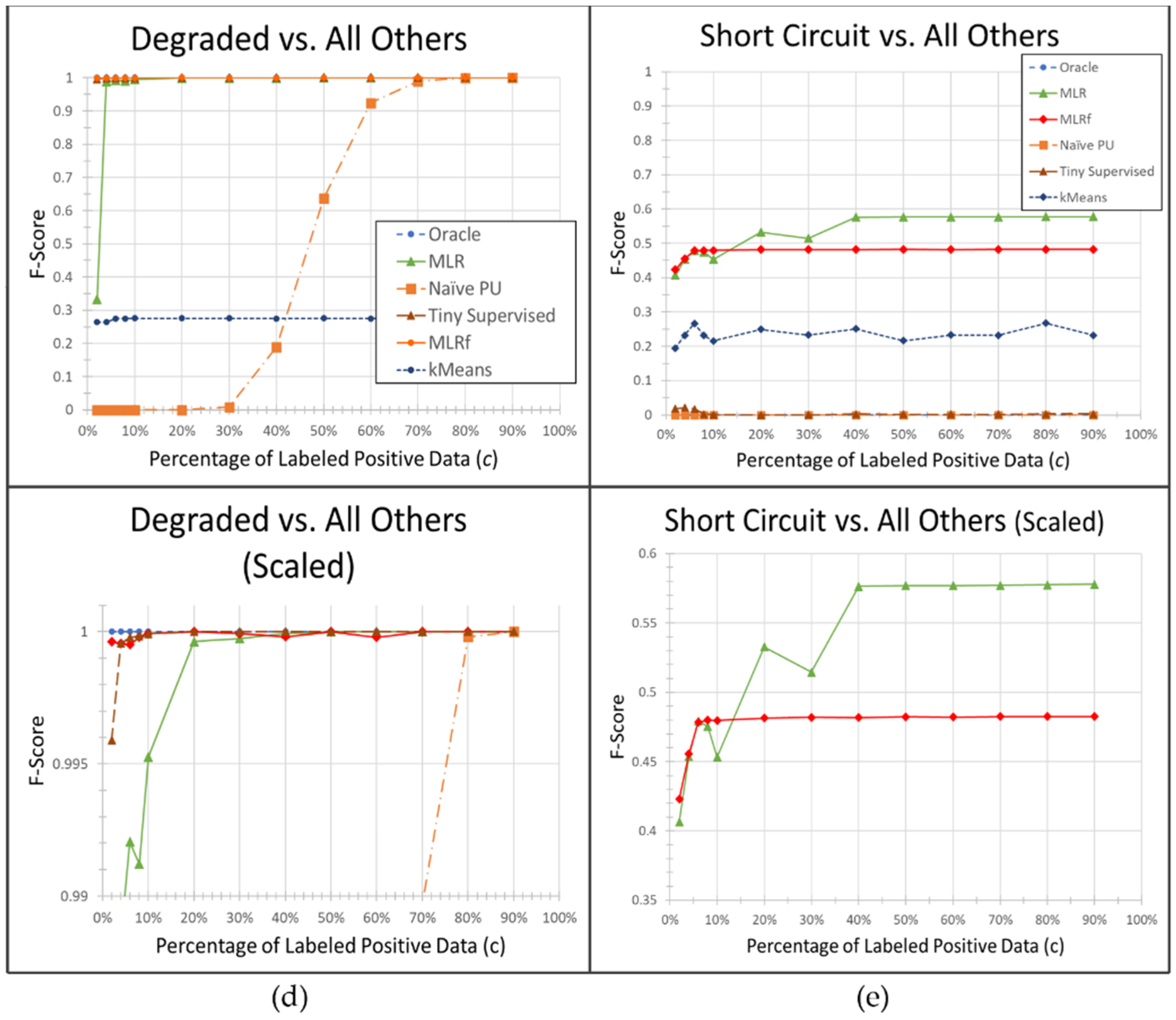
The degraded fault detection problem illustrated in Figure 2d is the “simplest” of all problems to solve in Figure 2. The oracle was able to achieve perfect classification (F-score = 1) in the given feature space for this problem. The MLR, MLRf, and “tiny” supervised algorithm also performed at or near this level for all but the very smallest of $c$ values. Notice that the lower graph had to be substantially scaled to see any variability between algorithms at all. Despite the obvious separability of this problem, neither the naïve PU algorithm nor the unsupervised k-means algorithm were useful.

• Short Circuit vs. All Others

Figure 2e illustrates our most interesting and enigmatic result. The oracle algorithm and related “tiny” supervised algorithm are unable to classify short circuit faults in the given feature space. The MLR and MLRf algorithms, while performing poorly with an F-score between 0.4 and 0.6, are nevertheless substantially more effective. Unlike the Shaded problem shown in Figure 2b, higher feature dimensionality alone is not sufficient to explain this discrepancy as the lower dimensional MLR algorithm performed better than the higher dimensional MLRf algorithm. One thought is that the MLRf algorithm with $p=3$ and $k=3$ expanded features may be overfitting the problem while the slight increase in dimensionality provided by the MLR algorithm may be preferable, though this conclusion is not particularly satisfying. Other authors such as [16] suggest that there are theoretical situations where PU learning can surpass supervised classification. It would be interesting to investigate if this is such a case. Either way, further research is warranted.

In addition to the increased dimensionality and non-linear models described above, one other possible improvement due to PU learning is possible. With noisy data, it may be that because of the reduction in labeled data in the positive class, outliers are likely to be excluded, simplifying the model, and improving overall performance. This does not seem likely to have played a large role in the given datasets however as the MLR and MLRf algorithm performance does not trend towards the oracle with higher values of $c.$ Instead, we believe that the non-linear aspects of the MLR and MLRf algorithms are more likely to explain this discrepancy as described in the bullets above. It is likely that this non-linear boundary can capture nuances that a fully linear boundary such as used in the simple supervised oracle algorithm used in this paper is unable to capture. feature engineering of the oracle algorithm or selection of a more advanced algorithm would likely improve this. Additionally, it may be worth investigating more theoretical explanations for these phenomena in future work as described in [16].

Due to the encouraging results, it is worth investigating these and other PU learning algorithms on additional solar fault datasets. The improvements in classification, with few labeled data samples, especially in the case of hazardous faults such as short circuits, bring significant value in terms of improved detection.

5. Conclusions

To the best of our knowledge, this is the first time PU learning has been used for solar fault detection and classification. This, along with the introduction of the MLRf algorithm in Section 2.3, comprise the novel contributions in this paper. PU learning has the advantage over standard supervised and semi-supervised learning in that it does not require any labeled data from the “good” or STC class. This allows seemingly faultless data to avoid additional expensive scrutiny to confirm faultless status. Mistaking a low-level fault for STC or treating unlabeled data as negative can confuse a learning algorithm and create a poor learning model, as shown by the poor results of the naïve PU algorithm in Figure 2 at lower values of $c$. At the same time, PU learning algorithms such as MLR and MLRf are extremely effective, essentially matching the quality of a fully supervised model at all but the very lowest possible percentage of labels. With a small amount of labeled fault data, PU learning can accurately label the large amount of unknown data as well as creating an effective model for future data. Comparisons with a “tiny” supervised learning algorithm in Figure 2a–c,e with the same number of labeled samples split between the positive and negative classes illustrate the benefit of PU learning and the advantage found in using the unlabeled data as stated in [17].

In addition to demonstrating the MLR algorithm on solar fault data, we proposed and evaluated a new MLRf algorithm developed for PU learning with application to solar fault datasets and other large datasets with few features. The MLRf algorithm has several components including feedback, feature enhancement, and feature pruning. These elements significantly increase the flexibility of the algorithm, though they do require additional hyperparameter tuning. They also raise the potential of overfitting concerns, though we did not see much evidence of this in our work.

Simulations were performed for PU labeled fault detection and classification for a variety of different $c$ values representing the percentage of known labels for the class of interest. Both the original MLR and the new MLRf algorithm provide extremely robust results, equaling or surpassing a fully supervised oracle algorithm when less than 10% of labels from the class of interest were available. These results are remarkable and confirm the results found in [13].