Advances in Simulating Radiative Transfer in Complex Environments

Abstract

Accurate simulation of radiative transfer is a very important aspect in climate modeling. For microclimate models in particular, it is not only important to simulate primary but also secondary radiative fluxes in great detail, i.e., emitted longwave and reflected shortwave radiation. As there are always limitations regarding computational effort and memory, these radiative fluxes are commonly implemented using simplified approaches. To overcome these simplifications and, thus, increase modeling accuracy, a new radiation scheme called indexed view sphere was introduced into the microclimate model ENVI-met. This new scheme actually accounts for radiative contributions of objects that are seen by each grid cell. In order to evaluate the advantages of the new scheme, it is compared against the formerly used averaged view factor scheme. The comparison in a complex realistic urban environment demonstrated that the indexed view sphere scheme improved the accuracy and plausibility of modeling radiative fluxes. It, however, yields an increased demand of memory to store the view facets for each cell. The higher accuracy in simulating secondary radiative fluxes should, however, overturn this shortcoming for most studies, as more detailed knowledge of local microclimatic conditions in general and eventually thermal comfort can be gained.

1. Introduction

Accurate modeling of radiative fluxes plays an important role in microclimatology. This is especially the case in urban areas, where large differences in radiative fluxes can be found due to complex structures, heterogeneous materials, and a multitude of different surface types [1,2,3,4,5]. While primary radiative transfer, i.e., incoming shortwave and longwave radiation, can be simulated quite easily using ray tracing algorithms and local sky view factors, simulating secondary radiative fluxes, which are emitted or reflected by objects of the environment (walls, roofs, the ground surface, or vegetation), are much more complicated to be modeled. The complexity in modeling these radiative fluxes lies in the multiple interactions between the different elements within the view range of the grid analyzed. For instance, radiation reflected by a surface will contribute to the incoming radiation received by other surfaces. These surfaces will again also re-reflect parts of this radiation and distribute in vicinity. Handling such complex conditions is a challenge that is common to all algorithms that involve simulating multiple reflections of radiation such as daylight simulation or image rendering in general [6,7,8,9,10].

Over the years, different approaches have been developed to tackle this problem using different kinds of numerical algorithms. The multiple reflections of shortwave radiation can, for example, be handled by tracing the reflected photons using a Monte Carlo approach [11,12,13,14,15]. For the analysis of more mono-directed rays originating from discrete light or radiation sources, raytracing algorithms can be used to follow the radiation on its path through the modeled environment, similar to the algorithms implemented in the microclimate model ENVI-met to calculate the shadow casting [16,17,18,19]. Another group of algorithms approaches the problem from the other side, by not tracing the radiation itself, but analyzing the view relations between the different emitting and receiving elements in a scene or environment. These types of algorithms are generally categorized as radiosity approaches, with several sub-groups depending on the way the individual interactions between the elements are solved (e.g., matrix radiosity, progressive radiosity, or wavelet radiosity) [20,21,22,23,24,25,26,27].

While these methods give good results in smaller environments such as indoor spaces, they are hardly applicable for outdoor situations where an enormous number of elements and view relations between points in space need to be analyzed due to the larger and more complex geometries. Moreover, different to indoor environments, where the radiative fluxes are often calculated only once for a given setting, the situation in an outdoor environment is constantly changing due to movement of the sun and the resulting heating and cooling of surfaces. Hence, the radiative situation needs to be solved frequently—similar to the shadow casting, which is typically updated every few minutes [28].

Modern microclimate models such as the CFD-model ENVI-met that considers turbulence and is based on solving Reynolds–Navier–Stokes equations [28,29,30,31], allow for a very precise representation of the urban environment: Besides the detailed plant model [32,33], ENVI-met recently introduced an Accurate In-Canopy Radiation Transfer scheme, which accounts for scattering and attenuation of shortwave radiation within trees’ canopies [34]. Buildings cannot only be digitized with a variety of different materials but also individual façades of the same building can consist of different materials [28,35,35,36]. The same is possible with the ground surface, where different surface types can be assigned to every grid. Since the different objects, materials, and surface types carry their own physical parameters such as albedo, emissivity, heat transfer coefficient, etc., the possibility to accurately replicate the variety of the urban environment drastically increases the accuracy of the model results. In previous versions of ENVI-met, however, the effects of different materials and surfaces were only calculated explicitly for primary radiation [37]. The distribution of secondary radiative fluxes (reflected shortwave radiation and longwave radiation emitted from objects) was, due to lack of memory and to save computational effort, carried out using a simplification, where instead of the actual reflected shortwave radiation and longwave radiation emitted, averages over all façades and surfaces within the model area were used [37]. This simplification could in some instances lead to a rather low accuracy that has been reported in evaluation studies comparing modeled against measured values of radiation and mean radiant temperature (MRT) [30,38,39,40,41,42,43,44].

In this paper, a newly developed method is introduced to overcome these shortcomings. It enables the simulation of fluxes of reflected shortwave and emitted longwave radiation within the urban environment with a much higher level of detail, considering the actual objects, i.e., façades, surfaces, and trees “seen” by a grid cell. By simulating secondary radiation in greater detail, differences in local microclimates can be identified more clearly and influences of, e.g., highly reflective surfaces or vegetation cover onto bioclimate indices such as physiological equivalent temperature (PET) can be taken into account. In a large ENVI-met proof-of-concept simulation featuring a multitude of different surfaces and plants, the new method is compared against the previous approach. The comparison should evaluate the accuracy of the new radiation scheme and examine the impacts of the more accurate secondary radiation modeling on the simulated local microclimate.

2. Model Description

In the following, the old averaged view factor concept used in ENVI-met is described (Section 2.1) and the advancements of the new indexed view sphere (IVS) algorithm are laid out in detail (Section 2.2). To evaluate the advantages of the new IVS module, a proof-of-concept simulation is conducted comparing the results of both concepts (Section 2.3).

2.1. The Averaged View Factor (AVF) Concept

To describe the radiative situation and solve the interactions between different elements, ENVI-met version 4.4.5 and prior used a generalized visibility concept based on averaged view factors (AVF). In the AVF concept, first, a three-dimensional ray tracing analysis is performed for every cell. Starting from a grid cell’s center, rays are being shot for every 10° height and 10° azimuth angle creating a sphere consisting out of 18 × 36, thus 648 individual view facets. While calculating these 648 individual view facets for every grid cell can be very time consuming, it only needs to be performed once for a model simulation as the objects seen by a cell do not change over the course of a simulation. Based on the object type (sky, building, plant, ground surface) seen by the view facet/hit by the ray and the total number of view facets, averaged view factors of sky ${\sigma }_{Sky}$, vegetation ${\sigma }_{Veg}$, buildings ${\sigma }_{Bldg}$, and ground surfaces ${\sigma }_{Grnd}$ were stored as single values for each grid cell. By only saving the view factors for the different object types instead of the actual façade elements, ground surfaces, and plant sections seen in the facets, a lot of memory can be saved. However, since no information is stored about which individual elements are in radiative exchange with the cell, the calculation of secondary radiative fluxes cannot take into account the radiation exchanges between actual objects seen but rather has to resort to an approximation. Instead of individual information about radiation received from particular objects, the secondary radiation is approximated by combining a grid cells’ view factor for buildings, plants, and ground surfaces with averaged values of reflected and emitted longwave radiation for all buildings, plants, and ground surfaces over the entire model domain [19,28,37].

The received secondary radiation of a cell—in this case, the received shortwave reflected radiation from buildings—is, thus, calculated by:

$$Q_{swrefl,in}\left(i,j,k\right)={\sigma }_{Bldg}\left(i,j,k\right)·Q_{Bldg,swrefl}$$

(1)

with ${\sigma }_{Bldg}\left(x,y,z\right)$ as the building view factor (0 to 1) of cell $i,j,k$ and $Q_{Bldg,swrefl}$ as the averaged reflected shortwave radiation from all buildings calculated by:

$$Q_{Bldg,swrefl}=\frac{1}{N}{\displaystyle \sum }_{a=1}^N\propto \left(a\right)·Q_{sw}\left(a\right)$$

(2)

with $N$ being the total number of façades in the model, $\propto$ the albedo of façade $a$, and $Q_{sw}$ the shortwave radiation in front of façade $a$. The same calculations are carried out taking into account averaged surface temperature values of buildings, leaves, or ground surfaces for the estimation of received secondary longwave radiation.

To account for changes in the radiative situation, these calculations (Equations (1) and (2)) and their respective counterparts for other object types and emitted longwave radiation need to be solved regularly, i.e., every 15 min by default in ENVI-met.

The consequence of this simplification is that every point with an identical view factor for buildings, ground surfaces, or vegetation will receive the exact same amount of reflected shortwave and emitted longwave radiation.

While this simplification does save memory, it also leads to very unrealistic results: Given the same view factors, a cell would receive the exact same amount of reflected shortwave and emitted longwave radiation independent of the actual radiative processes in its vicinity. This could lead to identical reflected shortwave fluxes in front of north and south façades or high-reflective façade materials or low-reflective façade materials.

2.2. The Indexed View Sphere (IVS) Algorithm

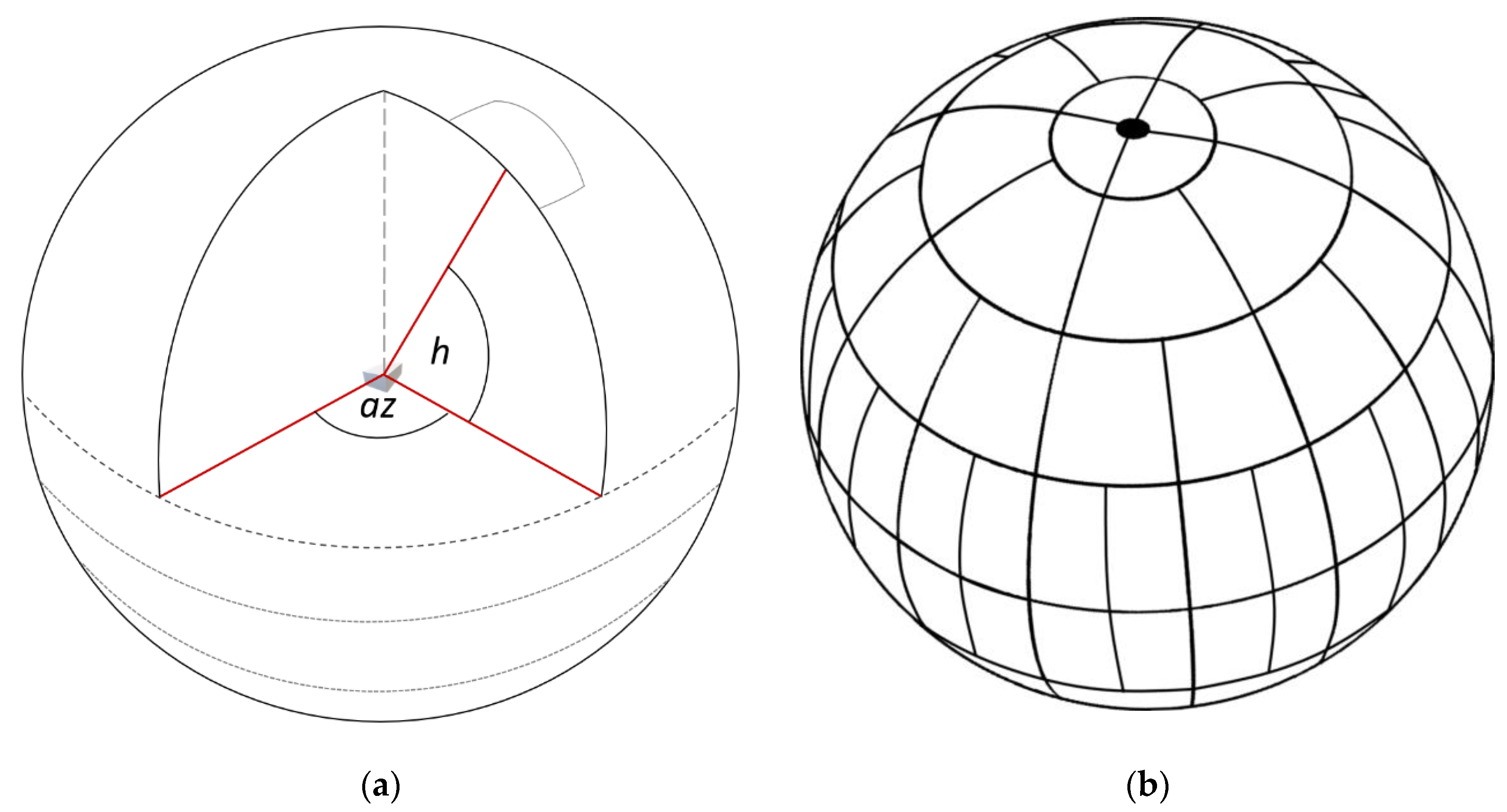
To overcome this simplification, the indexed view sphere (IVS) algorithm was developed and implemented into ENVI-met. The main idea behind IVS is to save the results (i.e., the objects seen by a cell in a certain view angle) of the initial geometrical analysis so that it is possible to relate the calculated view factors back to the contributing elements of the urban scene. Its fundamentals are comparable to sky view factor calculations based on fish-eye imagery where the amount of sky pixels per annulus ring is analyzed (Figure 1a) [45,46,47,48]. To reduce the memory needed, the new IVS does not calculate the same amount of view facets in all height angles of the view sphere (Figure 1b).

Since the resulting surface area for a given azimuthal angle decreases with increased height angles, the size of the azimuthal angle and, thus, of the view facets can be set larger with little to no information loss. The size of the azimuthal angles and, thus, the view facets is calculated by a function of the height angle. The user only defines the resolution of the height angles and the azimuthal angles at the equator of the cell. The number of azimuthal angles, i.e., the number of distinct view facets for a given height angle is then calculated by:

$$\lambda \left(h\right)=\frac{360}{a{z}_{eq}}·\cos \left(h\right)$$

(3)

with $a{z}_{eq}$ as the user defined size of azimuthal angle at the sphere’s equator and the height angle $h$. To ensure all cardinal directions are represented, a minimum of four azimuthal angles is set for height angles less than |90°|. For height angles of ±90° only one view facet is obtained, since azimuthal angles would be indifferent for these height angles.

By reducing the number of view facets per cell, an immense amount of memory can be saved without losing too much information about objects seen by a grid cell. Where a 10° height and azimuthal angle would previously result in 648 view facets, the same height and azimuthal resolution at the equator now results in 414 view facets. In combination with more efficient data structures, this decreases memory demand by around 40% and enables the possibility to store pointers to the objects seen by cells in a particular direction. By storing a direct link to objects seen by a cell, the actual radiation reflected/emitted by these objects can now be used to calculate a cell’s received reflected shortwave and longwave radiation instead of using averaged values. Taking into account this radiation received, the cell alters its own reflection of shortwave and emission of longwave radiation and in turn contributes to the radiation received of other cells.

To calculate the received reflected shortwave and emission of longwave radiation coming from buildings or ground surfaces, the individual contribution of the objects is weighted by the view angle of the facet and simply added up:

$$Q_{Build,Grnd,in}\left(i,j,k\right)={\displaystyle \sum }_{a=1}^F\omega \left(a\right)·{\tau }_{Veg}\left(a\right)·Q_{Build,Grnd,out}$$

(4)

with $F$ being the total number of facets of the view sphere, $\omega \left(a\right)$ as the weight of the view facet $a$, ${\tau }_{Veg}\left(a\right)$ as the transmission factor accounting for reduction of the visibility due to vegetation between the cell $i,j,k$ and the objects seen, and $Q_{Build,Grnd,out}$ as the outgoing reflected shortwave or emitted longwave radiation by the seen objects.

Secondary radiation emitted by vegetation is accounted for by inverting the transmission factor:

$$Q_{Veg,in}\left(i,j,k\right)={\displaystyle \sum }_{a=1}^F\omega \left(a\right)·\left(1-{\tau }_{Veg}\left(a\right)\right)·Q_{Veg,out}$$

(5)

with $Q_{Veg,out}$ as the outgoing reflected shortwave or emitted longwave radiation by the seen plants.

While the height angles are constant within a view sphere, the azimuthal angle and, thus, the number of view facets changes with increased height angles. This implies that the weighing factor is not identical for all view facets, but depended on the number of view facets in a particular height ring. The individual weighting factor accounting for the contribution of a view facet is calculated by:

$$\omega =\frac{1}{\lambda \left(h\right)}·\frac{1}{r_{cnt}}$$

(6)

with $\lambda \left(h\right)$ as the number of view facets in a given height angle and $r_{cnt}$ as the number of height rings for a particular view direction, e.g., downward view or upward view.

The transmission factor for vegetation ${\tau }_{Veg}$ is calculated within the raytracing and accounts for a partial obstruction of radiation due to vegetation in the ray’s path. The calculation of transmission is carried out using the exponential extinction coefficient accounting for leaf orientation $\phi$ (currently set to 0.5), the local leaf area density (LAD), and the path length through the vegetation cells:

$${\tau }_{Veg}={ \mathrm{e}}^{-\left(\phi · \mathrm{LAD}·dRay\right)}$$

(7)

Further advancements have been undertaken with regards to the ray tracing algorithm. While in previous versions, the segment length for the ray would be determined only once for a given angle, the new algorithm tries to find an appropriate length for the ray segments based on current grid dimensions as well as the azimuthal and height angle. Determining a segment’s length is not only critical for the calculation speed as short rays drastically increase computational effort but also for the quality of the resulting radiation calculation. With the discretization of space in models such as ENVI-met an optimal ray length is very hard to determine. With typical cell dimensions of 2 to 5 m in x, y, and z [28], too short ray segments might lead to an over-representation of cells, which are only marginally clipped by a ray, since the whole cell would count as “hit” by the ray. Too large ray segments, however, might lead to not detecting/not taking into account objects in the path of a ray.

To determine an optimal vector length increment for the ray trace, given the azimuthal and height angle, the normalized contribution weight ($d{x}_{nwght}$, $d{y}_{nwght}$, and $d{z}_{nwght}$) of the x, y, and z axis onto the resulting vector is calculated at first:

$$\begin{gathered} \left(\begin{array}{c}d{x}_{wght}\\ d{y}_{wght}\\ d{z}_{wght}\end{array}\right)=\left(\begin{array}{c}|\cos \left(h\right)·\cos \left(az\right)|\\ |\cos \left(h\right)·\sin \left(az\right)|\\ \left|\sin \left(h\right)\right| \end{array}\right) \\ dxy{z}_{Sum}=d{x}_{wght}+d{y}_{wght}+d{z}_{wght} \\ \left(\begin{array}{c}d{x}_{nwght}\\ d{y}_{nwght}\\ d{z}_{nwght}\end{array}\right)=\left(\begin{array}{c}d{x}_{wght}/dxy{z}_{Sum}\\ d{y}_{wght}/dxy{z}_{Sum}\\ d{z}_{wght}/dxy{z}_{Sum}\end{array}\right) \end{gathered}$$

(8)

By taking into account the cell dimensions of the current cell, the normalized weights for all axes are then used to scale the length of the three-dimensional vector:

$$dRay\left(i,j,k\right)=\vartheta ·\left(dx\left(i,j,k\right)·d{x}_{nwght}+dy\left(i,j,k\right)·d{y}_{nwght}+dz\left(i,j,k\right)·d{z}_{nwght}\right)$$

(9)

with $\vartheta$ as a scaling factor of the vector length. This scaling factor should ensure that cells are detected, which only partially lie along the path of the vector, i.e., a segment of the ray ends within the cell’s boundaries. While a small scaling factor ensures a very precise ray tracing detecting all cells hit by a ray, it also leads to increased calculation time. Even more importantly, cells that might only lie very marginally in the path of the ray, i.e., clipped only very slightly, may be overrepresented in the further calculation. Test simulations showed that a scaling factors between 0.25 and 0.5 led to a good compromise between accuracy of the ray tracing and representation of cells clipped by the ray.

To determine the increments in the x, y, and z direction, the calculated vector length $dRay\left(i,j,k\right)$ is then again calculated by:

$$\left(\begin{array}{c}d{x}_{seg}\\ d{y}_{seg}\\ d{z}_{seg}\end{array}\right)=\left(\begin{array}{c}dRay\left(i,j,k\right)·\cos \left(h\right) ·\cos \left(az\right)\\ dRay\left(i,j,k\right)·\cos \left(h\right) ·\sin \left(az\right)\\ dRay\left(i,j,k\right)·\sin \left(h\right) \end{array}\right)$$

(10)

After each iteration, the ray length for the current grid cell is updated to account for non-equidistant gridding in the model.

The new IVS calculation method for calculating secondary radiation transfers can be enabled in the simulation settings of the SIMX file. By default, the module is switched off. If enabled, the user is able to adjust the height angles and azimuthal angles at the sphere’s equator. To save memory, the simulation settings allow us to define a high-resolution and a low-resolution angle pair. After a cut-off height defined, the model switches from the sphere definition of the high-resolution angles to the low-resolution angles. Similar to ENVI-met’s vertical splitting (see [28]), radiation processes near the surface can, thus, be modeled with higher accuracy while processes of secondary radiation transfer above are carried out in a coarser resolution. This not only saves memory but also computational power. In case the user does not want to use this option, the high-resolution and low-resolution angles can simply be entered identically.

2.3. Proof-of-Concept Simulation

The advancements of ENVI-met’s new IVS module are evaluated by comparing the model results of a simulation featuring the old AVF concept against a simulation featuring the new IVS algorithm, respectively. The model results will first be compared against each other with regard to longwave and shortwave radiation patterns, MRT, and potential air temperatures for different heights and times during the day. Furthermore, the impact of simulating secondary radiative transfers using IVS is examined by comparing the thermal comfort index PET between the two simulations.

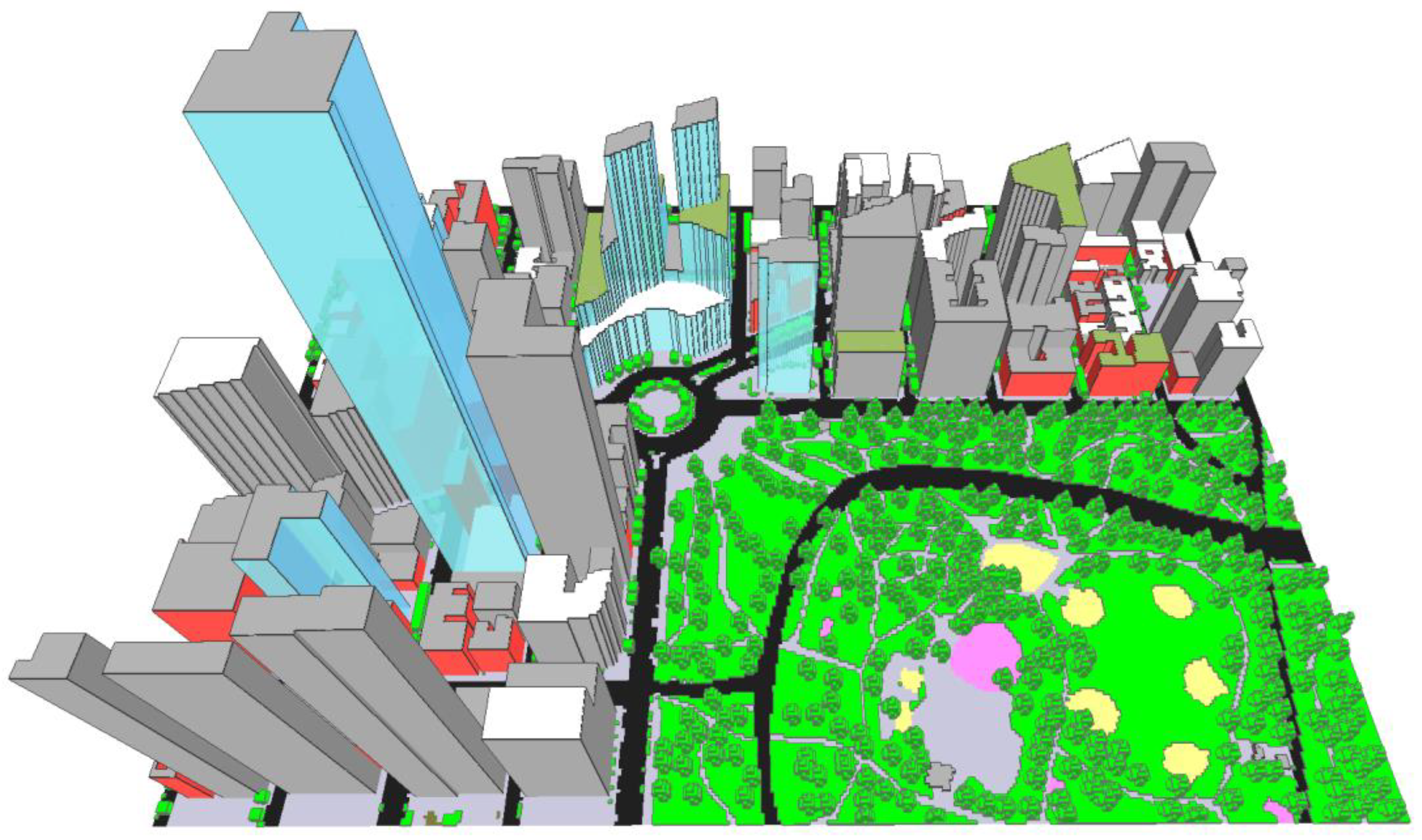
In order to find the expected large differences in radiation budgets—and, thus, in the resulting microclimate conditions—between varying surface and building materials, the modeled area was chosen based on high spatial variability. The model area is located at the edge of Central Park in New York City, NY, USA featuring an additional high recognition value because of its iconic urban morphology surrounding the Columbus Circle. Varying building heights, differing materials such as glass, concrete, or brick and specific roof types such as roofs featuring greenery or cool (high-albedo) materials, which are common heat mitigation measures [49,50], already show the heterogeneity of the model area. Furthermore, the great differences in surface materials (meadows, rocks, sand pitches, streets, and pavements) together with the dense tree vegetation in Central Park located in a model area’s lower right will enable us to show the complexity in secondary radiative fluxes that can be modeled by the new IVS module. To show the large variety of building and surface materials, the different materials have been visualized by specific colors (Figure 2).

Table 1. Summary of material properties in the proof-of-concept simulation [51].

	Layer	Name	Albedo	Absorptivity	Emissivity	Thickness [m]	Conductivity [W (m K)−1]	Density [kg m−3]	Specific Heat (J (kg K)−1)
Concrete Wall	Outside	Concrete	0.2	0.8	0.9	0.2	1.311	2240	836.8
	Middle	Steel frame Insulation	0.2	0.8	0.9	0.08	0.049	265	837
	Inside	1/2IN Gypsum	0.2	0.8	0.9	0.01	0.16	785	830
Glass Wall	All	Glass	0.25	0.05	0.94	3 × 0.01	0.029	830	840
Brick Wall	All	Brick	0.15	0.85	0.9	3 × 0.08	0.66	1500	1000
Default Roof	Outside	Default membrane	0.2	0.8	0.9	0.01	0.16	1121	1460
	Middle	Insulation	0.2	0.8	0.9	0.14	0.049	265	837
	Inside	Metal Decking	0.2	0.8	0.9	0.01	45	7680	418
Cool Roof	Outside	Cool material	0.65	0.35	0.9	0.02	0.85	1200	1200
	Middle	Insulation	0.2	0.8	0.9	0.14	0.049	265	837
	Inside	Metal Decking	0.2	0.8	0.9	0.01	45	7680	418

gives an overview on the parameters of these materials that are based on the Midrise Apartment Post 1980 Standard for American Housing in NYC [51]. Building footprints and street tree locations were retrieved from the NYC open data portal [52]. Surface and building materials as well as park trees were digitized based on aerial imagery.

The meteorological boundary conditions were taken from an Energy Plus Weather File of NYC [53]. To resemble a hot summer day with clear sky conditions, July 21st was selected as simulation date. The simulation has been run for 24 h. Figure 3 shows the meteorological conditions for the whole simulation period provided by the EPW-file.

General simulation and model area properties are described in

Table 2. Parameters of the proof-of-concept simulations.

General Properties of Both Simulations
Start Date and Time (Local)	21.07.2017 05:00
Duration [h]	24
Wind Speed [m s−1]	2
Wind Direction [°]	325
Meteorological Boundary Conditions	Full Forcing
Location Lat (Lower Left Corner)	40.76° N
Location Lon (Lower Left Corner)	−73.98° E
Dimensions	360 × 260 × 52
Resolutions (X, Y, Z) [m]	2.5 × 2.5 × 5
Lowest Grid Cell Split	Yes
Telescoping: Factor and Starting Height	30% above 180 m
Height of 3D Model Domain [m]	1434 m
Building Indoor Temperature Held Constant at	20 °C
View Factor Update Interval	30 days
Specific Radiation Scheme Settings for IVS Simulation
Height Angle High Resolution Near Ground	15°
Azimuthal Angle High Resolution Near Ground	15°
Height Angle Low Resolution Above Height Boundary	30°
Azimuthal Angle Low Above Height Boundary	30°
Height Boundary between High and Low Resolution	8 m

. Air temperature within buildings is held constant at 20 °C to account for the strong air conditioning cooling used in almost every building in NYC. Radiation scheme settings for the IVS simulations feature medium resolutions for lower cells at pedestrian level and low resolutions for higher cells above 8 m. Due to the large size of the model area featuring high-rise buildings and covering multiple different urban morphologies and typologies in a high spatial resolution, IVS settings could not feature higher view facet resolutions due to memory limitations. With these settings, the simulation yields around 50 GB of RAM for the IVS simulation.

3. Results and Discussion

To give an overview on the differences between AVF and IVS, visualizations of the case study simulation results are presented. Radiation patterns as well as temperature distributions and impacts on thermal comfort are compared using absolute value maps of both scenarios to evaluate the advancements provided by the new IVS scheme.

After the theoretical explanations in Section 2.2., principles in IVS modeling are visually demonstrated by the 3D view of the model area. Figure 4 shows the rays that were traced for one specific grid cell at 138, 150, 6 amid the center of Columbus Circle. Each ray represents a view sphere segment of the grid cell to be analyzed. It is emitted from the grid cell center and searches for objects in each view sphere direction. When a building or soil surface is hit, the raytracing is aborted, and the object information is stored. With increasing height angle and especially above the highest object height, the length of each raytracing segment is, to save computational time, drastically increased as the probability of hitting an object is diminishing.

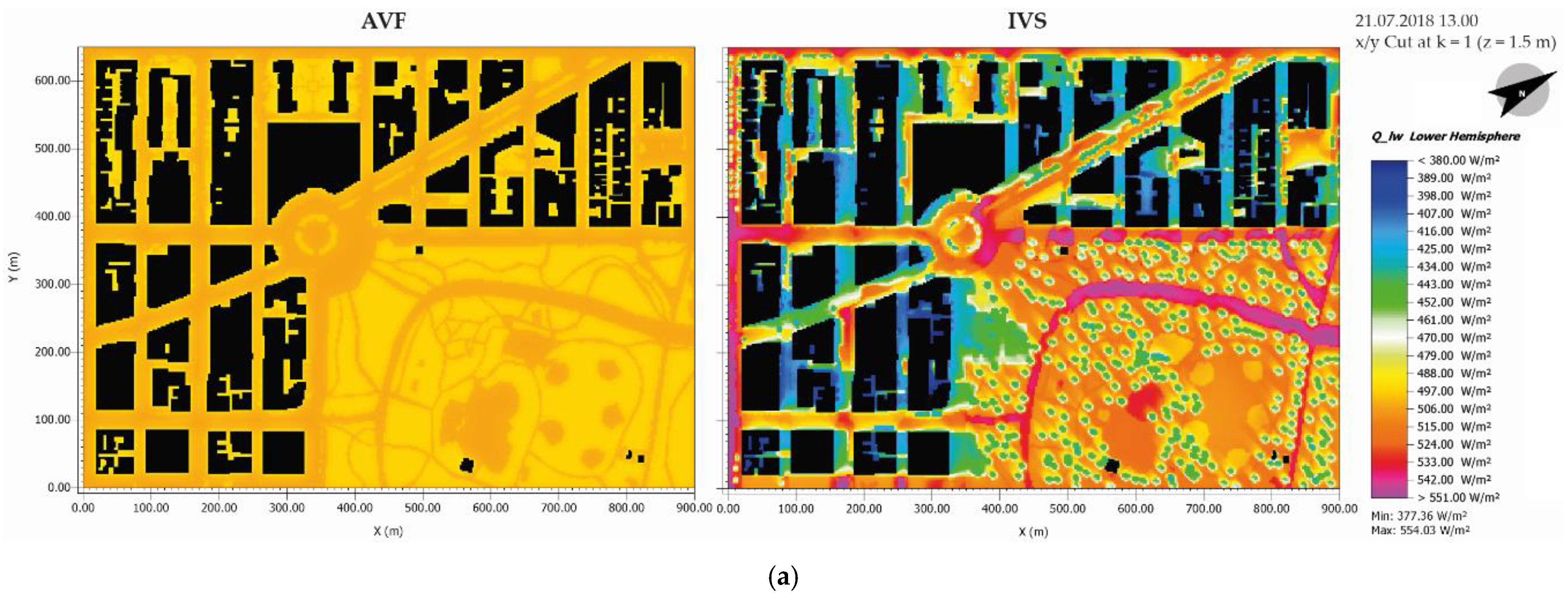
ENVI-met provides multiple output variables to allow the analysis of radiation patterns. Variables containing shortwave or longwave radiation values are distinguished between the upper and lower hemispheres to allow for a specification from which direction the radiation is received. Analyzing, for example, longwave radiation distribution received from the lower hemisphere in a horizontal cut at 1.5 m height, most radiation input probably originates from soil surfaces, ground vegetation, and nearby façade elements. Figure 5a demonstrates that longwave radiation values cover a wider range and more distinct differences over the model at 13:00 in the IVS scenario compared against the AVF scenario. Especially the pattern of park streets can be recognized, as they emit more longwave radiation than their surroundings. That is caused by their low-albedo surfaces that heated up more during the morning hours in contrast to the street canyons, which have been shaded by buildings. In IVS, dotted patterns of lower longwave radiation values received by the lower hemisphere can be found in Central Park where trees cast shade and, thus, cool the ground below canopies leading to less longwave emission compared to the open surfaces in other park areas. These patterns are still visible in Figure 5b depicting the same results but for a horizontal cut in 82.5 m height. Furthermore, as the cut is performed in an intermediate height—above some low- and medium-rise buildings of the model area—differences in roof type effects can be examined. In IVS, the rather cold—and thereby not emitting much longwave radiation—cool and green roofs stand out against the traditional hotter low-albedo roofs that strongly contribute to the longwave radiation received in 82.5 m height. In AVF with its averaging approach, these different roof surface temperature differences while being simulated to not translate in differences of emitted longwave radiation as their contribution as specific object is not stored individually. Even differences in longwave radiation values caused by trees in Central Park are still recognized by IVS, even though spatial distances between the grid cells in 82.5 m height and the trees at ground level are quite large.

While surface temperature mainly drives the emitted longwave radiation patterns, reflected shortwave radiation is influenced by both albedo and shadowing. Figure 6a clearly demonstrates which areas are shaded during 13:00 when the sun’s position is in the South—thus being at the model area’s left due to its rotation. Figure 6a,b again show less pronounced differences in AVF. Especially the very small range between 90 and 144 W/m² at pedestrian level in AVF shows that most parts of the model area are rather homogenously affected by reflected shortwave radiation. The IVS results, however, accurately account for spatial relationships between objects and, thus, the models minimal reflected shortwave radiation of <5 W/m² for shaded areas but very large contributions of reflected radiation in high-albedo spots, for example above open sand at the ballpark in Central Park.

Furthermore, when performing a horizontal cut at 82.5 m height, we again find roofs in IVS to show higher values than other parts of the model area in contrast to AVF. However, their higher albedo, green and especially cool roofs now show higher values, as they reflect more shortwave radiation than the traditional low-albedo roofs. By examining these comparisons in Figure 5 and Figure 6, it becomes clear that both longwave and shortwave contributions to a cell’s radiation budget are underestimated by AVF. Urban heating caused by traditional building materials as well as cooling performances of cool or green roof application, hence, probably have been underestimated in previous ENVI-met modeling studies [30].

By using the model area average, AVF does not consider shortwave radiation reflections accurately in general, which is proved by two additional examples. It is firstly shown by the comparison of reflected shortwave radiation patterns for the horizontal cut at 82.5 m at 09:00 where the sun’s position is in the east coming from the bottom side of the model area (Figure 7a). Since the circular shaped building at the Columbus Circle features glass façades and, thus, works like a magnifying glass, shortwave radiation is reflected from all sides to the center, which leads to a high accumulation in sum. By using IVS, these reflections are accounted for and values of up to 299 W/m² amid the circular-shaped building wall at the Columbus Circle are predicted by the model, whereas AVF only shows very low values around 25 W/m² here.

Secondly, the pedestrian level horizontal cut of shortwave radiation reflections from the upper hemisphere also shows that, in contrast to AVF, IVS takes the reflection of glass façades into account (Figure 7b). As solar radiation at 13:00 originates from the south being at the left-hand side of the model area, shortwave reflected radiation coming from upper wall parts is modeled to be received in urban canyons at pedestrian level on the left-hand side of glass-façade buildings. The total amount, however, is comparatively low, as solar radiation is mostly reflected upwards from soil or roof surfaces and is, thus, included in the lower hemisphere values. Besides the primary reflection from wall surfaces, secondary reflected radiation can be found in Central Park, where primary reflected solar radiation from soil surfaces and grass is secondarily reflected downwards by tree canopies.

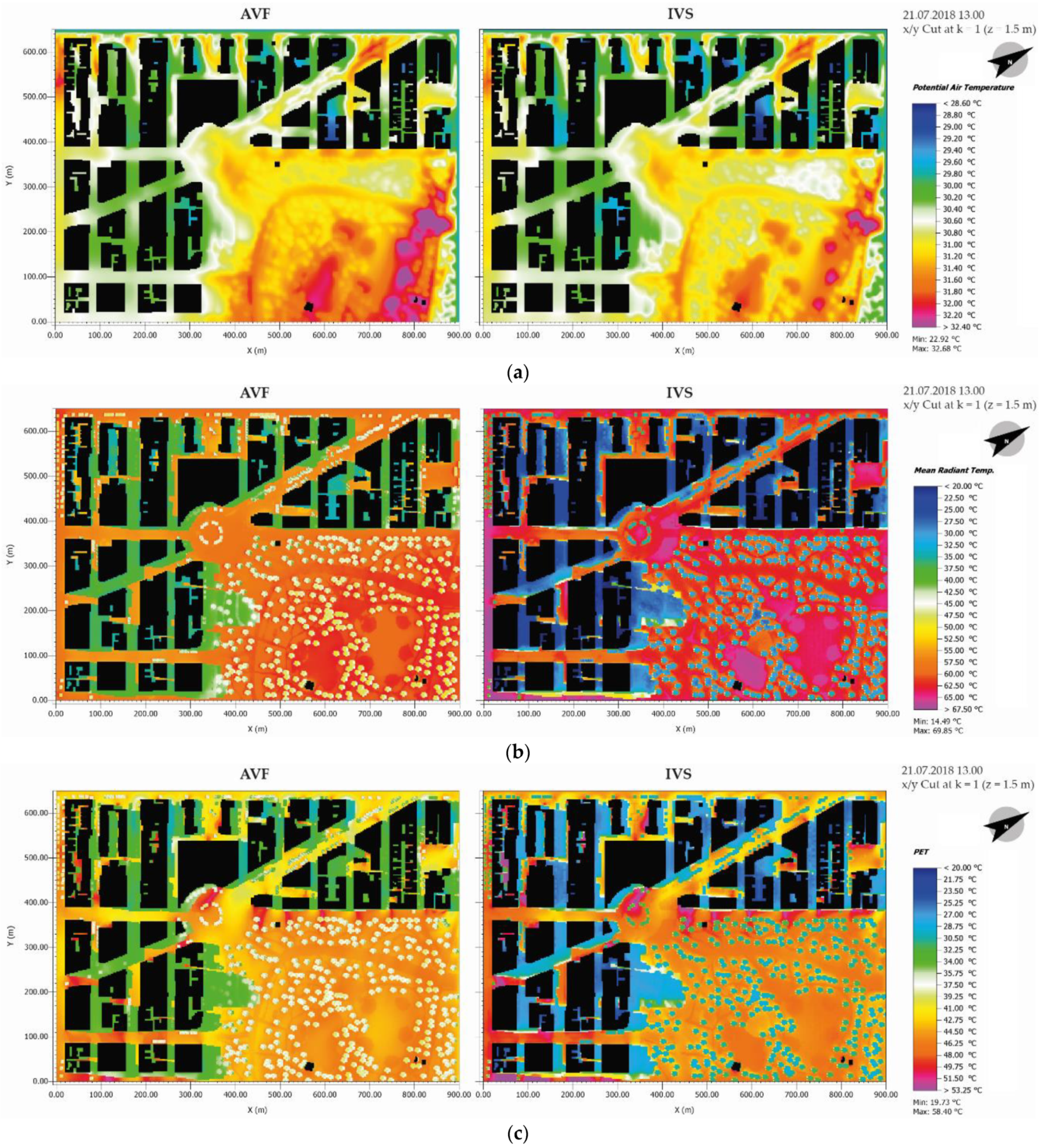
In contrast to the massively differing radiation patterns, at first glance, we only find small discrepancies in potential air temperature results for a horizontal cut at pedestrian level at 13:00 between AVF and IVS (Figure 8a). In general, IVS features slightly lower values of around 0.2–0.4 K. However, we find distinct differences between AVF and IVS in parts where high discrepancies of secondary radiation fluxes were observed. Especially the cooler regions in the southern/left part of the model area are more pronounced in IVS, as they receive less emitted longwave and less reflected shortwave radiation due to the shadows of larger skyscrapers next to them.

Analysis of MRT corroborates that by showing even larger deviations between AVF and IVS for the same height and timestep (Figure 8b). According to the radiation patterns the MRT is based on, MRT also features a wider range of values in IVS.

To address the magnitude of urban heat stress and the effects of mitigation strategies properly, thermal comforts indices are often used as holistic indicators in urban environments. These indices take several parameters such as air temperature, humidity, wind speed, and MRT into account [54,55]. In this study, the thermal comfort index PET is used representing a commonly used index for outdoor environments of temperate climate zones [56,57,58]. When analyzing PET in Figure 8c, we find that major patterns are the same between AVF and IVS. However, the range is again wider and more differentiated in IVS simulation. As discrepancies in wind field and humidity are assumed to be marginal by the use of different radiation schemes and as temperatures are shown to be only slightly different in Figure 8a, deviations are mainly based on the differences in MRT patterns, which are in turn a key factor for thermal comfort and, thus, PET calculation.

These findings agree with the analysis of nighttime results shown in Figure 9. Longwave radiation emissions are based on the object temperatures. During nighttime, these surface temperatures of soils, buildings, and plants are influenced by their thermal properties, which specify their behavior in storing and releasing heat, as well as the amount of solar radiation that has or has not been received during daytime. As both of these parameters vary massively over the model area, simulated surface temperatures and, hence, longwave radiation patterns should differ as such. However, only in IVS, these very fine and distinct patterns of emitted longwave radiation from the lower hemisphere are recognized for both urban canyons as well as Central Park in the horizontal cut in 1.5 m height at 03:00 (Figure 9a). AVF, in contrast, shows a uniform distribution of values around 415 W/m² for all parts of the model area. As thermal comfort indices take MRT into account and MRT is solely based on longwave radiation during nighttime, the high accuracy in modeling longwave radiation budgets, when using IVS compared to AVF, improves the accuracy and reliability of thermal comfort indices. High accuracy for modeling nighttime urban heat stress is especially needed for metropolitan regions where thermal stress at nighttime can lead to health implications such as insomnia or cardio-vascular diseases [59]. In the comparison of PET results at pedestrian level for 03:00 (Figure 9b), we indeed find some discrepancies in defining thermal hotspots between both scenarios. By including more precise MRT values into thermal comfort calculations, PET is refined and mostly decreased in almost all parts of the model area. Cooling influences of Central Park for the built-up areas, however, cannot be observed as the wind flows in from the top of the model area and leaves at the open park side at the bottom of the model area. Since the influence of both shortwave and longwave radiation patterns on thermal comfort proves to be very large, the new IVS scheme seems to be able to contribute to a more accurate analysis of urban thermal comfort in general.

4. Conclusions

In order to improve microclimatological analysis of complex urban environments, a new radiation scheme is introduced into the microclimate model ENVI-met. In contrast to the old AVF scheme, where view factors are averaged over the whole model area, the new IVS scheme is able to analyze the surrounding objects of each grid cell and calculate their contribution to the local radiation budget. The high accuracy of modeling secondary radiative fluxes such as emitted longwave radiation and reflected shortwave radiation by using IVS was demonstrated by a proof-of-concept simulation. By taking into account shading of surfaces or a higher reflection by high-albedo materials, for example, fluxes of secondary shortwave and longwave radiation can be simulated in great detail. Several comparisons of different parameters, timesteps, and height levels between AVF and IVS showed that accurate surface properties and conditions affected the modeled microclimate conditions not only locally and for a specific timestep but also over larger distances and on the long-term when using IVS. Furthermore, the comparisons of PET indicate that a precise simulation of secondary radiation is very important to understand and prevent localized negative effects of, e.g., multiple shortwave reflections. These highly detailed results could be accomplished for a large, high-rise model area featuring yet rather low IVS resolutions. To gain an even higher accuracy in modeling results, the model could be simulated with an even higher IVS resolution and an even more accurate digitization of building surfaces and objects. However, the large demand in RAM limits the application potential for simulating larger model areas. In summary, the advantages provided by this new radiation scheme should, however, overturn this shortcoming. Future urban planning scenarios, architectural material questions, or heat mitigation measure studies using the microclimate model ENVI-met should, thus, be allowed to obtain more plausible and accurate results with the trade-off of a higher RAM demand.